A Novel Travel Time Estimation Model for Modeling a Green Time-Dependent Vehicle Routing Problem in Food Supply Chain

Abstract

In a green time-dependent vehicle routing optimisation problem, if the travel time is not well estimated, the values of the objective function (emissions) for different solutions will be obtained with less accuracy, which leads to wrong decision making. The purpose of this paper is to propose an accurate travel-time estimation model. The model was developed by considering the different multiple traffic modes through a continuous approach. Moreover, in this model, it was assumed that the route between two nodes was a combination of different segments (i.e., expressway, boulevard, main street, auxiliary street, alley, etc.), and the speed level varied along the route and depended on the segments of the route. Congestion is a key factor affecting the delivery time of food to customers. To assess the reliability of the model, data from the delivery and sales network of the oldest and biggest beverage manufacturer in Iran was used. A new congestion pattern was identified based on the analysis of 272 routes and several rules were described that proved the above assumption about congestion. The travel time estimated for 30 random vehicles with random departure times were compared with data from Google Maps through statistical analyses.

1. Introduction

The vehicle routing problem (VRP) is one of the key issues in logistics, as many companies face this problem during the delivery of their products. The problem was proposed by Dantzig and Ramser in 1959 for the first time [1] and since then it has been widely studied. The wide variation in human and goods transportation systems has led to the development of different varieties of VRPs, which, despite their similarities, vary evidently in their limitations and decision-making variables and parameters. The VRP has been proposed in the literature in the following two ways: (i) the classic models that are concerned with economic aspects (such as considering the operation total time or the traversed distance as an objective function) and (ii) the green models in which the researchers pay attention to the environmental parameters. In green models, the objective functions are formulated to minimize emissions, which have been proposed since 2006. Different parameters impact the vehicles’ emissions, including (1) speed, (2) payload, (3) congestion, (4) fleet, and (5) road gradient [2,3]. Congestion is a crucial parameter in modelling green transportation. It causes delay, which, in turn, means higher costs for delivery companies and service providers (i.e., the food industry). Delays in the delivery of food in this industry not only lead to more emissions from food trucks, but also result in delivery delays, spoilage, and food waste.

Congestion is, by nature, a complicated and stochastic phenomenon, and its modelling requires statistical analysis of vehicles’ congestion and speed on different routes. Congestion affects the vehicle speed on different routes. To model congestion, the Green Time-dependent Vehicle Routing Problem (GTDVRP) has emerged in the literature. In this problem, the speed of the vehicle depends on time (traffic periods) and the travel time of the vehicle depends on the speed and its departure time from the origin node, as shown in Figure 1. Furthermore, the estimation method of travel time is crucial and has two main aspects. First, the approach to modelling congestion has been categorised into four groups in the literature [4], namely (i) simple, (ii) discrete, (iii) continuous, and (iv) stochastic. The simple models consider a simple linear relation among variables and, as expected, have not attracted significant researchers’ attention (e.g., [5]). In the discrete approach, the time horizon is divided into small segments. The travel time for each edge (distance between two consecutive nodes) is supposed to be a step function of departure time from the origin node. This approach has been utilised in the literature [6,7,8]. However, the most important weakness of this approach was that it does not consider the FIFO condition. In a real-world scenario, travel time constantly changes over time. In the continuous approach, unlike the discrete one, the travel time function is continuous, and speed over time is a discrete function. The most well-known model of this condition is from [4], which has been used in several studies [9,10,11,12,13,14,15]. In the stochastic approach, attempts are made to explain the stochastic nature of travel time using the Markov chain theory or stochastic variables [16,17,18,19]. The continuous approach has been used more than other approaches in the literature. Nevertheless, its main shortcoming is that route segmentation is not considered. In fact, in this approach, the average speed is given by the rule of thumb while considering route segmentation, rather than measured for all routes in different periods. The route between two nodes (i.e., warehouse and customers) is composed of different sections. These sections include highways, boulevards, main streets, bystreets, and alleys in urban zones. Each section has a different speed level and traffic lights (if any) may force the driver to stop before entering the next section. Therefore, in this paper, the authors define an intermediate node with transition time for the first time. This transition time must be considered to estimate travel time more accurately.

Figliozzi [20] and Maden et al. [5] assumed that the traffic density was higher at the beginning of the day and afternoon; however, it was lower during the day for all routes. Liu et al [11] assumed that 8:00 to 9:00 and 18:00 to 19:00 were set as the traffic congestion periods, and the rest of the time was set as the normal driving periods. Androutsopoulos and Zografos [21] used the same assumption with different periods (i.e., 0–20 min, 20–30 min, and 30–50 min). In other words, four traffic periods have been considered in which the second and third periods were rush hours, while in the first and last periods traffic density was considered lower [22,23]. Nonetheless, in [13] the first and third periods had high congestion while the other periods had lower congestion. However, Raeesi and Zografos [24] assumed that the second and fourth traffic periods had congestion, whereas the two rest periods were non-congested. Franceschetti et al. [25] and Jabali et al. [26] considered the following three time regions: (1) congestion region, (2) transient region (combination of congestion region and free-flow region), and (3) free-flow region for all routes. In this regard, Lu, Chen, Hao, and He [27] developed this model considering five time regions with two transition times. The authors [28,29,30] defined arcs as either congested or non-congested. Tikani and Setak [15] defined three traffic zones, namely: light, medium, and heavy. None of the above research considered actual behaviour scenarios. The routes, especially those located in the city centre, may have congestion during the day (morning to afternoon) while routes away from the city centre are less congested. Therefore, it should not be assumed that a route in a specific period has congestion. Moreover, all routes in specific periods have the same congestion pattern. Congestion not only depends on the time but also the route, see Section 4. Therefore, in this paper, the authors assumed that a segment of the route may have simultaneously different congestion modes (i.e., low, medium, and high) and free-flow modes in a period. It is worth mentioning that GIS-based software such as Google Maps proved this assumption. Moreover, each segment of the route has a speed profile that averages the speed in each period and is calculated by the percentage of the route that has multiple congestion modes and free-flow modes. The proposed model can be used by organisations that seek to solve their transportation planning problem in the form of vehicle routing by taking into account environmental issues and the timely delivery of goods (especially food), as this model increases accuracy.

This paper first introduces the continuous approach in which Ichoua et al.’s (2003) model is reviewed. Next, the proposed model is introduced in Section 3. The fourth section is devoted to presenting the application and validation of the proposed model through a case study in which new congestion patterns based on Google maps data are considered. Finally, the discussion and conclusion are presented.

2. Literature Review

As previously discussed, Ichoua et al. [4] categorised travel-time estimation models into four groups, namely, simple, discrete, continuous, and stochastic. The simple approach represents a simple linear relation among variables while in the discrete approach, the travel-time step function has been considered. This approach suffers the basic shortcoming of not complying with FIFO features. To solve this problem, Ichoua et al. [4] and Fleischmann et al. [31] proposed the continuous travel-time function and travel-speed piecewise function (Figure 1) with different computational algorithms for estimating travel time. The first algorithm (Ichoua et al. [4]) presented was employed more by scholars in the literature (e.g., [32]) compared to the second (Fleischmann et al. [31]). With a different method, Horn [33] considered the acceleration/deceleration (A/D) rate in his model. He proposed a model with linear piecewise travel speed and quadratic piecewise travel time. His work was developed in further research by [34]. These models required archived point-based historical speed data for their implementation. The estimation of travel time without having the instantaneous speed data of the vehicle was not possible. None of the mentioned models considered a real case scenario. They considered macroscopic data (i.e., every 15 min) instead of the instantaneous speed of the vehicle, which leads to a decrease in the accuracy of travel time estimation. Therefore, data gathering is the main challenge of implementing these models in the real world, while Google Maps data about congestion is easily available for all routes and times that can be used for the estimation of travel time. Furthermore, the congestion pattern was assumed to be similar for all routes in these models.

Table 1. An overview of related works since 2010.

References	Approach	Congestion Period					Case Study	Speed Profile						Intermediate Node	Multiple Traffic Modes	Route Dependency
		JM	M and A	M	JA	S		I	D	V	$\Delta$	R	C
[5]	Stochastic						*
[35]	continuous		*							*		*
[36]	continuous		*									*	*
[20]	continuous		*				*					*	*
[8]	Discrete	*					*
[26]	continuous			*	*				*	*
[37]	continuous		*									*	*
[25]	continuous	*						*
[38]	continuous					*						*
[16]	Stochastic					*	*
[29]	continuous					*	*					*	*
[39]	continuous		*								*	*
[40]	continuous			*						*
[17]	Stochastic					*	*
[22]	continuous			*						*			*
[6]	Stochastic					*	*
[23]	continuous			*			*			*			*
[41]	continuous			*			*			*
[10]	continuous		*								*
[13]	continuous		*			*					*	*	*
[11]	continuous		*									*
[27]	continuous		*								*
[42]	continuous			*			*			*
[43]	continuous					*						*
This paper	continuous					*	*	*	*	*	*	*	*	*	*	*

JM, just morning; M and A, morning and afternoon; M, midday; JA, just afternoon; S, stochastic; I, increasing; D, decreasing; V, V shape; $\Delta$, $\Delta$ shape; R, random; C, constant.

illustrates the related works since 2010 in which the continuous approach has been used more than other approaches. The authors considered the different assumptions for the congestion period. As mentioned previously, it should not be assumed that a route only in a specific period has congestion. Congestion has a stochastic nature and it can happen at any time of the day and also depends on the route. Thus, those models that considered congestion to be random are closer to a real scenario. The algorithms proposed in some studies have been tested based on real data. There are six speed profiles in the literature, including increasing, decreasing, V shape, $\Delta$ shape, random, and constant [9]. Previous studies have included one or more speed profiles for all routes while, due to the dependence of congestion on the route, the algorithm proposed in this paper supports all speed profiles. None of the previous studies have considered an intermediate node, multiple traffic modes, and route dependency. Therefore, it can be concluded that previous studies lack an effective representation of a real situation.

Since Ichoua et al.’s algorithm has been used more than other methods in previous research, it is described in this section. In this method, as in the discrete approach, a day is divided into several short time intervals in which the mean speed is different. The main strength of this model is that the speed is not constant in the movement from the origin node to the destination since the route can fall in different time intervals, which should be taken into consideration in travel-time estimation.

To calculate travel time, the authors supposed that the vehicle leaves node i at $t_o\in T_k={\underset{¯}{t}}_k,{\overline{t}}_k$ and the edge (i, j) belongs to class c ($1<c<C$). It is supposed that $d_{ij}$ is the distance between nodes i and j, and $v_{c{T}_k}$ is the travel speed depending on class c and time interval $T_k$. In addition, t and $t^{\prime }$ indicate the present time and the arrival time, respectively. Therefore, travel time is calculated as Algorithm 1.

Algorithm 1: Travel Time Measurement

$1.set t-to-t_o,$ $set d-to-d_{ij},$ $set-t^{\prime }-to-t+\left(\frac{d}{v_c{T}_k}\right).$ $2. while \left(t^{\prime }>{\overline{t}}_k\right)do$ $2.1. d\leftarrow d-v_c{T}_k \left({\overline{t}}_k-t\right),$ $2.2. t\leftarrow {\overline{t}}_k,$ $2.3. t^{\prime }\leftarrow t+\left(\frac{d}{v_c{T}_{k+1}}\right),$ $2.4. k\leftarrow k+1.$ $3. return \left(t^{\prime }-t_o\right).$

This algorithm meets FIFO features and is closer to reality. Moreover, stopping at the nodes is not necessary (unlike the discrete approach).

3. Methodology

In this section, to describe the proposed algorithm, some notations are introduced in

Table 2. Definitions of indexes.

Notation	Definition
N	Nodes related to warehouse and customers (a warehouse is indicated by o)
i, j	Nodes
f	Four traffic modes include (1) free-flow mode (green colour), (2) low congestion (orange colour), (3) medium congestion (red colour), and (4) high congestion (crimson colour) based on Google Maps.
s	Route segment
t	Traffic period. Here, each day is divided into different time intervals. Each time interval represents one traffic period. For example, third time interval is the third traffic period.
$t_i^k$	The departure time of vehicle k from ith node
$v_{ijsf}$	Speed (km/h) at segment s of the route from node i to j in traffic mode f
$A{V}_{ijs}^t$	The average speed at segment s of the route from node i to j in traffic mode f
$T_{ijs}$	Travel time of segment s of the route from node i to j
S	The set of all urban roads (alley, auxiliary street, main street, boulevard, and expressway)
$d_{ijs}$	Distance of segment s of the route from node i to j (meter)
${\tau }_s$	Transition time from segment s to s+1 on the route from node i to j (equal to intermediate nodes on the route from node i to j) (seconds)
$r$	Number of traffic periods
$U_t$	$\mathrm{Bottom} \mathrm{of} \mathrm{the} \mathrm{range} \mathrm{in} \mathrm{traffic} \mathrm{period} t (\mathrm{the} \mathrm{range} \mathrm{for} \mathrm{this} \mathrm{period} \mathrm{is} \mathrm{equal} \mathrm{to} (U_t,U_{t+1}]$)
$l_{ijsf}^t$	Percentage of the traversed distance in segment s of the route from node i to j in traffic mode f and traffic period t

. Then, the intermediate node, calculation of mean speed, and proposed algorithm are described, respectively.

The review of the literature and the reviewed models indicate that speed is a crucial factor in environmental pollution. The basic issue (often ignored during modelling) is that speed is a function of the route, varying in different routes. The speed of a vehicle on an expressway is higher than that on main or auxiliary streets, or is higher on the intercity roads than in urban areas. In a transportation problem, the traversed distance between two nodes can be a combination of different segments. Any change of the road type (from one segment to another) requires an intermediate node. In this situation, the route nature changes since in this node, the change occurs in terms of the vehicle speed, for instance, when a vehicle veers from an auxiliary street into the main one, which is wider and more crowded. This typically happens at intersections and assuming there is a traffic light, the time to cross the intermediate node should be considered. Here, the average stoppage time at a red light can be considered as the time needed to go through the intermediate node. Therefore, ${\tau }_s$ is considered in the modelling. On some occasions, the road type change happens due to a junction or roundabout (without traffic lights). In the case of congestion, the vehicle stops and starts again (repetitiously), which is like moving through congested traffic modes, and the time is calculated by dividing the distance by the speed. Thus, ${\tau }_s$ can be considered zero.

$${\tau }_s=\{\begin{array}{c}0 with traffic light\\ >0 without traffic light\end{array}$$

(1)

The time passing through the intermediate node is considered as the previous cases, i.e., with or without traffic light stoppages. A conceptual model of the intermediate nodes in a green transportation model is presented in Figure 2.

In this framework, the route between the main nodes of i and j involves n intermediate nodes, which means the route comprises n + 1 segments. Each segment, with a potentially different speed, should be taken into consideration in determining the travel time between the two main nodes. Any segment of the route would have a different average speed in traffic periods because of a different combination of the four traffic modes, which plays a crucial role in estimating the travel time. Below, the calculation process is explained. If a vehicle traverses segment s of the route from i to j in the traffic period t, the travel time will be equal to $\frac{d_{ijs}}{A{V}_{ijs}^t}$. Since the travel time in a route varies depending on congestion intensity, it is crucial to determine what percentage of the route is traversed according to the intensity of congestion. Therefore, the travel time is presented and simplified in four parts as follows.

$$\frac{d_{ijs}}{A{V}_{ijs}^t}={\displaystyle \sum }_{f=1}^4\frac{l_{ijsf}^t{d}_{ijs}}{v_{ijsf}}$$

(2)

$$\frac{d_{ijs}}{A{V}_{ijs}^t}=d_{ijs}{\displaystyle \sum }_{f=1}^4\frac{l_{ijsf}^t}{v_{ijsf}}$$

(3)

$$\frac{1}{A{V}_{ijs}^t}={\displaystyle \sum }_{f=1}^4\frac{l_{ijsf}^t}{v_{ijsf}}\Rightarrow A{V}_{ijs}^t=\frac{1}{{{\displaystyle \sum }}_{f=1}^4\frac{l_{ijsf}^t}{v_{ijsf}}}$$

(4)

Since the speed is measured by meters per second (m/s), the obtained value should be divided by 3.6 (speed conversion unit from kilometers per hour (km/h) to meters per second (m/s). The formula to convert from km/h to m/s is m/s = km/h ÷ 3.6). Therefore,

$$\frac{A{V}_{ijs}^t}{3.6}=\frac{\frac{1}{{{\displaystyle \sum }}_{f=1}^4\frac{l_{ijsf}^t}{v_{ijsf}}}}{3.6}\Rightarrow A{V}_{ijs}^t=\frac{1}{3.6{{\displaystyle \sum }}_{f=1}^4\frac{l_{ijsf}^t}{v_{ijsf}}},\forall i,j\in N,s\in S,i\ne j,t=1,\dots ,r$$

(5)

By calculating $A{V}_{ijs}^t$ for all sections of the routes through Equation (5), the travel time for these sections can be measured. The speed varies in different time intervals, which makes it possible to calculate the travel time if the departure time from the source node is given. A vehicle may arrive at the destination within the same time interval (or traffic period) as a departure time interval. Otherwise, the vehicle traverses different segments of the route within different time intervals at different average speeds. In this case, the travel-time function will be a step function (Figure 1). In Figure 1, it is evident that speed is a discrete step function while the travel-time function is continuous and piecewise. It is a complex function that requires information from the time interval in which the departure time from the origin node has occurred, as well as the percentage of the route that was traversed within the time interval. However, to achieve this goal, an algorithm applicable to the MATLAB program can be used. It is supposed that the vehicle k leaves node i in traffic period t ($t_i^k\in (U_t,U_{t+1}]$). The logic of the algorithm is presented in Pseudocode 1. It is a new algorithm in which the concept of the intermediate node is considered. To incorporate this concept, the travel-time calculation should be conducted based on different segments of the route s from the origin i to the destination j. In line with this goal, this algorithm is a cyclical algorithm that measures the travel time $T_{ijs}$ for different segments until they arrive at the destination node. In each repetition, the value $T_{ijs}$ is calculated and saved, and the travel time from i to j is equal to the sum of these saved values for different segments of the route.

The logic of Algorithm 2 is that if the start and end time of the trip ($end time=start time+\frac{d}{A{V}_{ijs}^t}$), in which $A{V}_{ijs}^t$ is calculated by Equation (4), occurs at one traffic period, the travel time is equal to the end time minus the start time. Otherwise, it must be determined that the end time of the trip occurs at which traffic period. A loop (while-end) has been employed to calculate the end time of the trip in each segment of the route between two nodes. Then, the travel time is equal to the end time minus the start time.

Algorithm 2: Pseudo code of calculating travel time between two consecutive nodes (i,j).

Input: i,j, t, $t_i^k$, s,$A{V}_{ijs}^t$,$d_{ijs}$,${\tau }_s$, $U_t$; Output: $T_{ij}$, 1: set $0\leftarrow {\tau }_o$, $t_o\leftarrow t_i^k$ 2: for $s=1$ to $the number of \mathrm{se}gments between node i and j$ 3: set $t^{″}\leftarrow t_o+{\tau }_{s-1}$ 4: find t in which departure time of the vehicle ($t_o$) has occurred ($U_t,U_{t+1}$) 5: if ($t^{″}<U_{t+1}$) then 6:  set $t_o\leftarrow t^{″}$ 7:  set $d\leftarrow d_{ijs}$ 8:  set $t^{\prime }\leftarrow t_o+\frac{d}{A{V}_{ijs}^t}$ 9:   if ($t^{\prime }\le U_{t+1}$) then 10:   set ${\mathit{T}}_{\mathit{i}\mathit{j}\mathit{s}}\leftarrow \left({\mathit{t}}^{\prime }-{\mathit{t}}^{″}\right)$ 11:   else 12:    while ($t^{\prime }>U_{t+1}$) do 13:     set $\mathit{d}\leftarrow \mathit{d}-\mathit{A}{\mathit{V}}_{\mathit{i}\mathit{j}\mathit{s}}^{\mathit{t}}\left({\mathit{U}}_{\mathit{t}+\mathit{1}}-{\mathit{t}}_{\mathit{o}}\right)$ 14:     set $t_o\leftarrow U_{t+1}$ 15:     set ${\mathit{t}}^{\prime }\leftarrow {\mathit{t}}_{\mathit{o}}+\frac{d}{\mathit{A}{\mathit{V}}_{\mathit{i}\mathit{j}\mathit{s}}^{\mathit{t}+\mathit{1}}}$ 16:     set $t\leftarrow t+1$ 17:    end while 18:   set ${\mathit{T}}_{\mathit{i}\mathit{j}\mathit{s}}\leftarrow \left({\mathit{t}}^{\prime }-{\mathit{t}}^{″}\right)$ 19:   end ifv20: else 21: set $\mathit{t}\leftarrow \mathit{t}+\mathit{1}$ 22: set ${\mathit{t}}_{\mathit{o}}\leftarrow {\mathit{t}}^{″}$ 23: set $\mathit{d}\leftarrow {\mathit{d}}_{\mathit{i}\mathit{j}\mathit{s}}$ 24: set ${\mathit{t}}^{\prime }\leftarrow {\mathit{t}}_{\mathit{o}}+\frac{\mathit{d}}{\mathit{A}{\mathit{V}}_{\mathit{i}\mathit{j}\mathit{s}}^{\mathit{t}}}$ 25:   if ($t^{\prime }\le U_{t+1}$) then 26:   set ${\mathit{T}}_{\mathit{i}\mathit{j}\mathit{s}}\leftarrow \left({\mathit{t}}^{\prime }-{\mathit{t}}^{″}\right)$ 27:   else 28:    while ($t^{\prime }>U_{t+1}$) do 29:     set $\mathit{d}\leftarrow \mathit{d}-\mathit{A}{\mathit{V}}_{\mathit{i}\mathit{j}\mathit{s}}^{\mathit{t}}\left({\mathit{U}}_{\mathit{t}+\mathit{1}}-{\mathit{t}}_{\mathit{o}}\right)$ 30:     set $t_o\leftarrow U_{t+1}$ 31:     set ${\mathit{t}}^{\prime }\leftarrow {\mathit{t}}_{\mathit{o}}+\frac{\mathit{d}}{\mathit{A}{\mathit{V}}_{\mathit{i}\mathit{j}\mathit{s}}^{\mathit{t}+\mathit{1}}}$ 32:     set $t\leftarrow t+1$ 33:    end while 34:   set ${\mathit{T}}_{\mathit{i}\mathit{j}\mathit{s}}\leftarrow \left({\mathit{t}}^{\prime }-{\mathit{t}}^{″}\right)$ 35:   end if 36: end if 37: save ${\mathit{T}}_{\mathit{i}\mathit{j}\mathit{s}}$ 38: set ${\mathit{t}}_{\mathit{o}}\leftarrow {\mathit{t}}^{\prime }$ 39: end for 40: set ${\mathit{T}}_{\mathit{i}\mathit{j}}\leftarrow {\displaystyle \sum }_{\mathit{S}}{\mathit{T}}_{\mathit{i}\mathit{j}\mathit{s}}$

The output of the above algorithm is $T_{ij}$, which determines the time spent by a vehicle to move from the origin (i) to the destination (j) due to the departure time of the origin (i). This value plays an essential role in solving the Time Dependence Vehicle Routing Problem (TDVRP) in which obtaining the objective function requires calculating the travel time between consequence nodes in a solution. A solution is generally composed of a depot, customer nodes, and vehicles.

4. Case Study and Results

The authors have considered a large, popular beverage company in Iran with its unique production and delivery facilities that were established in 1955 as a case study. Before the victory of the Islamic Revolution, this company marketed its products under the license of foreign companies, whereas after the revolution it participated in the market with a different brand. This industry group has significantly expanded its activities in recent years. At first, they started operations with only one production line, while currently, 13 companies in different cities in Iran and several foreign companies in other countries produce different products under its license. Since the most modern extract production unit in the Middle East belongs to this industry group, it has produced beverages with various flavours and tastes. It holds a region-based caterpillar retail sales policy, dividing each geographical location (e.g., Tehran) into different sales regions with their respective vehicles and marketing and sales agents. As the case study, the Tehranpars region was selected and received data from 1045 assigned vehicles in a working day.

In Figure 3, the locations of the warehouse and customers are marked in blue and pink, respectively. The sales strategy is pre-visit and the order differs daily. On the specified day, 16 customers were served by a delivery vehicle. The statistical population (number of routes) is 272 ($P\left(\begin{array}{c}17\\ 2\end{array}\right)=\left[\frac{17!}{\left(17-2\right)!}\right]=272$). Google Maps is capable of routing between two or more specified points. Figure 4 presents the output of Google Maps for routes from customer 9 to customer 1. It offers two routes: (i) Hojr Ebn-e Oday Avenue-West 196 Avenue and (ii) Farjam Avenue-Baqeri Expressway as the alternative. Moreover, the route is typically marked in blue; however, it may alter in different segments based on congestion intensity over different hours of a day and days of a year. There are four traffic modes in this software, marked in green (free flow), orange (low congestion), red (medium congestion), and crimson (high congestion). A single route includes all four modes. In a time interval of an hour, each minute can vary in terms of congestion, therefore, a pessimistic view is adopted in estimating congestion intensity. Twenty-minute cuts (the program’s default) were considered for traffic periods (as a case in point, 7:00, 7:20, and 7:40 for the first traffic period) and the worst was chosen as representative of that period. These traffic data included the working hours of the delivery trucks from 7:00 to 15:00 (the company’s delivery hours).

Google Maps data were used to estimate the speed in different routes within the Tehran Pars sales region. For different road types, two points were specified and their distance was divided by the travel time estimated by Google Maps to calculate the speed. Moreover, the location reports sent by the vehicle ZAMZAM00273 on a predefined day, which also included speed information, were utilised to improve speed estimation.

Table 3. Speed estimates for the inner-city roads.

No.	Road Type (S)	Average Speed (km/h) in Congestion Modes
				Congestion
		Green (Free-Flow)	Orange (Low)	Red (Medium)	Crimson (High)
1	Expressway	50–60	20	10	5
2	Boulevard	40–50	20	10	5
3	Main Street	30–40	20	10	5
4	Auxiliary Street	20–30	20	10	5
5	Alley	15	……	……	……

presents the average speed of the vehicle on different urban road types and congestion modes.

Accordingly, 272 routes were identified and analysed. Therefore, a new congestion pattern was identified. This pattern had several rules as follows.

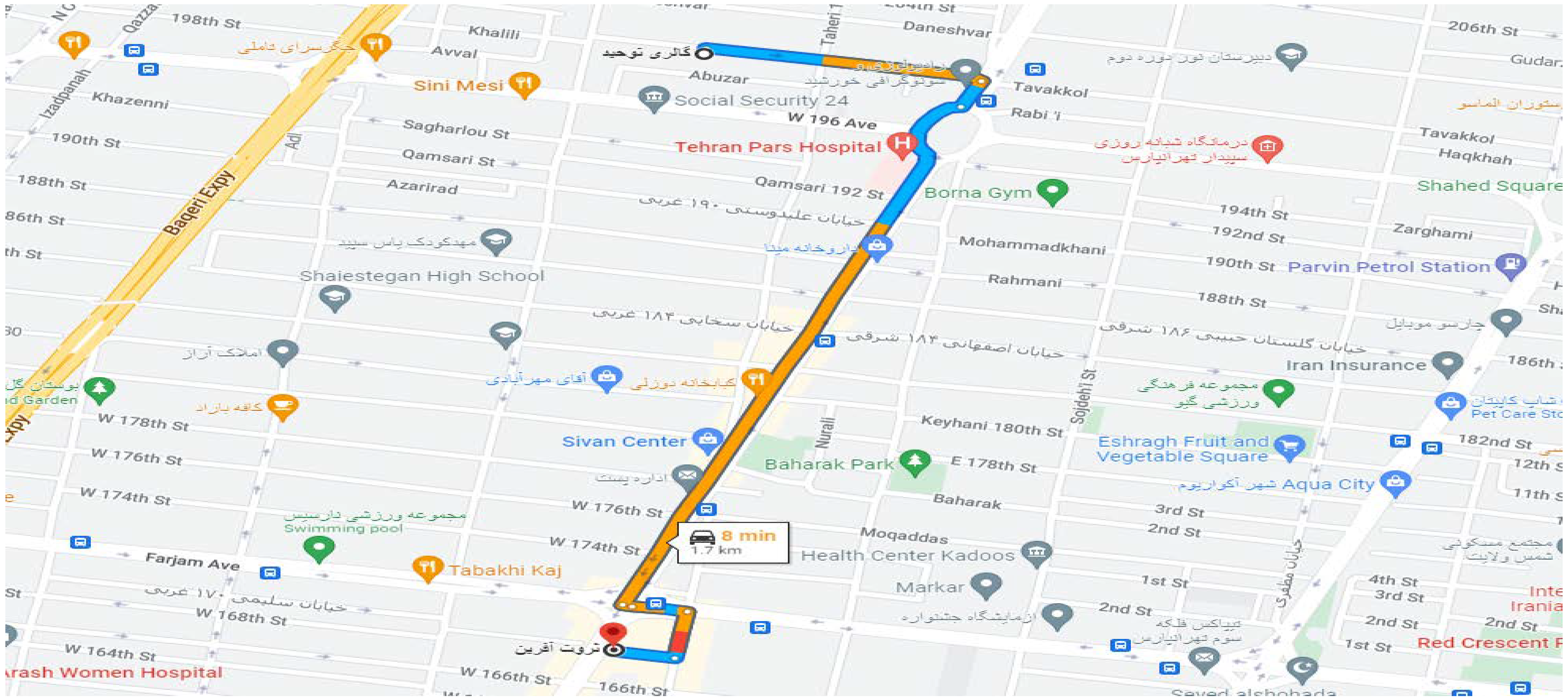
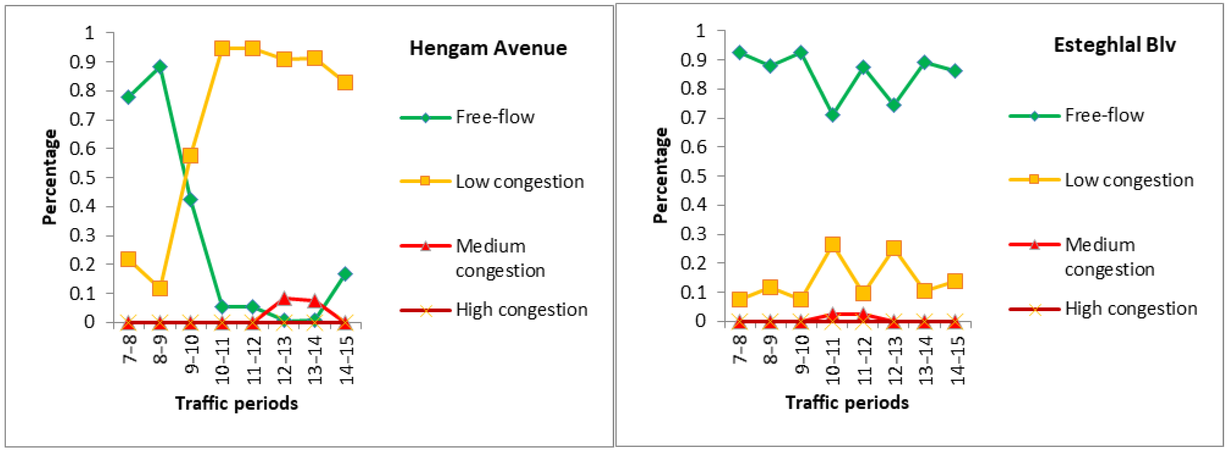
• Congestion highly depends on the road type. The congestion pattern was not similar in different road types. For instance, Figure 5 reveals that the congestion pattern of the route between customer 6 and the depot varied from one section (Esteghlal Boulevard) to another section (Hengam Avenue). On Esteghlal Boulevard, the free-flow traffic mode had the largest share in all periods; however, this amount fluctuated between 70% and 92%. High congestion in both sections was not anticipated during the given traffic period, where in the Hengam Avenue section, free-flow traffic mode had the largest share until 9:00 and then low congestion replaced it until the end of the traffic period (i.e., 15:00).
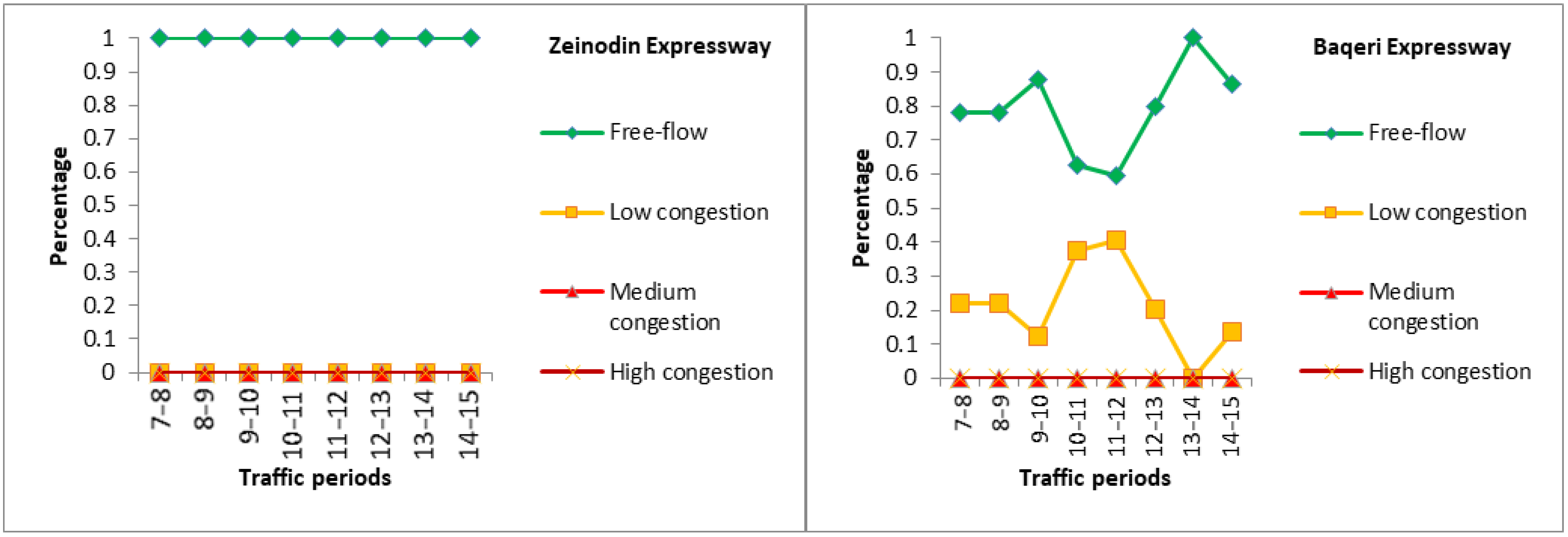
• Congestion patterns in the same road types were different. As an illustration (Figure 6), on Zeinodin Expressway, the pattern was uniform and only a free-flow traffic mode existed during the given traffic period. Nevertheless, both the free-flow mode and low congestion existed on Baqeri Expressway.
• Congestion highly depended on the time. Each section of the route in different traffic modes illustrated different behaviour during the whole period, as follows.

  ○

  Uniform behaviour (i.e., free-flow traffic mode on Zeinodin Expressway)

  ○

  Sinusoidal behaviour (i.e., free-flow traffic mode on Baqeri Expressway)

  ○

  Cosine behaviour (i.e., low congestion on Baqeri Expressway)

  ○

  Ascending behaviour (i.e., low congestion on Hengam Avenue)

  ○

  Descending behaviour (i.e., free-flow traffic mode on Hengam Avenue)

  ○

  Oscillating behaviour (i.e., free-flow traffic mode and low congestion on Esteghlal Boulevard)

Based on the above rules, each section of the route had a different speed profile. It was aessumed that the average speed of the Expressway, Boulevard, Main Street, and Auxiliary Street were equal to 55, 45, 35, and 25 (km/h), respectively. The speed profiles of Zeinodin and Baqeri Expressway of the route between customer 14 and depot were as in Figure 7. As mentioned earlier, there were 6 speed profiles in the literature including increasing, decreasing, V shape, $\Delta$ shape, random, and constant. The speed profile of Baqeri Expressway was constant while for Zeinodin Expressway it was random.

The output of the proposed model was compared with Google Maps’ estimation model and the two models presented in [22,23]. The last two models were selected because their studies were conducted in Iran and the speed profile proposed in them was based on the traffic pattern of this country. Both were designed regardless of intermediate nodes, multiple traffic modes, and dependence of speed profile on a route. Moreover, the above assumptions were not considered for calculating travel time. For validation, 272 routes were analysed and their parameters for this model were computed. In this section, to check the efficiency of the proposed model, a random sample of 30 routes (out of the 272) was presented. The departure time for each of the routes was randomly chosen using MATLAB (version 2012).

Table 4. Travel-time estimation for 30 random samples.

No.	Route	Departure Time		Proposed Model Estimation (min)	Without Intermediate Node, Multiple Traffic Modes, and Route Dependency		Google Estimation (min)
		Hour	Minute
					Alinaghian & Naderipour [23]	Naderipour & Alinaghian [22]
1	1-2	7	33	3.4706	1.95	1.733333	4
2	0-2	13	6	10.1396	7.2	4.430769	10
3	5-1	13	47	5.2694	4.95	3.046154	5
4	1-12	13	51	9.1104	8.4	5.169231	9
5	9-2	11	44	6.4734	2.4	2.181818	7
6	3-4	7	43	8.1017	7.05	6.266667	7
7	3-15	9	5	7.8736	6	5.454545	8
8	7-4	11	6	3.1863	1.92	1.745455	4
9	4-9	14	10	10.1989	7.05	4.338462	10
10	10-5	14	14	13.3933	10.35	6.369231	13
11	9-6	13	6	11.211	8.85	5.446154	11
12	6-11	13	47	8.1976	4.95	3.046154	7
13	8-7	7	57	8.0336	7.8	6.933333	7
14	11-7	13	6	6.277	6.6	4.061538	6
15	12-8	13	47	2.8682	1.8	1.107692	4
16	15-8	13	51	3.7801	2.55	1.569231	4
17	12-9	11	44	10.0803	4.2	3.818182	12
18	11-10	7	43	5.1244	3.3	2.933333	6
19	16-10	9	5	1.454	1.08	0.981818	2
20	14-11	11	6	2.9711	1.56	1.418182	3
21	16-11	14	10	2.7063	1.8	1.107692	3
22	11-16	14	14	3.1024	1.95	1.2	5
23	13-12	8	10	11.2049	9.9	8.8	12
24	16-12	14	16	9.8184	8.7	5.353846	10
25	14-13	14	10	3.2247	2.1	1.292308	5
26	13-14	10	38	2.6125	1.14	1.036364	3
27	13-16	13	0	2.2063	1.2	0.738462	3
28	15-14	8	3	4.4721	3.15	2.8	6
29	16-14	10	9	0.5761	0.264	0.24	1
30	16-15	13	52	9.7121	8.55	5.261538	8

denotes the travel times based on the proposed algorithm logic in Algorithm 2. Google Maps’ estimations, which are based on the date and departure time for each route, were also included.

As a result, the findings of the proposed model were not significantly different from those of Google Maps. Therefore, the authors formulated three hypotheses in which the results of the proposed model, Alinaghian and Naderipour’s model, and Naderipour and Alinaghian’s model, were compared with those of Google Maps based on the dependent-samples t-test. A dependent-sample t-test was run (p < 0.05) using SPSS (version 21) to test these hypotheses (

Table 5. Paired Samples Test between the proposed model and Google Maps.

		Paired Differences					T	Df	Sig. (2-Tailed)
		Mean	Std. Deviation	Std. Error Mean	95% Confidence Interval of the Difference
					Lower	Upper
Pair 1	Google—Proposed	0.271657	0.889936	0.162479	−0.060651	0.603964	1.672	29	0.105

,

Table 6. Paired Samples Test between Alinaghian and Naderipour’s model and Google Maps.

		Paired Differences					T	Df	Sig. (2-Tailed)
		Mean	Std. Deviation	Std. Error Mean	95% Confidence Interval of the Difference
					Lower	Upper
Pair 1	Google—Alinaghian	1.876200	1.668691	0.304660	1.253100	2.499300	6.158	29	0.000

and

Table 7. Paired Samples Test between Naderipour and Alinaghian’s model and Google Maps.

		Paired Differences					t	df	Sig. (2-Tailed)
		Mean	Std. Deviation	Std. Error Mean	95% Confidence Interval of the Difference
					Lower	Upper
Pair 1	Google—Naderipour	3.170617	1.853967	0.338486	2.478334	3.862900	9.367	29	0.000

). Based on the results, due to the significance value (two-tailed) being larger than 0.05 for the first hypothesis, the null hypothesis was not rejected. This meant that there was no significant difference between the estimation of the proposed model and those of Google Maps. Therefore, the proposed model was valid. On the contrary, the p-value for the second and third hypotheses were less than 0.05. Hence, the two model estimations were less than the Google Maps results. Therefore, the null hypothesis was rejected. As a result, these models were examined less accurately.

5. Discussion

Travel-time estimation is a crucial issue in the time-dependent vehicle routing problem. In a green time-dependent vehicle routing optimisation problem, if the travel time is not well estimated, the optimal solution is not obtainable. On the other hand, the values of the objective function (emissions) for different solutions resulted in less accuracy, which leads to incorrect decision making. Therefore, the obtained solution is not capable of minimising the amount of pollution. In this study, attempts were made to develop a model to estimate travel time more accurately. The analysis of Google Maps data in this paper (Section 4) represents a new congestion pattern that has not been addressed in previous research. In this pattern, congestion not only depends on the time but also the route. Therefore, this paper added route dependency as a new concept to the literature. Furthermore, these data denoted that the route between two nodes may have different multiple traffic modes, which should be considered in modeling and have been neglected so far. Due to the dependence of speed on the type of route and the need for route segmentation in real-world modeling, the concept of the intermediate node is introduced in this paper for the first time.

The proposed model assumes that a route has different sections and each section has four traffic modes. Therefore, considering the intermediate node in modeling, which divides a route into different segments, is inevitable. Accordingly, a computational algorithm was developed with different traffic modes (free-flow, low congestion, medium congestion, and high congestion), which were validated against Google Maps. In this context, there was no significant difference between the outputs of this model and those of Google Maps. On the other hand, two other algorithms, Alinaghian and Naderipour [23] and Naderipour and Alinaghian [22], were compared with the above methods in which the intermediate node, multiple traffic modes, and route dependency were not considered. The results showed that these two algorithms cannot estimate travel time like Google Maps and their results are significantly different from Google Maps. Therefore, given that Google Maps’ travel-time estimation model is known as a reference model and is based on reality, the accuracy of the proposed model in this paper is higher than the previously proposed models.

6. Conclusions

In this paper, the authors proposed a new model for estimating travel time in which the intermediate node, route dependency, and multiple traffic modes have been considered. We acknowledge that the closer the estimated travel time is to reality, the better the results and decision-making process. We compared the results of this model with those of Google Maps and two previous models to investigate the effect of the above assumptions on the quality of estimates by statistical analysis. The results showed that using the above assumptions in modeling leads to an increase in the quality of estimations. The main advantage of the proposed model compared to other models is the better representation of reality. However, data collection is difficult to implement in this model. However, if an API service in which the parameters of the proposed model were determined by online navigational and GPS platforms, and applications (e.g., Google Maps, Waze) could be employed, the problems of data gathering and validation would be reduced significantly. Recently, national navigation and GPS in Iran have been developed, called the “Iranian Neshan application—Persian map and router”. This application could also provide all the required information to estimate the parameters of the proposed model. The companies that distribute goods among retailers can use the above algorithm to model and solve the time-dependent vehicle routing problem to schedule the delivery of goods to retailers by their vehicles. Furthermore, through the installation of GPS systems on vehicles and the use of navigation systems, companies can check the driver’s performance each day with the planned route that is obtained from solving the above problem and employ it as an indicator for evaluating the performance of drivers. Companies should implement their developed model based on the above-proposed algorithm for each day. This is because the congestion pattern may be different. Meanwhile, daily customer demand changes and the set of customers to be served on one day may be different from other days.

The most important limitation of the above algorithm is in data collection. In this method, time intervals of one hour are assumed to require less data collection. Considering the average speed for a part of the route in different traffic periods, and the instantaneous change of the speed level from one interval to another interval, are other modelling limitations that exist in other methods as well. The collected data is limited to inner-city routes, only while intercity routes and the combination of intercity routes and routes between two nodes can be considered in solving the model. For future research, developing a new green time-dependent vehicle routing problem with intermediate nodes and multiple traffic modes is applicable. It is also suggested to compare the results of the proposed algorithm with other possible models [34] with the same case study. Ichoua et al [4] developed their model in both static and dynamic modes. The model proposed in this paper is developed based on the static mode. As opposed to the static problem, in the dynamic mode, the number of service requests is not known completely ahead of time; nonetheless, they are rather dynamically revealed as time goes by. Therefore, the authors suggest designing a dynamic version of the proposed model in further investigations by considering intermediate nodes, multiple traffic modes, and route dependency. Intercity routes (i.e., based on the type of route including freeway, highway, etc.) with different speed levels and travel times were considered in the proposed model. Moreover, the proposed model in this article was tested in a case study of a company in the emerging economy of Iran. Although the model has the potential to be universal, larger-scale studies should be carried out and the application of this model to non-city-specific nodes should be explored in the future by other scholars.

References

1. Lin, C.; Choy, K.L.; Ho, G.T.S.; Chung, S.H.; Lam, H.Y. Survey of Green Vehicle Routing Problem: Past and future trends. Expert Syst. Appl. 2014, 41, 1118–1138. [Google Scholar] [CrossRef]
2. Demir, E. Models and Algorithms for the Pollution-Routing Problem and Its Variations. Ph.D. Thesis, University of Southampton, Southampton, UK, 2012. [Google Scholar]
3. Demir, E.; Bektaş, T.; Laporte, G. A review of recent research on green road freight transportation. Eur. J. Oper. Res. 2014, 237, 775–793. [Google Scholar] [CrossRef] [Green Version]
4. Ichoua, S.; Gendreau, M.; Potvin, J.-Y. Vehicle dispatching with time-dependent travel times. Eur. J. Oper. Res. 2003, 144, 379–396. [Google Scholar] [CrossRef] [Green Version]
5. Maden, W.; Eglese, R.W.; Black, D. Vehicle routing and scheduling with time-varying data: A case study. J. Oper. Res. Soc. 2010, 61, 515–522. [Google Scholar] [CrossRef] [Green Version]
6. El-Berishy, N.M.; Scholz-Reiter, B. Development and implementation of a green logistics-oriented framework for batch process industries: Two case studies. Logist. Res. 2016, 9, 9. [Google Scholar] [CrossRef] [Green Version]
7. Goodchild, A. Cost, Emissions, and Customer Service Trade-Off Analysis in Pickup and Delivery Systems; University of Washington: Washington, DC, USA, 2011. [Google Scholar]
8. Pitera, K.; Sandoval, F.; Goodchild, A. Evaluation of Emmissions Reduction in Urban Pickup Systems. Transp. Res. Rec. J. Transp. Res. Board 2011, 2224, 8–16. [Google Scholar] [CrossRef]
9. Alizadeh-Foroutan, R.; Rezaeian, J.; Mahdavi, I. Green vehicle routing and scheduling problem with heterogeneous fleet including reverse logistics in the form of collecting returned goods. Appl. Soft Comput. 2020, 94, 106462. [Google Scholar] [CrossRef]
10. Heni, H.; Coelho, L.C.; Renaud, J. Determining time-dependent minimum cost paths under several objectives. Comput. Oper. Res. 2019, 105, 102–117. [Google Scholar] [CrossRef]
11. Liu, C.; Kou, G.; Zhou, X.; Peng, Y.; Sheng, H.; Alsaadi, F.E. Time-dependent vehicle routing problem with time windows of city logistics with a congestion avoidance approach. Knowl.-Based Syst. 2020, 188, 104813. [Google Scholar] [CrossRef]
12. Pan, B.; Zhang, Z.; Lim, A. Multi-Trip Time-Dependent Vehicle Routing Problem with Time Windows. Eur. J. Oper. Res. 2020, 291, 218–231. [Google Scholar] [CrossRef]
13. Rincon-Garcia, N.; Waterson, B.; Cherrett, T.J.; Salazar-Arrieta, F. A metaheuristic for the time-dependent vehicle routing problem considering driving hours regulations—An application in city logistics. Transp. Res. Part A 2020, 137, 429–446. [Google Scholar] [CrossRef] [Green Version]
14. Sun, P.; Veelenturf, L.P.; Dabia, S.; Woensel, T.V. The Time-Dependent Capacitated Profitable Tour Problem with Time Windows and Precedence Constraints. Eur. J. Oper. Res. 2018, 264, 1058–1073. [Google Scholar] [CrossRef]
15. Tikani, H.; Setak, M. Effi cient solution algorithms for a time-critical reliable transportation problem in multigraph networks with FIFO property. Appl. Soft Comput. 2019, 74, 504–528. [Google Scholar] [CrossRef]
16. Chen, P.W.; Nie, Y.M. Stochastic optimal path problem with relays. Transp. Res. Part C 2015, 59, 48–65. [Google Scholar] [CrossRef]
17. Li, Q.; Nie, Y.M.; Vallamsundar, S.; Lin, J.; Homem-de-Mello, T. Finding Efficient and Environmentally Friendly Paths for Risk-Averse Freight Carriers. Netw. Spat. Econ. 2016, 16, 255–275. [Google Scholar] [CrossRef]
18. Nasri, M.I.; Bekta¸s, T.; Laporte, G. Route and Speed Optimization for Autonomous Trucks. Comput. Oper. Res. 2018, 100, 89–101. [Google Scholar] [CrossRef] [Green Version]
19. Tajik, N.; Tavakkoli-Moghaddam, R.; Vahdani, B.; Mousavi, S.M. A robust optimization approach for pollution routing problem with pickup and delivery under uncertainty. J. Manuf. Syst. 2014, 33, 277–286. [Google Scholar] [CrossRef]
20. Figliozzi, M. The impacts of congestion on time-definitive urban freight distribution networks CO2 emission levels: Results from a case study in Portland, Oregon. Transp. Res. Part C Emerg. Technol. 2011, 19, 766–778. [Google Scholar] [CrossRef]
21. Androutsopoulos, K.N.; Zografos, K.G. An integrated modelling approach for the bicriterion vehicle routing and scheduling problem with environmental considerations. Transp. Res. Part C 2017, 82, 180–209. [Google Scholar] [CrossRef] [Green Version]
22. Naderipour, M.; Alinaghian, M. Measurement, evaluation and minimization of CO2, NOx, and CO emissions in the open time dependent vehicle routing problem. Measurement 2016, 90, 443–452. [Google Scholar] [CrossRef] [Green Version]
23. Alinaghian, M.; Naderipour, M. A novel comprehensive macroscopic model for time-dependent vehicle routing problem with multi-alternative graph to reduce fuel consumption: A case study. Comput. Ind. Eng. 2016, 99, 210–222. [Google Scholar] [CrossRef]
24. Raeesi, R.; Zografos, K.G. The multi-objective Steiner pollution-routing problem on congested urban road networks. Transp. Res. Part B 2019, 22, 457–485. [Google Scholar] [CrossRef] [Green Version]
25. Franceschetti, A.; Honhon, D.; Woensel, T.V.; Bektas, T.; Laporte, G. The time-dependent pollution routing problem. Transp. Res. Part B Methodol. 2013, 56, 265–293. [Google Scholar] [CrossRef] [Green Version]
26. Jabali, O.; Woensel, T.V.; Kok, A.d. Analysis of travel times and CO2 emissions in time-dependent vehicle routing. Prod. Oper. Manag. 2012, 21, 1060–1074. [Google Scholar] [CrossRef]
27. Lu, J.; Chen, Y.; Hao, J.-K.; He, R. The Time-Dependent Electric Vehicle Routing Problem: Model and Solution. Expert Syst. Appl. 2020, 161, 1113593. [Google Scholar] [CrossRef]
28. Çimen, M.; Soysal, M. Time-dependent green vehicle routing problem with stochastic vehicle speeds: An approximate dynamic programming algorithm. Transp. Res. Part D 2017, 54, 82–98. [Google Scholar] [CrossRef]
29. Soysal, M.; Bloemhof-Ruwaard, J.M.; Bektaş, T. The time-dependent two-echelon capacitated vehicle routing problem with environmental considerations. Int. J. Prod. Econ. 2015, 164, 366–378. [Google Scholar] [CrossRef]
30. Soysal, M.; Çimen, M.C. A Simulation Based Restricted Dynamic Programming Approach for the Green Time Dependent Vehicle Routing Problem. Comput. Oper. Res. 2017, 88, 297–305. [Google Scholar] [CrossRef]
31. Fleischmann, B.; Gietz, M.; Gnutzmann, S. Time-Varying Travel Times in Vehicle Routing. Transp. Sci. 2004, 38, 160–173. [Google Scholar] [CrossRef]
32. Mancini, S. A combined multistart random constructive heuristic and set partitioning based formulation for the vehicle routing problem with time dependent travel times. Comput. Oper. Res. 2017, 88, 290–296. [Google Scholar] [CrossRef]
33. Horn, M.E.T. Effcient Modeling of Travel in Networks with Time-Varying Link Speeds. NETWORKS 2000, 36, 80–90. [Google Scholar] [CrossRef]
34. Androutsopoulos, K.N.; Zografos, K.G. A bi-objective time-dependent vehicle routing and scheduling problem for hazardous materials distribution. EURO J. Transp. Logist. 2012, 1, 157–183. [Google Scholar] [CrossRef]
35. Kuo, Y. Using simulated annealing to minimize fuel consumption for the time-dependent vehicle routing problem. Comput. Ind. Eng. 2010, 59, 157–165. [Google Scholar] [CrossRef]
36. Figliozzi, M. Vehicle routing problem for emissions minimization. Transp. Res. Rec. J. Transp. Res. Board 2010, 2197, 1–7. [Google Scholar] [CrossRef] [Green Version]
37. Saberi, M.; Verbas, I.O. Continuous approximation model for the vehicle routing problem for emissions minimization at the strategic level. J. Transp. Eng. 2012, 138, 1368–1376. [Google Scholar] [CrossRef] [Green Version]
38. Xiao, Y.; Konak, A. A simulating annealing algorithm to solve the green vehicle routing & scheduling problem with hierarchical objectives and weighted tardiness. Appl. Soft Comput. 2015, 34, 372–388. [Google Scholar]
39. Zhang, J.; Zhao, Y.; Xue, W.; Li, J. Vehicle routing problem with fuel consumption and carbon emission. Int. J. Prod. Econ. 2015, 170, 234–242. [Google Scholar] [CrossRef]
40. Xiao, Y.; Konak, A. The heterogeneous green vehicle routing and scheduling problem with time-varying traffic congestion. Transp. Res. Part E 2016, 88, 146–166. [Google Scholar] [CrossRef]
41. Huang, Y.; Zhao, L.; Woensel, T.V.; Gross, J.-P. Time-dependent vehicle routing problem with path flexibility. Transp. Res. Part B 2017, 95, 169–195. [Google Scholar] [CrossRef]
42. Saint-Guillain, M.; Paquay, C.; Limbourg, S. Time-Dependent Stochastic Vehicle Routing Problem with Random Requests: Application to online police patrol management in Brussels. Eur. J. Oper. Res. 2020, 292, 869–885. [Google Scholar] [CrossRef]
43. Fan, H.; Zhang, Y.; Tian, P.; Lv, Y.; Fan, H. Time-dependent multi-depot green vehicle routing problem with time windows considering temporal-spatial distance. Comput. Oper. Res. 2021, 129, 105211. [Google Scholar] [CrossRef]
Figure 1. Continuous travel time function.
Sustainability 14 08633 g001
Figure 2. The conceptual framework of intermediate nodes (small circles are intermediate nodes).
Sustainability 14 08633 g002
Figure 3. Warehouse and customer positions.
Sustainability 14 08633 g003
Figure 4. Google Maps’ routing from customer 9 to customer 1.
Sustainability 14 08633 g004
Figure 5. Traffic modes of the different sections of the route between customer 6 and depot.
Sustainability 14 08633 g005
Figure 6. Traffic modes of the expressway sections of the route between customer 14 and depot.
Sustainability 14 08633 g006
Figure 7. Speed profiles of Zeinodin and Baqeri Expressway of the route between customer 14 and depot.
Sustainability 14 08633 g007