Causal Link between Technological Innovation and Inequality Moderated by Public Spending, Manufacturing, Agricultural Employment, and Export Diversification

Abstract

Sustainable Development Goal 10 (SDG10) proposes the reduction of inequalities. This research highlights the importance of considering short- and long-term mechanisms for designing and applying policies to reduce income inequality. Specifically, we test for the causal link between technological innovation and income inequality using a balanced panel data sample from 73 countries worldwide. The inequality–technological innovation relationship is moderated by public spending, manufacturing, employment in agriculture, and export diversification. We use quantile regression techniques to test the impact of technological innovation on income inequality. The results offer robust empirical evidence that in most quantiles, the impact of technological innovation on inequality is positive. This result suggests that the dark side of technological innovation is that it increases income inequality. Furthermore, we find that government spending reduces inequality across all quantiles, while the effect of employment in agriculture and export diversification is inconclusive. Those responsible for social policy towards the achievement of SDG10 must include the advantages of public spending to reduce social disparities and promote social cohesion within countries.

1. Introduction

One of the most worrying social problems of modern economies consists of finding a method to ensure that the benefits of economic progress are distributed equitably to achieve well-being and social cohesion [1]. Income inequality generates economic and social instability that is detrimental to economic progress [2]. The importance of reducing income inequality is reflected in this problem’s inclusion in the agenda of the Sustainable Development Goals (SGD10) of the United Nations. Consequently, income inequality generates concern and academic debates about the agenda of international development organizations and national governments [3]. According to the previous literature, it is possible to classify the mechanisms that determine inequality into two large groups. First, strategies that are based on a short-term time horizon whose actions aim to temporarily mitigate social unrest derived from inequality. Second, there are causal mechanisms that affect inequality in the long run. The mechanisms for reducing income inequality in the short term are mainly conditional cash transfers to low-income families, education and housing programs, and other social policies implemented mainly in developing countries [4,5,6]. Although these policies have a short-term time horizon, the evidence suggests that these efforts can contribute to developing skills and abilities in low-income people in the long run [7,8]. Several recent studies have highlighted the importance and effectiveness of public welfare policies for reducing inequality in the short run [9]. Likewise, the state’s investment in education and infrastructure affects how income is distributed within the economy [10]. In this sense, the social component of public spending can reflect society’s efforts to reduce inequality in the short and long run.

The strategies to gradually reduce inequality in the long term are based on a structural change in the economies and development strategies that involve a significant period [11,12]. One of the main strategies for economic and social progress is the industrialization of countries, particularly in emerging or developing countries [13,14]. Several causal links explain the relationship between inequality and manufacturing in the long run. For example, activities related to manufacturing have increased returns to scale, raised productivity per capita, and promote efficiency [15,16]. In the recent literature on inequality, the evidence linking manufacturing to inequality reduction is limited. Some exceptions are the research studies carried out by Guo et al. [17] and Barua & Ghosh [15]. In this same direction, a second strategy to reduce income inequality in the long term is the sectoral composition of employment. Specifically, countries with a higher share of agricultural employment may be associated with higher levels of inequality. The main argument linking agricultural employment to inequality involves the diminishing returns associated with agriculture. This fact occurs especially in developing countries where agriculture is not very technical; in other words, where monocultures and agriculture for self-consumption predominate [18,19]. Hence, long-term strategies aim to transition the workforce from the agricultural sector to the industrial or service sector [20]. Finally, one of the obstacles developing countries face regarding the mitigation of inequality is having a limited product basket of exports. Therefore, export diversification is necessary as a long-term economic development strategy [21].

In this context, this research aims to examine the link between technological innovation and income inequality using a sample of 73 countries around the world. We include the moderating effect of government spending, manufacturing, agricultural employment, and the export diversification index. We employ modern panel data econometric techniques, namely, quantile regressions and second-generation cointegration techniques. The main justification for using quantile regressions is based on the heterogeneous characteristics of the countries. We expect the slope to have significant differences between the quantiles according to the level of economic progress of each country.

Contrary to expectations, the findings reveal that technological innovation positively correlates with income inequality. This finding suggests the existence of a dark side of technological innovation in terms of social welfare. One possible explanation for this result is that technological innovation produces exclusive benefits for companies, universities, or other institutions that invest in research and development. Those responsible for the social policy must seek mechanisms to promote the distribution of the benefits of innovation in society without limiting the emergence of innovations. The coexistence of the appropriation of the benefits of technology can coexist with income redistribution policies. In addition, we find that public spending is a consistent mechanism for reducing income inequality, which supports the application of policies to promote research and development. Our research contributes to the debate on the dark side of technological innovation. It highlights the importance of public spending, the structure of employment, and the diversification of exports to reduce income inequality.

The rest of the investigation has the following structure. The Section 2 reports the review of the previous literature. The Section 3 describes the main characteristics of the data and the statistical sources. In the Section 4, we present the methodological strategy. The Section 5 presents the results and discusses the findings in conjunction with the previous literature. Finally, the Section 6 contains the conclusions and policy implications of this research.

2. Literature Review

2.1. Technological Innovation-Inequality Nexus

This section reviews the recent literature on the factors that influence income inequality. One causal mechanism that has aroused interest in the academic debate is the inequality–technological innovation nexus. The results are heterogeneous and vary depending on the economies analyzed and the methodology used to obtain the estimators. Although there are differences in the impacts of inequality on the welfare of society between developed and developing countries, there are some common factors that cause it. For example, in OECD countries, changes in innovation rates have significantly impacted wage inequality for workers. In other words, when the rate of innovation increased, the high-tech wage rate also increased relative to the low-tech wage [22]. The learning gap associated with science and technology strengthens the inequality between the groups that benefit from technology and those who do not have access to technology [23]. Fukuhara [24] argues that innovation causes an expansion of inequality in the presence of a prominent industrial sector. However, there is also evidence whose findings indicate that technological progress strengthens economic growth and simultaneously reduces inequality [25]. The benefits of technological progress are better distributed in society through redistribution policies.

Chu et al. [26] and Frydman & Papanikolaou [27] point out that innovation influences greater wage inequality between workers and executives within companies. However, this finding is conditioned by the company’s size or other investment opportunities. In general, the effect of technology may be heterogeneous between productive sectors. It is well known that some sectors generate more linkages than others. For example, a global study of 87 economies found that innovation through the promotion of the internet and mobile diffusion reduces inequality in the short and long term [28]. The insertion of innovation in the health field also contributes to reducing inequality [29].

Similarly, Law et al. [2] highlighted that innovation increased inequality in 23 developed countries due to the moderation of globalization and financial development. In European countries, it was noted that innovation favored agricultural productivity and favored the lowest deciles that are generally engaged in primary sector activities [30]. Innovation increases inequality due to the reduction of workers who are replaced by automatic processes [31]. In an analysis of 46 African countries, the findings indicate that innovation through ICT reduces inequality [32]. It was established in 90 economies from 1970 to 2015 that innovation increased inequality for emerging economies and produced a mixed effect in advanced economies [3]. On the other hand, in a sample of 45 developed and developing countries, the authors concluded that innovation increases income inequality. One of the limitations of the previous literature is that the investigations use predominantly linear methods, omitting the changes in slope along with the distribution.

2.2. Public Spending–Inequality Nexus

The evidence of the relationship between public spending and inequality varies with the development levels of the countries. Glomm & Ravikumar [33] point out that the gap between rich and developing countries widens even though the quality of public education is the same. Therefore, they specified that public education does not reduce inequality in the short term but over the long term. Public spending on education improves the labor force’s skills, facilitating an improvement in income distribution in the long term. For example, the impact of public investment has contributed to further growth in rural areas in China. However, the effect on inequality depends on the type of investment and the region, wherein local management can make a difference in the results achieved [34]. Spending on education must be reinforced with public social spending to achieve the greater effectiveness of social policies. The reduction of public spending on social programs is associated with greater inequality [35]. Government programs for public education and social security are tools to reduce inequality. The level of financing of public spending can cause variations in the impact and the level of development of the countries [36]. However, Rajkumar & Swaroop [37] indicated that public spending does not generate the expected results due to the low levels of governance in poor economies. This fact means that in poorly governed countries, public spending does not influence inequality.

Empirical evidence pointing to an adverse impact of public spending on education on inequality is limited. An exception is the research by Gruber & Kosack [38], who found that public spending on education increases inequality because it is biased towards certain levels of education, which provides disproportionate benefits to the elites. In Norway and the United States, public spending on education accounts for about a third of income inequality and 14% of intergenerational income differences [39]. In Latin America, there was a trend of convergence in the efficiency of public spending from 1970 to 2010. The efficiency lies in the high use of resources towards education for reducing inequality. Countries with higher incomes are the most efficient concerning other economies for their disbursement in this area [40]. Furthermore, public spending in China through public transfers, health care, and pension benefits has closed gender inequality gaps by including women in various social programs [41]. In 76 regions of India, it was detailed that a greater investment in health leads to more private medical care, which in turn leads to greater inequality [42]. The combination of social and health spending in European countries contributes to reducing inequality. Moreover, they reported that social spending decreases inequality in the long term [43]. In OECD countries, it was shown that a 1% increase in social transfers reduced inequality by 0.5%. By including corruption levels in the model, the effect on inequality became heterogeneous across the countries [44]. It was summarized in 18 Latin American countries that there is a positive relationship between public spending and inequality in the short term. However, in the long run, the effect of public spending on inequality disappears [45]. In China, with low public spending on education, income inequalities in old age are accentuated, and a more significant gap is generated between rural and urban areas [46]. These results suggest that public spending on education has a contradictory effect on inequality, indicating that the debate on the link between the two variables is still open.

2.3. Specialization, Export Diversification, and Inequality

There is limited empirical evidence on the link between manufacturing and inequality. The evidence for the United States indicates a threshold effect in the industry–inequality relationship. Initially, the industry increases inequality, decreasing it after the inflection point [47]. The problem of inequality is more evident in industries that are more exposed to international trade. A panel of 27 high- and middle-income countries estimated that the participation of the industrial sector increases inequality. Developing countries are the most affected by inequality when they depend on the manufacturing industry [48]. The industrialization of society is related to greater inequality because of the differences in the productivity of the manufacturing sector compared to the non-manufacturing sector. In a study of China and Europe, the increase in manufacturing was found to promote inequality due to the various skill levels of the population [49].

Analyses of the link between employment in agriculture and inequality are recent. Misra et al. [50] and El Benni & Finger [51] stated that there is a positive link in the variables and that it has been increasing over time. However, the researchers point out that the income obtained from these activities does not reduce inequality within households because they are not stable over time. Additionally, agriculture’s impact on inequality was analyzed in China, where technology was incorporated into production processes. Despite this, the effect of agricultural employment on inequality was found to be relatively small, which was attributed to low-income farmers adapting extremely high-cost technologies [52]. In Indonesia, it was found that workers that are engaged in agricultural activities have higher incomes than non-agricultural households; thus, it was highlighted that agriculture reduces poverty but not inequality in this country [53]. Sutherland [54] stated that there is a positive relationship between these variables and that inequality is reproduced more when there is an inheritance of agricultural land.

Finally, some recent works are grouped in the relationship between export diversification and inequality. Klein et al. [55] have cited that the increase in exports in Germany affects the 30% increase in wage inequalities in manufacturing companies. A study of 116 countries revealed that exports condition economic diversification and lead to a reduction in inequality. The center–periphery structure continues to cause economies’ internal and external inequality [56]. In China, exports increased inequality through the contraction of manufacturing and a higher unemployment rate. The lowest regions were those affected by commercial pressure and the reception of European exports [57]. In 90 economies classified by their income level, a long-run relationship was recently obtained between export diversification and inequality [21]. The regions that export a greater diversity of goods have lower levels of inequality, especially in urban areas. The export structure of countries and their destinations affect inequality [58].

3. Statistical Sources and Data Characteristics

In this research, the dependent variable is income inequality measured by the Gini index. This variable comes from the global base of income inequality, and the values are between zero and one according to the distribution of economic progress benefits among the population’s quantiles. The leading independent variable is technological innovation, which is taken from the World Bank’s development indicators [59] and is the sum of resident and non-resident patents. The manufacturing and employment in agriculture data are from the World Bank Development Indicators and are measured as a percentage of total output and employment, respectively. Finally, we use the export diversification index that was obtained from the International Monetary Fund.

Table 1. Variables and statistical sources.

Variable	Symbol	Description	Measure	Data Source
Inequality	INQ	Measured through the Gini index calculated for each country.	Index.	The World Income Inequality Database.
Innovation	INN	Patent applications are worldwide patent applications filed through the Patent Cooperation Treaty procedure or with a national patent office. In addition, patent applications are worldwide patent applications filed through the Patent Cooperation Treaty procedure or with a national patent office.	Patent applications, nonresidents + Patent applications, residents.	The World Bank
Government spending	GG	Includes all government current expenditures for purchases of goods and services (including compensation of employees). It also includes most expenditures on national defense and security but excludes government military expenditures that are part of government capital formation.	Percentage of GDP.	The World Bank
Manufacturing	MAN	This variable measures the net output of a sector after adding up all outputs and subtracting intermediate inputs. It is calculated without making deductions for the depreciation of fabricated assets or depletion and degradation of natural resources.	Percentage of GDP.	The World Bank
Employment in agriculture	EAG	Employment is defined as persons of working age who were engaged in any activity to produce goods or provide services for pay or profit, whether at work during the reference period or not at work due to temporary absence from a job or the working-time arrangement. The agriculture sector consists of activities in agriculture, hunting, forestry, and fishing.	Percentage of total employment.	The World Bank
Exports diversification	ED	Export diversification can occur across either products or trading partners. Product diversification occurs through introducing new product lines (the extensive margin) or through exporting a more balanced mix of existing products (the intensive margin).	Index.	International Monetary Fund

expands the description of each variable used in the econometric estimates.

Hypothesis 1. 

In the first hypothesis, we propose that technological innovation and income inequality have a negative relationship due to the economic benefits that the emergence of a new patent implies.

Hypothesis 2. 

Our second hypothesis posits a negative relationship between public spending and income inequality. This hypothesis is based on the fact that public social spending immediately impacts the population’s quality of life.

Hypothesis 3. 

The third hypothesis indicates that the manufacturing industry has a negative effect on income inequality. The existence of increasing returns to scale in this sector that benefit workers and entrepreneurs justify this hypothesis.

Hypothesis 4. 

The fourth hypothesis states that a positive relationship exists between the share of agricultural employment and income inequality. The primary justification for this hypothesis is that agriculture has diminishing returns to scale, which harms the workers in this sector.

Hypothesis 5. 

The last hypothesis states that the export diversification index negatively impacts income inequality. The benefits of having a diversified basket of export products support this hypothesis.

Figure 1 illustrates the behavior of the variables during the analysis period. The Figure demonstrates that the largest problem of income inequality is in upper-middle-income countries, where innovation and public spending are relatively low compared to developed countries. In addition, the medium–high income countries are the ones that concentrate the most significant amount of the manufacturing industry and have the most remarkable diversification of exports.

Table 2. Descriptive statistics and correlation matrix.

	Inequality	Innovation	Government Spending	Manufacturing	Employment in Agriculture	Exports Diversification	VIF
Mean	37.56	7.50	16.23	15.53	17.34	2.67
Std. Dev. (Overall)	8.40	2.17	4.92	5.28	16.30	0.97
Std. Dev. (Between)	7.55	2.12	4.68	4.49	15.92	0.92
Std. Dev. (Within)	3.79	0.54	1.60	2.83	3.91	0.35
Min.	13.56	0.70	4.63	0.00	0.03	0.85
Max.	69.96	14.25	28.81	32.45	66.97	6.62
Observations	1825	1825	1825	1825	1825	1825
Countries (N)	73	73	73	73	73	73
Time (T)	25	25	25	25	25	25
Inequality	1.00
	-
Innovation	0.12 *	1.00					1.24
	(0.00)	-
Government spending	−0.34 *	0.07 *	1.00				1.76
	(0.00)	(0.05)	-
Agricultural employment	0.07 *	0.26 *	−0.16 *	1.00			1.59
	(0.04)	(0.00)	(0.00)	-
Manufacturing	0.10 *	−0.24 *	−0.57 *	0.05	1.00		1.21
	(0.00)	(0.00)	(0.00)	(0.53)	-
Exports diversification	0.09 *	−0.35 *	−0.39 *	−0.26 *	0.32 *	1.00	1.48
	(0.00)	(0.00)	(0.00)	(0.00)	(0.00)	-

Note: * Denotes the statistical significance at 5% level.

reports the descriptive statistics, the partial correlation coefficients, and the variance inflator test (VIF) results as a measure of collinearity between the independent variables. Among the aspects of interest, we find no multicollinearity problems between the series, so the estimators obtained are consistent. Likewise, we find that there is greater variability between countries than within them since the SD between is greater than the SD within.

4. Econometric Strategy

The econometric strategy to assess the link between technological innovation and inequality is divided into six stages. In the first stage, a basic panel data regression is estimated using Generalized Least Squares (GLS). This model verifies the effect and direction one variable presents to another. In addition, the model corrects the heteroscedasticity and autocorrelation problems presented by the model to obtain more consistent estimators. This approach is shown in Equation (1). The dependent variable is inequality, and the main independent variable is technological innovation. Other determinants of inequality were also considered, such as public spending, manufacturing, employment in agriculture, and export diversification. Likewise, subscript i and t represent the cross-sectional and temporal information of the study. Finally, the error term symbolized by ${\epsilon }_{it}$ was also added. The econometric strategy is represented in Figure 2.

$$IN{Q}_{it}={\beta }_0+{\beta }_{1}IN{N}_{it}+{\beta }_{2}G{G}_{it}+{\beta }_{3}MA{N}_{it}+{\beta }_{4}EA{G}_{it}+{\beta }_{5}E{D}_{it}+{\epsilon }_{it}$$

(1)

In the second stage, before estimating the econometric models, we apply the cross-section dependence tests. Among them is the Pesaran & Yamagata test [60], which helps to identify the homogeneity of the panel slope. Blomquist & Westerlund [61] emphasized that panel models generally exhibit homogeneity. Therefore, this test poses a null hypothesis: the existence of homogeneity in the data. Additionally, O’Connell [62] points out that the transversal dependence influences the distortion of the results. In this sense, transversal dependence is detected through the Pesaran test [63] that proposed the CD test shown in Equation (2). Chudik & Pesaran [64] emphasized that this test is essential because countries often have socio-economic networks that cause dependency. In this way, the Pesaran [65] and Bailey alongside the Kapetanios and Pesaran [66] tests are used to establish more consistent estimates.

$$CD=\left[\frac{2T}{N\left(N-1\right)}\left({\displaystyle \sum }_{i=1}^{N-1}{\displaystyle \sum }_{j=i+1}^N\widehat{p}ij\right)\right]$$

(2)

In the third stage, the quantile regressions developed by Koenker & Bassett [67] are estimated. This methodology facilitates the analysis of the effect of the explanatory variables on inequality under a conditioned quantile. Two estimators were used: the Powell model [68] and Chernozhukov et al.’s method [69]. Powell’s model [68] includes a generalized quantile implementor relative to Powell’s estimator [70]. Instead, Chernozhukov et al. [69] incorporated the bootstrap method to accelerate the acquirement of more robust results. Equation (3) presents the respective formal approach.

$$Q_i=Q_i|X_{\mathit{it}}=\left({\alpha }_0+{\beta }_0\right)+{\beta }_1{\left(X_1\right)}_{it}+{\beta }_2{\left(X_2\right)}_{it}+\dots {\beta }_n{\left(X_3\right)}_{it}+{\epsilon }_{it}$$

(3)

In Equation (3), Q_i identifies the analyzed quantile corresponding to each decile. The intercept of the quantile regression is represented by the term (${\alpha }_0+{\beta }_0$). The coefficients ${\beta }_1,{\beta }_2, {\beta }_n$ reflect the impact of the variables $X_1,X_2, X_n$ in each quantile on inequality. When the transversal dependence in the panel is verified, the second-generation unit root tests are applied. That is why, in the fourth stage, the Breitung [71], Pesaran [63], and Herwartz and Siedenburg [72] tests were used. These tests allow for the discarding of the trend behavior of the variables to continue with the cointegration analysis. The Westerlund second-generation cointegration test [73] suggested by Persyn and Westerlund [74] is also applied. This methodology considers the existence of transversal dependence and heterogeneity within the panel. Likewise, it uses four statistics that determine the group’s cointegration and the complete panel. Its expression is shown below:

$$Y_{i,t}={\delta }_i{d}_t+{\alpha }_i\left(y_{i,t-1}-{\beta }_i{X}_{i,t-1}\right)+{\displaystyle \sum }_{j=1}^{Pi}{\alpha }_{ij{Y}_{it-j}}+{\displaystyle \sum }_{j=-qi}^{pi}{y}_{ij}{X}_{it-j}+{\epsilon }_{i,t}$$

(4)

where $d_t$ reveals the deterministic component of the model. This component can adopt values of $d_t=0$, $d_t=1,$ and $d_t=1-t$, which indicate the presence or absence of a constant in the dependent variable. The terms pi and qi represent the delay or advance orders of the transverse units. In the fifth stage, the short- and long-term elasticity is estimated. In the short term, the augmented mean group estimator (AMG) developed by Eberhardt and Bond [75] and Eberhardt and Teal [76] and the common correlated effects mean group estimator (CCE-MG) proposed by Pesaran [77] and modified by Kapetanios et al. [78] are used. The two models also include the cross-sectional dependence and heterogeneity of the parameters through a common dynamic factor. Equation (5) details the expression of the AMG estimator. In this equation, β_i corresponds to the coefficients obtained, which are represented in Equation (6):

$$AMG=N^{-1}{\displaystyle \sum }_{i=1}^N{\beta }_i$$

(5)

$$Y_{it}={\alpha }_i+B_i\Delta x_{it}+{\phi }_i{f}_t+{\displaystyle \sum }_{t=2}^T{X}_t+{\epsilon }_{it}$$

(6)

The CCE-MG estimator is presented in Equation (7). The aforementioned estimator, in addition to the traditional expressions, includes the average value of the dependent variable and the regressor variables denoted by $\overline{y}$ and $\overline{x}$ in Equation (8). The common dynamic factor is identified by $f_t$ in both estimators.

$$CCE-MG=N^{-1}{\displaystyle \sum }_{i=1}^N{\beta }_i$$

(7)

$$Y_{it}={\alpha }_i+B_i{x}_{it}+{\theta }_i{\overline{y}}_{it}+{\delta }_i{\overline{x}}_{it}+{\phi }_i{f}_t+{\epsilon }_{it}$$

(8)

To determine the long-term elasticities, Fully Modified Ordinary Least Squares (FMOLS) and Ordinary Least Squares (DOLS) were used. Finally, in the sixth stage, the causality is established for each pair of model variables through the Dumitrescu and Hurlin test [79] explained in Equation (9).

$$Y_{it}={\alpha }_i+{\displaystyle \sum }_{K=1}^K{\gamma }_i^k{Y}_{it-K}+{\displaystyle \sum }_{K=1}^K{\beta }_i^k{X}_{it-k}+{\epsilon }_{it}$$

(9)

In the causality model, $Y_{it}$ is the inequality corresponding to the dependent variable. The terms ${\gamma }_i^k$ and ${\beta }_i^k$ tend to fluctuate in the countries of analysis. Likewise, $X_{it}$ encompasses the explanatory variables. The null hypothesis of this test consists of the absence of a causal relationship in the transversal units of the panel.

5. Results and Discussion

Table 3. Results of generalized least squared-GLS regressions.

	GLOBAL	HIC	MHIC	MLIC
Innovation	0.34 ***	0.34 ***	0.20	−0.33
	(8.08)	(8.08)	(0.80)	(−1.67)
Government spending	−0.83 ***	−0.83 ***	−0.14	−0.30 ***
	(−29.18)	(−29.18)	(−1.59)	(−4.09)
Manufacturing	−0.01	−0.01	−0.02	0.21 **
	(−0.64)	(−0.64)	(−0.43)	(3.16)
Employment in agriculture	−0.08 ***	−0.08 ***	−0.12 *	−0.09 ***
	(−8.57)	(−8.57)	(−2.47)	(−5.03)
Export diversification index	0.06	0.06	−0.35	−1.11 **
	(0.50)	(0.50)	(−1.00)	(−2.66)
Constant	49.65 ***	49.65 ***	47.98 ***	46.69 ***
	(48.05)	(48.05)	(15.93)	(12.58)
Observations	1825	1825	550	400
Hausman test (p-value)	0.00	0.00	0.03	0.01
Autocorrelation test (p-value)	0.86	0.76	0.89	0.88
Fixed effects (time)	No	No	No	No
Fixed effects (country)	No	No	No	No
Countries (N)	73	73	22	16
Chi-squared	1306.9	1306.9	9.61	95.01

Note: t statistics in parentheses * p < 0.05, ** p < 0.01, *** p < 0.001.

reports the results of a basic GLS model to determine the effect of covariates on inequality. We find that innovation positively affects inequality globally and in HICs. One possible explanation for this result is that when innovative activity increases through a greater number of patents, only high-income people gain access, resulting in greater inequality. In addition, as the HICs are the countries with the greatest technological development, the impact is more evident in this group because innovation translates into greater diversification of the products and services. Public spending generates an opposite effect; that is, it significantly reduces inequality in all groups of countries, except for the MHIC, where there is no statistical significance. When countries allocate more public spending on health and education, the opportunities of the population are improved, and it is possible to reduce income inequality. Likewise, social programs contribute to raising living standards. The result of the innovation is contradictory to research such as that of Ojha et al. [25], Drummond-Lage et al. [29], and Adams and Akobeng [32], who contended that this variable reduces inequality by applying technology in various fields of the economy. However, it agrees with Butler and Dueker [22] and Gravina and Lanzafame [3], who argued that automation in production systems increases inequality due to the unemployment of unskilled workers.

For public spending, Glomm and Kaganovich [36], Shen et al. [41], and d’Agostino et al. [44] highlighted that transfer programs, public education, social security, and health are the central mechanisms for reducing inequality. Even so, due to the low levels of governance in developing countries, more significant results are not obtained [37]. The effect of manufacturing on inequality only shows significance in the MLICs. This finding is supported by the automation of production processes that generate unemployment in the populations with limited academic education. Employment in agriculture decreases inequality in all groups of countries, with values that fluctuate between 0.08 and 0.12 points. This fact occurs because most people with medium and low incomes work in this type of activity. As there is a high consumption of food products, a greater demand for personnel is promoted, providing income to this sector. Finally, export diversification significantly reduces inequality only for MLICs. This variable allows countries to be more competitive in the international trade environment. This result is even more interesting in developing countries that depend on the rent of natural resources, which causes stagnation in their economies. On employment in agriculture, the result disagrees with Mishra et al. [50] and El Benni and Finger [51] since these authors reported that the income obtained in these activities is not stable over time. In the diversification of exports, the expected result was obtained, but emphasis must be placed on the commercial structure of the countries [58].

Panel data models generally present heterogeneity in a slope; its presence was verified through the test developed by Pesaran and Yamagata [60].

Table 4. Test for slope homogeneity of Pesaran and Yamagata (2008).

Tests	Delta	p-Value
∆	29.16 ***	0.00
∆adj	34.37 ***	0.00

Note: t statistics in parentheses, and *** p < 0.01.

shows the results that allow for the rejection of the null hypothesis with a significance level of 1%. Furthermore, it is verified that the slope coefficients are not equal, which contributes to the acquirement of consistent estimators.

We highlight the existence of transversal dependency in the variables. To this end, the Pesaran [65] and Bailey et al. [66] tests presented in

Table 5. Cross-section dependence test.

Variables	Pesaran (2014) [65]		Bailey et al. (2015) [66]
	Statistic	p-Value	Statistic	p-Value
Inequality	3.12 ***	0.00	253.58 ***	0.00
Innovation	9.21 ***	0.00	253.70 **	0.01
Government spending	22.18 ***	0.00	253.39 ***	0.00
Manufacturing	84.26 ***	0.00	250.48 ***	0.00
Employment in agriculture	215.05 ***	0.00	252.36 ***	0.00
Exports diversification	27.60 ***	0.00	253.56 ***	0.00

Note: t statistics in parentheses ** p < 0.01, *** p < 0.001.

were used. In both tests, the null hypothesis of the independence of the cross-sections for all variables was rejected. The results indicate that there is a dependence on the cross-sections, which in turn affects the unit root tests used before the cointegration phase. The dependency in the cross-sections implies that the analyzed countries depend on each other due to commercial or political aspects.

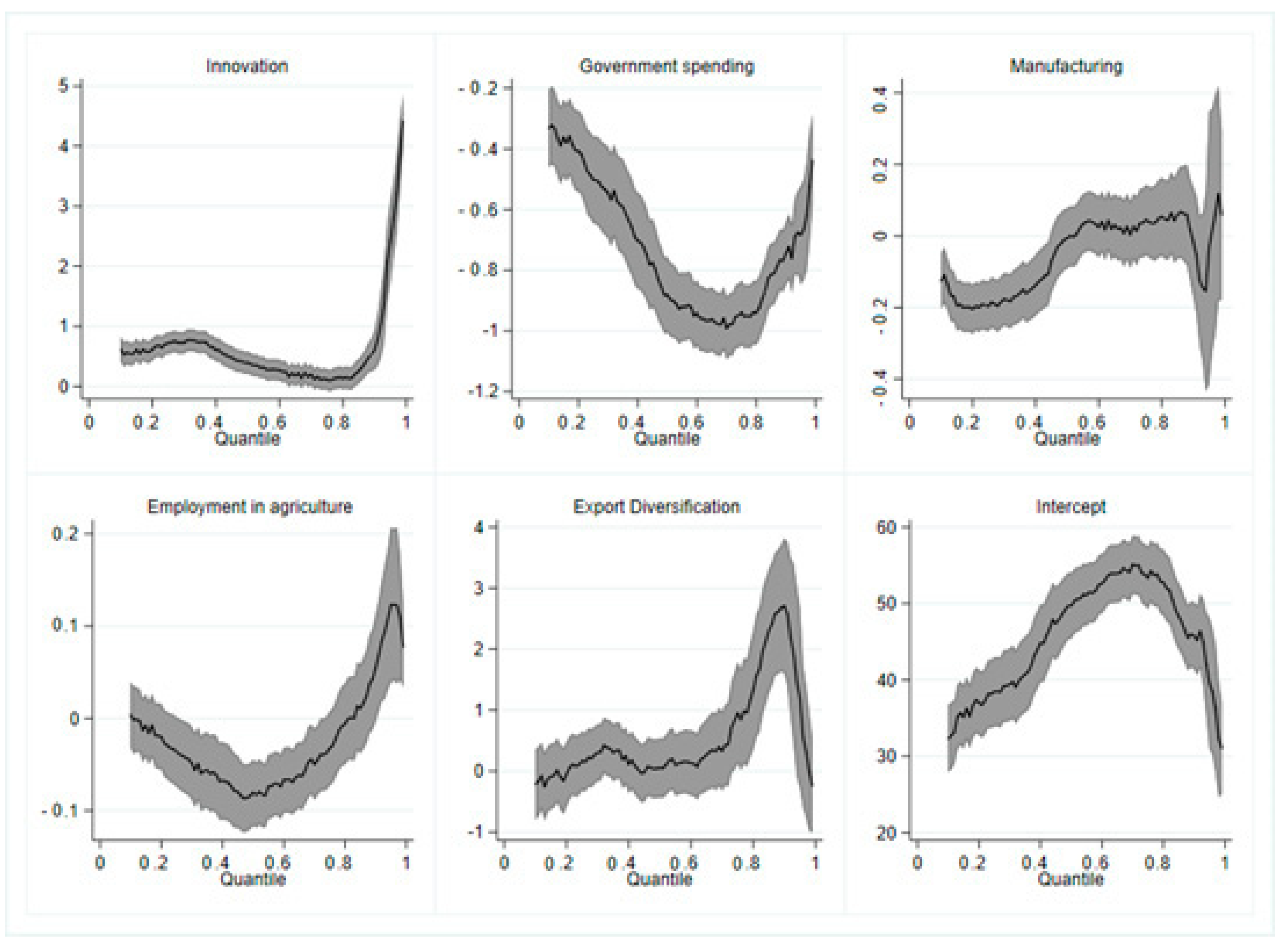
Figure 3 shows the graph of quantiles for each variable of the model to verify its heterogeneous behavior concerning a normal distribution. It is evident that all the variables shown are not linear. This outline is most noticeable in public spending, employment in agriculture, and export diversification. Likewise, most variables maintain a similar pattern within the distribution. In particular, at the beginning and the end, they present a positive effect; that is to say, the points are on the reference line. Although in the end, they tend to point to a negative trend. However, the points on the far right of public spending are located below the line. In other words, innovation, manufacturing, employment in agriculture, and export diversification increase inequality in the first and last quantiles. On the contrary, in the low quantiles of public spending, public spending increases inequality, and in the high quantiles, public spending decreases income inequality.

The results of the Powell [68] quantile regressions obtained through fixed effects are reported in

Table 6. Powell (2016) fixed effect estimators’ model.

	0.1	0.2	0.3	0.4	0.5	0.6	0.7	0.8	0.9
73 countries
Innovation	0.60 ***	0.51 ***	0.77 ***	0.56 *	0.31	0.19	0.36	0.14	0.70 ***
	(18.13)	(4.11)	(5.53)	(2.52)	(1.69)	(1.45)	(1.81)	(1.67)	(6.23)
Government spending	−0.35 ***	−0.52 ***	−0.51 ***	−0.74 ***	−0.95 ***	−1.01 ***	−0.83 ***	−0.94 ***	−0.76 ***
	(−11.28)	(−3.34)	(−5.08)	(−4.61)	(−6.55)	(−10.82)	(−6.12)	(−7.65)	(−17.76)
Manufacturing	−0.12 ***	−0.23 ***	−0.18 ***	−0.14 **	−0.05	0.01	0.12	0.04	−0.07
	(−13.04)	(−5.20)	(−6.90)	(−3.10)	(−0.70)	(0.12)	(1.27)	(0.60)	(−1.05)
Employment in agriculture	0.001	−0.04	−0.04 *	−0.08 *	−0.10 ***	−0.07 ***	−0.03	−0.01	0.06 ***
	(0.10)	(−1.52)	(−2.34)	(−2.30)	(−3.33)	(−5.57)	(−1.90)	(−0.77)	(6.03)
Export diversification	−0.374	−0.43	0.33	0.09	−0.19	−0.15	1.18	1.25	2.22 ***
	(−1.71)	(−0.85)	(0.99)	(0.19)	(−0.40)	(−0.34)	(1.58)	(1.93)	(6.38)
Constant	33.15 ***	41.44 ***	38.33 ***	45.95 ***	53.05 ***	55.46 ***	47.17 ***	53.39 ***	47.48 ***
	(23.95)	(7.06)	(9.27)	(6.76)	(8.24)	(12.31)	(6.59)	(10.35)	(14.16)
Observations	1825	1825	1825	1825	1825	1825	1825	1825	1825
High Income Countries
Innovation	0.68 ***	0.60 ***	0.62 ***	0.69 **	0.51	0.64 ***	0.74	0.43 ***	0.57 ***
	(9.38)	(18.13)	(3.52)	(3.09)	(1.67)	(3.31)	(1.78)	(4.03)	(7.22)
Government spending	−0.49 ***	−0.35 ***	−0.46 **	−0.50 **	−0.78 ***	−0.77 ***	−0.80 ***	−0.95 ***	−0.78 ***
	(−10.66)	(−11.28)	(−3.13)	(−3.25)	(−3.60)	(−8.11)	(−3.55)	(−10.23)	(−17.07)
Manufacturing	−0.42 ***	−0.12 ***	−0.45 ***	−0.46 ***	−0.51 ***	−0.43 ***	−0.34 ***	−0.36 ***	−0.26 ***
	(−15.85)	(−13.04)	(−8.77)	(−7.48)	(−5.54)	(−6.91)	(−3.64)	(−8.48)	(−12.81)
Employment in agriculture	0.26 ***	0.001	0.20 ***	0.20 ***	0.16	0.23 ***	0.25 *	0.18 ***	0.38 ***
	(9.79)	(0.10)	(4.21)	(4.16)	(1.68)	(4.25)	(2.19)	(3.57)	(9.05)
Export Diversification	0.11	−0.37	−0.33	−0.14	−0.58	0.20	2.80	2.52 ***	5.34 ***
	(0.37)	(−1.71)	(−0.44)	(−0.18)	(−0.78)	(0.35)	(1.60)	(4.09)	(17.71)
Constant	37.54 ***	33.15 ***	42.04 ***	43.01 ***	52.90 ***	49.47 ***	43.69 **	51.47 ***	40.60 ***
	(14.74)	(23.95)	(6.24)	(5.69)	(5.22)	(8.69)	(3.27)	(11.10)	(16.47)
Observations	875	1825	875	875	875	875	875	875	875
Middle-High Income Countries
Innovation	1.37 ***	0.90 ***	0.82 ***	0.63 ***	0.23	−0.05	−0.35 **	−0.32	−0.90 ***
	(16.22)	(3.41)	(3.35)	(3.79)	(1.26)	(−0.24)	(−2.66)	(−0.95)	(−5.25)
Government spending	−1.16 ***	−1.33 ***	−1.22 ***	−1.03 ***	−1.08 ***	−0.65 **	−0.21	0.42	0.51 ***
	(−15.13)	(−7.55)	(−9.65)	(−6.66)	(−6.95)	(−2.93)	(−0.71)	(1.46)	(6.62)
Manufacturing	−0.04	0.08 **	0.06	0.08	−0.02	−0.09	−0.25	−0.11	−0.20 ***
	(−1.60)	(3.17)	(1.80)	(1.31)	(−0.27)	(−0.66)	(−1.72)	(−0.50)	(−3.31)
Employment in agriculture	−0.30 ***	−0.27 ***	−0.23 ***	−0.21 ***	−0.24 ***	−0.24 ***	−0.26 ***	−0.18 ***	−0.24 ***
	(−30.39)	(−24.52)	(−15.04)	(−14.06)	(−6.89)	(−5.82)	(−8.14)	(−3.96)	(−18.64)
Export diversification	−3.81 ***	−2.97 ***	−1.93 ***	−1.39 **	−2.35 **	−2.65 *	−3.59 ***	−2.84 **	−3.78 ***
	(−18.11)	(−5.59)	(−4.95)	(−2.91)	(−3.13)	(−2.26)	(−3.56)	(−3.21)	(−21.30)
Constant	57.84 ***	61.90 ***	59.24 ***	57.44 ***	68.20 ***	68.87 ***	74.52 ***	61.69 ***	73.14 ***
	(26.70)	(9.78)	(11.48)	(10.34)	(9.56)	(6.73)	(7.00)	(4.65)	(19.83)
Observations	550	550	550	550	550	550	550	550	550
Middle-Low Income Countries
Innovation	0.22 ***	0.34	0.36	−1.58	−0.80	−1.60 *	−3.26 **	−2.19 ***	−2.45 ***
	(5.99)	(1.47)	(1.65)	(−1.39)	(−1.05)	(−2.07)	(−2.81)	(−4.36)	(−17.25)
Government spending	−0.55 ***	−0.25	−0.07	−0.78	−0.32	−0.50 *	−1.20 *	−0.68 ***	−0.59 ***
	(−12.28)	(−1.87)	(−0.62)	(−1.78)	(−1.54)	(−2.04)	(−2.56)	(−3.81)	(−15.85)
Manufacturing	−0.12 ***	0.09	0.22 ***	−0.15	0.17	0.14	−0.27	0.35 *	0.72 ***
	(−4.51)	(1.66)	(4.65)	(−0.51)	(1.41)	(1.23)	(−0.57)	(2.26)	(18.42)
Employment in agriculture	−0.04 ***	0.02	−0.02	−0.15 **	−0.09 ***	−0.06 *	−0.15	−0.07 *	−0.07 **
	(−6.84)	(0.98)	(−0.77)	(−3.30)	(−4.39)	(−2.12)	(−1.96)	(−2.03)	(−2.89)
Export Diversification	1.31 ***	1.02	0.64	−4.09	−1.91	−3.70 *	−8.05 *	−4.60 ***	−4.16 ***
	(10.47)	(1.42)	(1.33)	(−1.53)	(−1.20)	(−2.54)	(−2.42)	(−3.52)	(−13.14)
Constant	33.65 ***	26.38 ***	27.24 ***	76.17 **	52.65 ***	66.77 ***	111.3 ***	77.15 ***	73.90 ***
	(20.65)	(4.03)	(5.15)	(2.82)	(3.57)	(4.47)	(3.33)	(5.99)	(27.27)
Observations	400	400	400	400	400	400	400	400	400

Note: t statistics in parentheses * p < 0.05, ** p < 0.01, *** p < 0.001.

. The heterogeneity in the parameters is one of the structural characteristics of the results. Innovation generates a positive effect on inequality in most quantiles for HICs. At the other levels of development, inequality increases in the first four quantiles and decreases in the last. On the other hand, public spending decreases inequality for all quantiles at the global level and in the HICs. Unlike the MHIC, inequality is significantly reduced up to quantile six and increases in quantile nine. In the MLIC, the effect is negative in quantile one and from six to nine. In contrast, manufacturing reduces inequality throughout the distribution in the HIC, and there are heterogeneous effects in the rest of the groups. Globally, inequality falls to the fourth quantile. In the MHIC, the impact is positive for the second quantile and negative for the ninth. In the MLIC, inequality is reduced in quantile one and increases in the eighth and ninth quantiles.

Employment in agriculture increases inequality for all quantiles in the HICs and decreases it in the MHICs and MLICs. However, the negative effect is concentrated in the middle quantiles at around 0.10 points at a global level. Export diversification reduces inequality across all quantiles in the MHICs. In the MLICs, the impact is negative only in the last quantiles, while at the global level and in HICs, inequality increases in the eighth and ninth quantiles. The heterogeneous effects of these variables on inequality are evident at the global level and each income level. Innovation increases inequality in the first quantiles because there are learning gaps among the population [23]. Furthermore, Chu et al. [26] and Frydman and Papanikolaou [27] reported that innovation gives way to differences between workers who correspond to the low or middle deciles and executives who are part of the high deciles. It disagrees with Madsen and Strulik [30], who reported that inequality decreased in the first deciles due to innovation adjusted to the primary sector.

Public spending significantly reduces inequality in most quantiles. Gruber and Kosack [38] proposed that public spending is aimed at promoting tertiary education that mainly benefits the elites. The highest deciles generally choose to access private services creating greater inequality within countries [42]. As for manufacturing, the negative impact on inequality is obtained by favoring the lowest deciles. Chen [80] justifies this synergy by the participation of low-skilled labor in industrial activities that allow them to provide income to this population group. After all, the relative changes in wages respond to changes in each worker’s labor productivity, the countries’ institutional arrangements, and the demand for a qualified labor force [81,82,83]. However, Borrs and Knauth [49] maintain the idea that the different levels of qualification can create greater inequality. The highest quantiles have more technical skills than the lowest quantiles, which is where the disparities are generated. Given this relationship, Klein et al. [55] revealed that export diversification reduces inequality and increases it by causing wage inequality for export goods.

Table 7. Results of Chernozhukov et al. (2020) quantile regression.

	0.1	0.2	0.3	0.4	0.5	0.6	0.7	0.8	0.9
73 countries
Innovation	0.57 ***	0.73 ***	0.65 ***	0.39 ***	0.28 **	0.16	0.15	0.53 ***	4.42 ***
	(6.08)	(7.90)	(6.67)	(4.16)	(3.08)	(1.78)	(1.64)	(3.78)	(19.59)
Government spending	−0.41 ***	−0.53 ***	−0.69 ***	−0.88 ***	−0.95 ***	−0.96 ***	−0.94 ***	−0.77 ***	−0.44 ***
	(−6.00)	(−7.00)	(−8.52)	(−13.64)	(−17.17)	(−18.12)	(−17.58)	(−14.84)	(−5.71)
Manufacturing	−0.20 ***	−0.19 ***	−0.15 ***	−0.01	0.03	0.03	0.05	0.02	0.06
	(−5.67)	(−4.98)	(−3.40)	(−0.24)	(0.78)	(0.55)	(0.89)	(0.24)	(0.49)
Employment in agriculture	−0.02	−0.04 *	−0.07 **	−0.08 ***	−0.07 ***	−0.04 *	−0.01	0.04	0.08 ***
	(−1.06)	(−2.23)	(−3.21)	(−4.61)	(−4.17)	(−2.32)	(−0.38)	(1.54)	(3.46)
Export diversification	−0.16	0.26	0.25	0.04	0.15	0.40	1.15 *	2.68 ***	−0.24
	(−0.59)	(1.09)	(1.04)	(0.17)	(0.55)	(1.22)	(2.43)	(5.04)	(−0.61)
Constant	37.37 ***	39.24 ***	43.91 ***	49.70 ***	52.48 ***	54.09 ***	52.90 ***	46.00 ***	31.07 ***
	(17.07)	(16.35)	(16.96)	(22.38)	(26.52)	(27.77)	(24.45)	(21.02)	(10.08)
Observations	1825	1825	1825	1825	1825	1825	1825	1825	1825
High income countries
Innovation	0.68 ***	0.70 ***	0.73 ***	0.74 ***	0.67 ***	0.45 ***	0.47 ***	0.48 ***	0.62 ***
	(6.40)	(7.28)	(7.41)	(6.50)	(5.29)	(3.65)	(4.41)	(4.35)	(9.58)
Government spending	−0.47 ***	−0.36 ***	−0.44 ***	−0.57 ***	−0.72 ***	−0.92 ***	−0.88 ***	−0.79 ***	−0.66 ***
	(−8.46)	(−6.56)	(−6.76)	(−7.11)	(−8.25)	(−13.64)	(−13.80)	(−13.86)	(−21.02)
Manufacturing	−0.42 ***	−0.43 ***	−0.45 ***	−0.46 ***	−0.42 ***	−0.37 ***	−0.38 ***	−0.22 **	−0.24 ***
	(−10.60)	(−11.47)	(−11.70)	(−10.04)	(−7.84)	(−6.28)	(−6.26)	(−2.80)	(−5.47)
Employment in agriculture	0.21 ***	0.28 ***	0.20 ***	0.23 ***	0.25 ***	0.22 **	0.19 **	0.29 ***	0.62 ***
	(4.60)	(5.65)	(4.51)	(4.66)	(4.36)	(3.21)	(3.07)	(3.80)	(11.61)
Export diversification	−0.15	0.06	−0.05	−0.06	0.08	1.59 *	2.73 ***	5.06 ***	6.99 ***
	(−0.57)	(0.19)	(−0.15)	(−0.16)	(0.19)	(2.18)	(3.38)	(5.86)	(15.20)
Constant	39.53 ***	37.92 ***	40.95 ***	44.54 ***	48.02 ***	51.51 ***	49.51 ***	41.46 ***	35.25 ***
	(24.00)	(20.58)	(17.55)	(14.91)	(14.85)	(16.54)	(16.32)	(14.35)	(22.30)
Observations	875	875	875	875	875	875	875	875	875
Middle-high income countries
Innovation	0.88 ***	0.77 ***	0.56 **	0.36	0.28	0.07	−0.33	−0.79 *	−1.66 ***
	(4.19)	(3.77)	(2.93)	(1.66)	(1.06)	(0.19)	(−0.86)	(−1.98)	(−8.39)
Government spending	−1.23 ***	−1.27 ***	−1.19 ***	−0.98 ***	−0.60 *	0.14	0.16	0.34	0.93 ***
	(−10.31)	(−10.70)	(−9.50)	(−5.63)	(−2.35)	(0.52)	(0.71)	(1.72)	(8.66)
Manufacturing	0.01	0.01	0.01	0.04	−0.002	−0.08	−0.24	−0.24	−0.28 ***
	(0.23)	(0.12)	(0.14)	(0.51)	(−0.02)	(−0.58)	(−1.59)	(−1.56)	(−4.00)
Employment in agriculture	−0.30 ***	−0.25 ***	−0.21 ***	−0.23 ***	−0.21 ***	−0.19 ***	−0.20 ***	−0.22 ***	−0.25 ***
	(−9.62)	(−7.01)	(−5.61)	(−5.63)	(−4.77)	(−3.59)	(−3.45)	(−3.84)	(−9.09)
Export diversification	−3.29 ***	−2.12 ***	−1.78 ***	−1.87 ***	−1.72 **	−2.25 ***	−3.17 ***	−3.78 ***	−3.25 ***
	(−8.12)	(−5.05)	(−4.13)	(−3.73)	(−3.12)	(−3.80)	(−5.45)	(−6.52)	(−9.52)
Constant	63.90 ***	62.19 ***	62.59 ***	63.07 ***	59.95 ***	57.62 ***	68.17 ***	74.69 ***	78.19 ***
	(22.05)	(22.15)	(22.52)	(19.08)	(15.90)	(11.67)	(13.65)	(14.02)	(29.72)
Observations	550	550	550	550	550	550	550	550	550
Middle-low income countries
Innovation	0.20	0.42	−0.21	−0.82	−0.87	−1.54 **	−1.54 **	−2.24 ***	−1.21
	(0.57)	(1.09)	(−0.45)	(−1.45)	(−1.63)	(−3.08)	(−3.24)	(−4.69)	(−0.70)
Government spending	−0.38	−0.05	−0.23	−0.33	−0.31 *	−0.50 ***	−0.54 ***	−0.52 ***	−0.05
	(−1.80)	(−0.31)	(−1.37)	(−1.88)	(−2.02)	(−3.81)	(−4.66)	(−4.27)	(−0.27)
Manufacturing	0.02	0.20	0.29 *	0.15	0.18	0.40 **	0.45 **	0.79 ***	1.18 ***
	(0.16)	(1.63)	(2.20)	(1.15)	(1.39)	(2.65)	(2.94)	(4.07)	(5.31)
Employment in agriculture	0.05	0.005	−0.06	−0.20 *	−0.04	−0.05	−0.03	−0.03	−0.26 *
	(0.85)	(0.09)	(−1.50)	(−2.55)	(−1.06)	(−1.37)	(−0.70)	(−0.44)	(−2.15)
Export diversification	1.12	1.83 *	−0.75	−1.85	−2.51 *	−2.92 ***	−3.32 ***	−3.41 ***	−5.44 ***
	(1.26)	(1.97)	(−0.71)	(−1.60)	(−2.42)	(−3.42)	(−4.51)	(−4.68)	(−9.64)
Constant	29.44 ***	22.81 **	39.84 ***	52.73 ***	53.78 ***	61.35 ***	63.56 ***	66.53 ***	72.03 ***
	(3.34)	(2.76)	(4.54)	(5.40)	(6.16)	(8.49)	(10.15)	(9.76)	(6.68)
Observations	400	400	400	400	400	400	400	400	400

Note: t statistics in parentheses * p < 0.05, ** p < 0.01, *** p < 0.001.

shows the results of the quantile regressions formalized by Chernozhukov et al. [69]. In the case of innovation, inequality increases in all quantiles in the HIC, while at the global level it is centered in quantiles from one to five and eight and nine. In the middle-income levels, inequality increases in the first quantiles and decreases in the latter. Public spending decreases inequality for all quantiles at the global level and in the HICs. However, in the MHICs, the negative effect is concentrated from quantiles one to five with a reduction between 1.23 to 0.60 points and increases in quantile nine. In contrast, in the MLIC, the reduction in inequality is significant from quantiles five to eight. Manufacturing also negatively impacts inequality in all the deciles in the HICs. At the global and MHIC levels, inequality is reduced in the first and ninth quantiles, respectively. Although in the MLICs, the positive impact on inequality ranges from 0.29 to 1.18 points in the third quantile and from the sixth to the ninth quantile.

Employment in agriculture increases inequality in the HICs in all deciles but decreases it in the MHICs. At other income levels, inequality decreases in the first quantiles and increases in the last. Finally, export diversification decreases inequality in all quantiles of the MHICs. In the MLICs, the reduction is significant from the fourth quantile, and the effect is positive in the last quantiles globally and in HICs. With this, both the Powell model [68] and Chernozhukov et al. [69] present similar values in their coefficients regarding the significance of the quantiles. That is why the studies presented in the Powell quantile regressions [68] are also applied to the results of these estimates. The demand for employment in more specialized activities associated with the diversification of exports could explain the result obtained concerning this variable. The foundational literature suggests that the demand for skilled labor is associated with the industrial structure of each country, as pointed out by authors such as Autor et al. [84], Acemoglu [85], and Acemoglu [86].

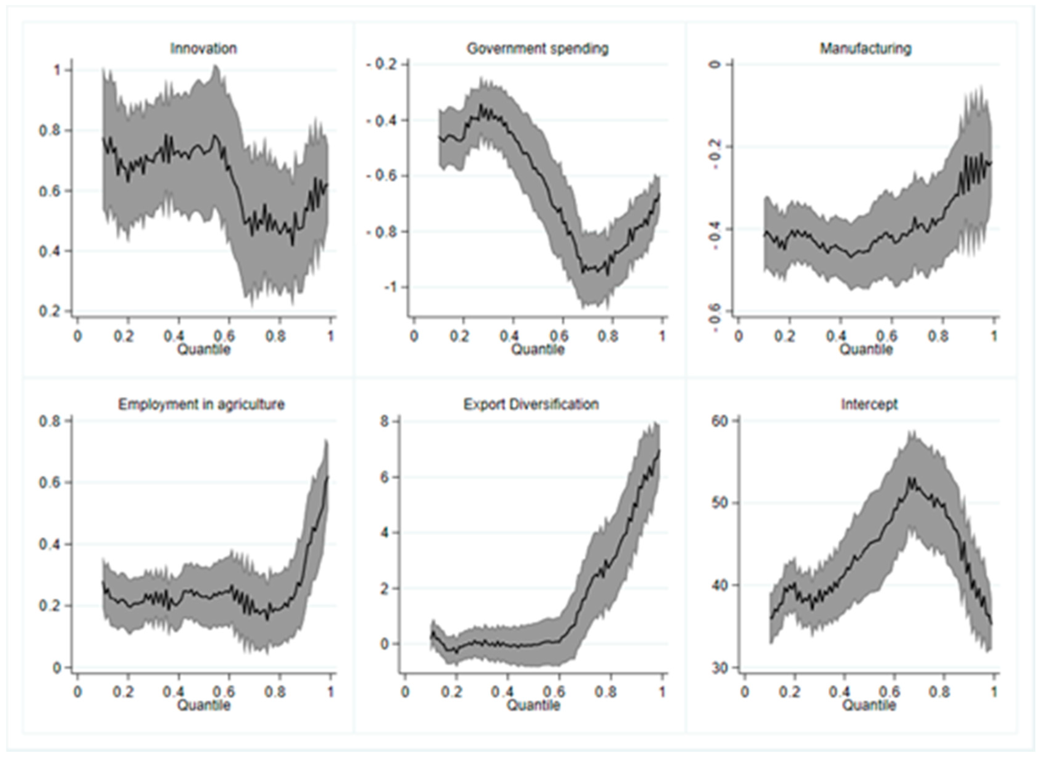
Figure 4 shows that the quantile distribution of the MHICs varies among the other groups. Innovation and manufacturing show an increase in inequality in the first quantiles, which then tends to decrease in the last ones. However, public spending tends to increase as the analysis quantiles increase. In the employment in agriculture and the diversification of exports, an almost constant trend is identified with negative values throughout the distribution. 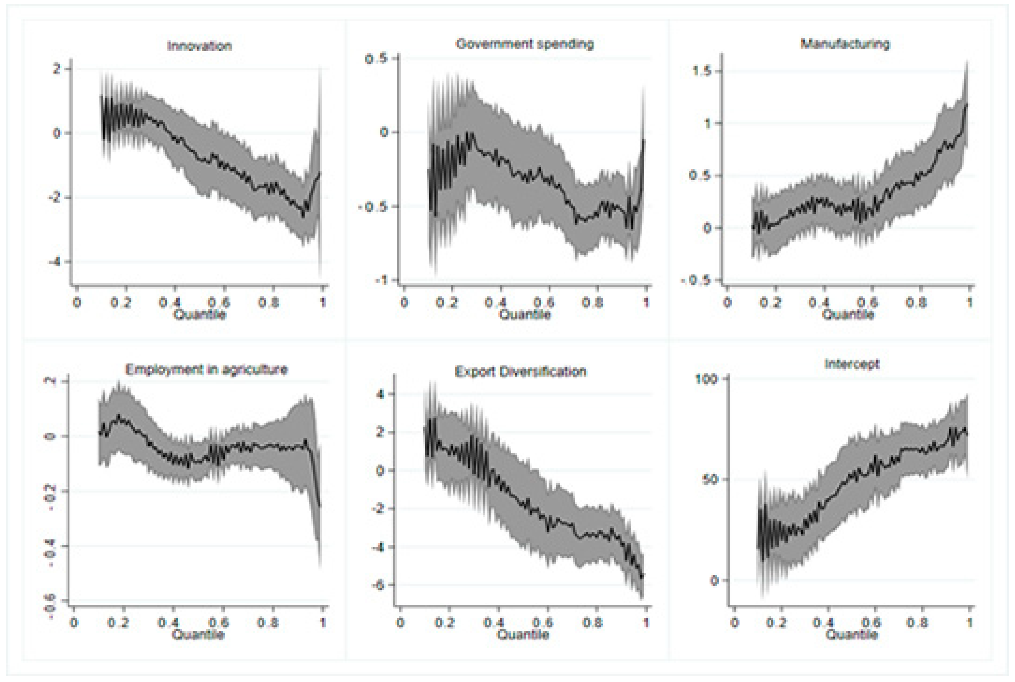Figure 5 reports the quantile regression sequence viewer for high-income countries. In the MLIC evidenced in Figure 6, it is evident that innovation and export diversification tend to reduce inequality to a greater extent at the end of the distribution. In public spending and employment in agriculture, inequality presents higher values in the first quantiles and decreases in the last ones. On the other hand, manufacturing is the only variable with a growing behavior in this group of countries, showing greater increases in inequality in the last quantiles. These results are due to the economic structure of each group of countries that causes an increase or decrease in inequality. Figure 7 illustrates the sequence display of the quantile regressions for lower-middle income countries.

Table 8. Results of the second-generation unit root tests.

Groups	Variables	Herwartz and Siedenburg (2008) [72]		Pesaran (2007) [81]		Breitung (2000) [71]
		Levels	Second Difference	Levels	Second Difference	Levels	Second Difference
73 countries	Inequality	−0.72	−3.28 ***	−2.21 ***	−6.06 ***	2.12	−2.86 ***
	Innovation	−0.40	−3.26 ***	−1.90	−5.87 ***	1.39	−4.33 ***
	Government spending	−1.54	−2.58 **	−1.80	−5.75 ***	−1.35	−5.11 ***
	Manufacturing	−1.19	−1.99 *	−2.05 *	−5.91 ***	−1.89	−6.78 ***
	Employment in agriculture	3.09	−3.17 ***	−2.33 ***	−5.77 ***	6.19	−5.02 ***
	Exports diversification	1.40	−2.23 **	−1.67	−5.78 ***	2.42	−5.76 ***
High income countries	Inequality	−2.42 **	−3.16 ***	−2.61 ***	−5.97 ***	−0.55	−2.77 **
	Innovation	−0.39	−3.10 ***	−2.46 ***	−5.70 ***	1.26	−3.46 **
	Government spending	−1.37	−2.61 **	−1.43	−5.76 ***	−0.91	−3.79 ***
	Manufacturing	0.73	−3.08 ***	−2.25 ***	−5.76 ***	1.64	−6.17 ***
	Employment in agriculture	1.92	−2.82 **	−2.31 ***	−6.04 ***	4.38	−4.29 ***
	Exports diversification	0.08	−2.01 **	−1.52	−5.83 ***	2.00	−4.96 ***
Middle-high income countries	Inequality	−0.17	−2.53 **	−2.99 ***	−6.05 ***	1.81	−1.50 *
	Innovation	−1.64 *	−2.81 **	−2.62 ***	−5.86 ***	−0.61	−2.82 **
	Government spending	−1.72 *	−2.58 **	−2.00	−5.75 ***	−1.14	−2.91 **
	Manufacturing	−1.33	−2.62 **	−1.33	−5.99 ***	1.19	−3.36 ***
	Employment in agriculture	2.85	−2.73 **	−1.76	−5.65 ***	2.57	−2.66 **
	Exports diversification	1.83	−2.10 **	−2.00	−5.68 ***	1.16	−2.58 **
Middle-low income countries	Inequality	−0.42	−2.61 **	−3.03 ***	−5.99 ***	2.89	−0.81
	Innovation	1.28	−2.11 **	−1.74	−6.02 ***	2.36	−1.23
	Government spending	−0.66	−2.06 **	−1.74	−5.98 ***	−0.21	−2.02 **
	Manufacturing	−1.24	−2.34 **	−2.26 **	−6.01 ***	−0.06	−2.21 **
	Employment in agriculture	2.06	−2.55 **	−2.00	−5.50 ***	3.69	−1.69 *
	Exports diversification	−1.44	−2.18 **	−1.53	−6.17 ***	0.84	−2.47 **

Note: The *, **, *** denotes significance at 0.1%, 1% and 5%, respectively.

reports the characteristics of the data concerning the temporal dimension. Once the presence of cross-dependence in the cross-sections was determined, the second-generation unit root tests of Herwartz and Siedenburg [72], Pesaran [81], and Breitung [71] were used. Upon analyzing the results, the three tests agree that in most of the variables in the levels, the null hypothesis stating that the series has a unit root is not rejected. However, when their second difference is already obtained, the variables lose their trend component, and it is possible to reject the said hypothesis. That is why the variables correspond to an integration I (2) order at 1% and 5% significance.

Using the Westerlund cointegration test [73], the results indicated in

Table 9. Results of the Westerlund cointegration test (2007).

	Statistic	Value	Z-Value	p-Value	Robust p-Value
73 countries	Gt	−3.94 ***	−14.65	0.00	0.00
	Ga	−7.04	5.21	1.00	0.50
	Pt	−37.52 ***	−17.55	0.00	0.00
	Pa	−7.90 ***	0.14	0.56	0.00
High income countries	Gt	−3.88 ***	−9.79	0.00	0.00
	Ga	−6.08	4.35	1.00	0.60
	Pt	−25.10 ***	−11.43	0.00	0.00
	Pa	−8.77	−0.55	0.29	0.06
Middle-high income countries	Gt	−4.28 ***	−9.60	0.00	0.00
	Ga	−8.01 ***	2.27	0.99	0.00
	Pt	−17.49 ***	−7.09	0.00	0.00
	Pa	−8.23 ***	−0.12	0.45	0.00
Middle-low income countries	Gt	−3.61 ***	−5.55	0.00	0.00
	Ga	−7.82	2.03	0.98	0.16
	Pt	−19.47 ***	−9.77	0.00	0.00
	Pa	−7.50	0.27	0.61	0.12

Note: The *** denotes significance at 5%.

were obtained. In the said test, the four statistics that revealed the existence of cointegration for the group and the panel were shown. Consequently, the Gt and Ga statistics indicated that at least one panel is cointegrated and that Pt and Pa determined the cointegration in the entire panel. It is established that the four statistics are significant at 1% only in the MHICs. At a global level and in the other groups, the short-term equilibrium is fulfilled in most of the statistics. These results reflect that the null hypothesis of no cointegration is rejected, and it is concluded that cointegration does exist. This means that the variables move together and simultaneously; in other words, the independent variables generate immediate changes or impacts on inequality.

Our results differ from the contribution of Glomm and Ravikumar [33], who stipulated that public spending does not reduce inequality in the short term. Implementing equitable policies in the educational sphere is not significant as the gap between the population with high and low incomes widens. Investment in human capital entails a long-term vision in terms of productivity and is therefore significant. Similarly, efficiency in public spending is key to reducing inequality. This scenario is more evident in developed countries that prioritize the population’s welfare [40], unlike developing countries, where a relationship exists in the short run but disappears in the long term [45]. When there is a low allocation to public spending, which is not sustainable over time, its inequality-reducing effect is not satisfactorily fulfilled. In the rest of the variables, no empirical evidence has analyzed their behaviors with inequality in the short term.

Table 10. Short-run elasticity.

	Panel AMG				Panel CCE-MG
	73 Countries	HIC	MHIC	MLIC	73 Countries	HIC	MHIC	MLIC
Innovation	−2.70	−3.09	−0.23	−1.56	−2.20	−3.02	−0.34	−1.9
	(−1.63)	(−1.62)	(−0.24)	(−0.87)	(−1.37)	(−1.38)	(−0.43)	(−0.77)
Government spending	0.60	0.82 *	0.22	0.36	0.36	0.47	−0.02	0.91
	(1.77)	(2.30)	(0.91)	(0.63)	(1.16)	(1.73)	(−0.10)	(1.12)
Manufacturing	−0.43	0.04	−0.43	−1.67	−0.50	0.02	−0.43	−1.32
	(−0.94)	(0.15)	(−1.01)	(−1.18)	(−1.26)	(0.08)	(−1.37)	(−1.47)
Employment in agriculture	0.79	0.50	0.02	0.59	0.49	−0.48	0.11	−0.18
	(1.53)	(0.71)	(0.05)	(0.92)	(1.42)	(−0.61)	(0.34)	(−0.69)
Exports diversification	2.35	−1.27	1.73	4.90	0.492	−0.91	4.15	−2.04
	(0.73)	(−0.55)	(0.72)	(0.59)	(0.24)	(−0.71)	(1.52)	(−0.28)
c_d_p					1.13 **	1.10 ***	1.21 ***	0.99 *
					(3.14)	(3.54)	(3.37)	(2.10)
Inequality _avg	0.76	1.20 ***	1.11 **	1.45
	(1.83)	(3.80)	(3.24)	(1.72)
Innovation _avg	−1.01	6.91 *	3.55	−3.44
	(−0.29)	(2.07)	(0.85)	(−0.61)
Government spending _avg	−1.09 *	−1.37 **	−0.16	0.61
	(−2.43)	(−2.61)	(−0.18)	(0.53)
Manufacturing _avg	−0.36	−0.95	0.34	−1.06
	(−0.51)	(−1.57)	(0.82)	(−0.95)
Employment in agriculture _avg	1.12	0.27	0.11	0.19
	(0.97)	(0.28)	(0.17)	(0.31)
Exports diversification _avg	−4.61	0.59	−0.28	6.75
	(−1.29)	(0.19)	(−0.06)	(0.45)
Constant	0.005	0.03	0.03	−0.03	−0.05	−0.40 ***	−2.28 ***	0.80
	(0.19)	(1.36)	(0.74)	(−0.38)	(−1.69)	(−3.52)	(−3.36)	(1.91)
Observations	1679	805	506	368	1679	805	506	368
Countries (N)	73	35	22	16	73	35	22	16
Chi-squared	7.01	8.59	2.87	5.85	6.02	5.52	5.35	2.64

Note: t statistics in parentheses * p < 0.05, ** p < 0.01, *** p < 0.001.

reports the short-term elasticities using the AMG and CCE-MG models. Short-run elasticities provide an early warning about the factors that affect inequality and deserve attention by policymakers to prevent the problem from exacerbating. In this sense, in the AMG panel, there is no statistical significance in any of the variables for each group analyzed in the short term, except for public spending that generates increases in inequality in the HICs. However, considering the average effect of the cross-sections, it is evident that innovation and public spending are already significant. In the case of innovation, its impact on inequality in the short term is positive for HICs. Unlike the result shown at the top, the effect is negative on public spending. This fact makes economic sense since the countries with the highest development level have a high public expenditure on health and education. This result immediately affects access to greater opportunities that benefit the population. On the contrary, the expected sign is obtained in the other variables and the SCC-MG panel, but with a lack of statistical significance. This suggests that the coefficients do not generate a significant short-run elasticity on inequality.

The long-run elasticities indicate the cumulative effect of the regressor variables on inequality. Unlike the short-term elasticities, a greater statistical significance was identified. Innovation has a significant negative relationship with long-term inequality in HICs and MLICs. This fact was corroborated by Canh et al. [28] by establishing that innovation through the promotion of the internet and mobile diffusion reduce inequality in the short and long terms. Public spending is also statistically significant at the global level, which for HICs and MLICs presents a positive effect. However, in the MHICs, the effect on inequality is negative. The results agree with Álvarez-Gálvez and Jaime-Castillo [43] on the inverse and significant long-term relationship between social spending and inequality. On the other hand, this result contradicts the expected sign since, as demonstrated by Gruber and Kosack [38] and Hanewald et al. [46], the budget headings in public spending and the efficiency in managing said expenditure determine its incidence of inequality. Manufacturing increases inequality in HICs while reducing inequality in MHICs and MLICs. Due to their higher industrial level, developing countries contribute to improving their economic development. Even so, Liu [47] extolled that the industry’s positive effect on inequality occurs until a turning point is reached, and from there, it tends to decrease.

Table 11. Long-run elasticity.

	Panel-FMOLS		Panel-DOLS
	Coefficient	t-Statistic	Coefficient	t-Statistic
73 countries
Innovation	−1.78	1.20	3.06	0.74
Government spending	0.35 *	6.97	0.52 *	1.98
Manufacturing	−0.16	−0.76	−0.10	−0.66
Employment in agriculture	0.68 *	5.22	−0.22 *	−2.42
Exports diversification	0.01 *	6.97	−8.32 *	−5.68
High income countries
Innovation	−2.79 *	−2.44	3.38	1.13
Government spending	0.42 *	3.82	0.16	0.16
Manufacturing	0.25 **	7.04	−0.80	−1.71
Employment in agriculture	1.56 *	5.33	1.04	−1.52
Exports diversification	0.14	1.18	−5.11 *	−2.98
Middle-high income countries
Innovation	−0.53	−1.56	−0.91	−0.03
Government spending	−0.40 *	−4.05	0.34	1.13
Manufacturing	−0.41 *	−5.34	−0.78	−1.63
Employment in agriculture	−0.16 *	−2.91	−0.71	0.62
Exports diversification	2.34 **	7.05	−4.04 *	−2.11
Middle-low-income countries
Innovation	−1.29 **	8.01	7.83	−0.05
Government spending	1.22 **	14.00	1.56 *	2.65
Manufacturing	−0.70 **	−5.78	2.37 *	3.03
Employment in agriculture	−0.10 **	6.68	−2.29 *	−3.65
Exports diversification	−3.48 **	4.87	−21.24 *	−5.25

Note: The * and **, denotes significance at 0.1% and 1%, respectively.

reports the long-run elasticities using the FMOLS and DOLS models. For its part, employment in agriculture increases inequality globally and in HICs. In contrast, the effect on the 73 countries jointly with the Dynamic Ordinary Least Squares is negative. In middle-income countries, this variable decrease inequality due to the economic activities in which the inhabitants of said countries are engaged. Bou et al. [53] emphasized that the income derived from agricultural activities in developing countries is more significant than that obtained by other sectors. Finally, the diversification of exports increases inequality at the global and MHIC levels in insignificant amounts. Although with DOLS, the negative effect is relevant for all groups of countries, causing a notable reduction in inequality. When nations diversify their commercial offerings, they are more competent. Government authorities can repay the population with better income distribution by obtaining a higher income. Le et al. [20] also found a long-term relationship between export diversification and inequality.

Table 12. Results of Dumitrescu-Hurlin panel causality test.

Relation	Statistic	73 Countries	HIC	MHIC	MLIC
$\mathrm{Inequality}\to$ innovation	Z-bar	2.52	0.51	2.03	2.26 *
	p-value	(0.14)	(0.61)	(0.09)	(0.05)
Innovation $\to$ Inequality	Z-bar	6.29 ***	1.62	1.33	9.48 ***
	p-value	(0.00)	(0.23)	(0.26)	(0.00)
Inequality $\to$ government spending	Z-bar	4.52	−0.16	0.89	8.85 ***
	p-value	(0.06)	(0.92)	(0.47)	(0.00)
Government spending $\to$ Inequality	Z-bar	2.43	−0.04	1.01	4.07 **
	p-value	(0.15)	(1.00)	(0.38)	(0.01)
Inequality $\to$ manufacturing	Z-bar	8.14 ***	0.65	8.84 ***	6.06 ***
	p-value	(0.00)	(0.62)	(0.00)	(0.00)
Manufacturing $\to$ Inequality	Z-bar	3.17 *	0.88	4.27 **	0.47
	p-value	(0.05)	(0.57)	(0.01)	(0.74)
Inequality $\to$ employment in agriculture	Z-bar	0.71	1.57	0.07	−0.89
	p-value	(0.62)	(0.23)	(0.92)	(0.49)
Employment in agriculture $\to$ Inequality	Z-bar	2.82	2.52	−0.96	3.43 *
	p-value	(0.11)	(0.13)	(0.39)	(0.04)
Inequality $\to$ exports diversification	Z-bar	2.77	1.69	3.07	−0.18
	p-value	(0.14)	(0.29)	(0.06)	(0.91)
Exports diversification $\to$ Inequality	Z-bar	3.93 *	2.05	1.84	3.20 *
	p-value	(0.05)	(0.16)	(0.20)	(0.02)

Note: The *, ** and *** denotes significance at 0.1%, 1% and 5%, respectively.

reports the Dumitrescu and Hurlin [79] causality test results. The results are grouped into two stages. Firstly, the bidirectional results offer a comprehensive view of a mutual causality of the series. In this group, there is a causal relationship in both directions between inequality and innovation in the MLICs. The bidirectionality between public spending and inequality is included for the same group of countries. In the second part, the results of the unidirectional relationships are integrated. At a global level, innovation causes inequality in a significant way. In the MLICs, inequality causes manufacturing and agriculture employment and export diversification. Given that most of the independent variables are the ones that cause inequality, it is essential to implement policies that counteract this problem.

These findings reflect that innovation leads to inequality due to the differences in the economic sectors in the countries [24]. Public spending turns out to be significant only in a group of countries. In developing economies, public investment contributes to reducing inequality only in certain regions due to the various public spending instruments that are usually applied [34]. Manufacturing has a two-way impact on lower-income countries. The development of the industrial sector for these nations is low; therefore, they are the most affected in terms of inequality [48]. Employment in agriculture and export diversification does not have a significant causal relationship due to the productive and commercial structure of the countries. In the same way, the gap between the center and the periphery remains in force, hindering a better economic outlook in all countries [56].

6. Conclusions and Policy Implications

This research examined the link between technological innovation and income inequality worldwide in a panel of 73 countries. To obtain a robust model, public spending, manufacturing, agricultural employment, and the export diversification index were included. The findings showed that, on average, innovation increases inequality both globally and in high-income countries. In contrast, public spending and agricultural employment have a negative impact on inequality in all groups. Unlike manufacturing, which increases inequality in the MLICs, the diversification of exports reduces it in this group of countries. The quantile regressions showed that at the global level and in the HICs, public spending and manufacturing reduce inequality throughout the distribution. Similarly, the negative effect for all quantiles is caused by agricultural employment and export diversification in the MHICs. The rest of the variables present heterogeneous effects in the deciles for each group of countries. In addition, the presence of cointegration between the study variables was confirmed. However, there was evidence of a lack of short-term elasticity in both estimators, even though in the long run innovation was constituted as a factor that reduced inequality. The other variables show a positive effect at the global and HIC levels; in middle-income countries, the effect is negative. Causality indicated a unidirectional causal relationship from the explanatory variables to inequality. However, the hypotheses raised through the various methodologies were verified.

Policymakers must implement projects and programs that foster innovation through a more significant number of patents that contribute to economic development and reduce inequality. This fact is linked to a greater allocation of public expenditure on education in budget plans in such a way as to guarantee the increase in human capital as the basis for innovation. In turn, this will allow for improved knowledge and technological developments that will also reduce the inequality of opportunities. Since manufacturing reduces inequality in developed countries, transitioning from an agricultural economy to an industrialized economy through increased spending on R&D is necessary. Even the provision of a better infrastructure with a greater investment of fixed capital would be a factor that would contribute to improved development. The impact of agricultural employment differs across countries due to their different levels of development. Therefore, the productive activities of developing economies are concentrated in the agricultural or livestock sector. In developed economies, employment is allocated to the industrial or services sector. Thus, with the impact of the export diversification index, this research recommends diversifying the commercial offer that promotes the competitiveness of the countries. From there, more income would be captured for the countries and distributed to the population towards efficient social projects that reduce inequality.

We believe that, within the near future, the negative impact of technological innovation on inequality will not significantly change for two reasons. Firstly, the countries, universities, and companies that are innovating will continue to do so for the foreseeable future. Therefore, the link between the two variables may remain stable in the coming years. However, future research should consider incorporating institutional variables on access to innovation and the externalities of the benefits of technological progress.

References

1. Odhiambo, N.M. Information technology, income inequality and economic growth in sub-Saharan African countries. Telecommun. Policy 2022, 46, 102309. [Google Scholar] [CrossRef]
2. Law, S.H.; Naseem, N.; Lau, W.T.; Trinugroho, I. Can innovation improve income inequality? Evidence from panel data. Econ. Syst. 2020, 44, 100815. [Google Scholar] [CrossRef]
3. Gravina, A.F.; Lanzafame, M. Finance, globalisation, technology and inequality: Do nonlinearities matter? Econ. Model. 2020, 96, 96–110. [Google Scholar] [CrossRef]
4. de Mendonça, H.F.; Baca, A.C. Fiscal opacity and reduction of income inequality through taxation: Effects on economic growth. Q. Rev. Econ. Financ. 2021, 83, 69–82. [Google Scholar] [CrossRef]
5. Medeiros, M.; Barbosa, R.J.; Carvalhaes, F. Educational expansion, inequality and poverty reduction in Brazil: A simulation study. Res. Soc. Strat. Mobil. 2019, 66, 100458. [Google Scholar] [CrossRef]
6. Fosu, A.K. Growth, inequality, and poverty reduction in developing countries: Recent global evidence. Res. Econ. 2017, 71, 306–336. [Google Scholar] [CrossRef] [Green Version]
7. Kitaura, K.; Miyazawa, K. Inequality and conditionality in cash transfers: Demographic transition and economic development. Econ. Model. 2020, 94, 276–287. [Google Scholar] [CrossRef]
8. Patel-Campillo, A.; García, V.S. Breaking the poverty cycle? Conditional cash transfers and higher education attainment. Int. J. Educ. Dev. 2022, 92, 102612. [Google Scholar] [CrossRef]
9. Mookherjee, D.; Napel, S. Welfare rationales for conditionality of cash transfers. J. Dev. Econ. 2021, 151, 102657. [Google Scholar] [CrossRef]
10. Bilbiie, F.O.; Känzig, D.R.; Surico, P. Capital and income inequality: An aggregate-demand complementarity. J. Monet. Econ. 2022, 126, 154–169. [Google Scholar] [CrossRef]
11. Hu, Z. The effect of income inequality on human capital inequality: Evidence from China. Struct. Chang. Econ. Dyn. 2021, 58, 471–489. [Google Scholar] [CrossRef]
12. Alvarado, R.; Tillaguango, B.; López-Sánchez, M.; Ponce, P.; Işık, C. Heterogeneous impact of natural resources on income inequality: The role of the shadow economy and human capital index. Econ. Anal. Policy 2021, 69, 690–704. [Google Scholar] [CrossRef]
13. Jia, F.; Ma, X.; Xu, X.; Xie, L. The differential role of manufacturing and non-manufacturing TFP growth in economic growth. Struct. Chang. Econ. Dyn. 2019, 52, 174–183. [Google Scholar] [CrossRef]
14. Gabriel, L.F.; Ribeiro, L.C.D.S. Economic growth and manufacturing: An analysis using Panel VAR and intersectoral linkages. Struct. Chang. Econ. Dyn. 2019, 49, 43–61. [Google Scholar] [CrossRef]
15. Barua, A.; Ghosh, P. Factor specificity and wage inequality in a developing economy: The role of technology and trade in Indian manufacturing. Int. Rev. Econ. Financ. 2017, 52, 77–90. [Google Scholar] [CrossRef]
16. Anwar, S.; Sun, S. Trade liberalisation, market competition and wage inequality in China’s manufacturing sector. Econ. Model. 2012, 29, 1268–1277. [Google Scholar] [CrossRef] [Green Version]
17. Guo, D.; Jiang, K.; Xu, C.; Yang, X. Industrial clustering, income and inequality in rural China. World Dev. 2022, 154, 105878. [Google Scholar] [CrossRef]
18. Gyapong, A.Y. How and why large scale agricultural land investments do not create long-term employment benefits: A critique of the ‘state’ of labour regulations in Ghana. Land Use Policy 2020, 95, 104651. [Google Scholar] [CrossRef]
19. Maisonnave, H.; Mamboundou, P.N. Agricultural economic reforms, gender inequality and poverty in Senegal. J. Policy Model. 2022, 44, 361–374. [Google Scholar] [CrossRef]
20. Işcan, T.B.; Lim, K.M. Structural transformation and inequality: The case of South Korea. Econ. Model. 2021, 107, 105735. [Google Scholar] [CrossRef]
21. Le, T.-H.; Nguyen, C.P.; Su, T.D.; Tran-Nam, B. The Kuznets curve for export diversification and income inequality: Evidence from a global sample. Econ. Anal. Policy 2019, 65, 21–39. [Google Scholar] [CrossRef]
22. Butler, A.; Dueker, M. Does foreign innovation affect domestic wage inequality? J. Int. Econ. 1999, 47, 61–89. [Google Scholar] [CrossRef]
23. Arocena, R.; Sutz, J. Inequality and innovation as seen from the South. Technol. Soc. 2003, 25, 171–182. [Google Scholar] [CrossRef]
24. Fukiharu, T. Income distribution inequality, globalization, and innovation: A general equilibrium simulation. Math. Comput. Simul. 2013, 93, 117–127. [Google Scholar] [CrossRef]
25. Ojha, V.P.; Pradhan, B.K.; Ghosh, J. Growth, inequality and innovation: A CGE analysis of India. J. Policy Model. 2013, 35, 909–927. [Google Scholar] [CrossRef]
26. Chu, A.C.; Cozzi, G.; Furukawa, Y. Unions, innovation and cross-country wage inequality. J. Econ. Dyn. Control. 2016, 64, 104–118. [Google Scholar] [CrossRef] [Green Version]
27. Frydman, C.; Papanikolaou, D. In search of ideas: Technological innovation and executive pay inequality. J. Financ. Econ. 2018, 130, 1–24. [Google Scholar] [CrossRef] [Green Version]
28. Canh, N.P.; Schinckus, C.; Thanh, S.D.; Ling, F.C.H. Effects of the internet, mobile, and land phones on income inequality and The Kuznets curve: Cross country analysis. Telecommun. Policy 2020, 44, 102041. [Google Scholar] [CrossRef]
29. Drummond-Lage, A.P.; da Veiga, C.R.P.; da Veiga, C.P.; de Melo, A.C.; Wainstein, A.J.A. Can innovation increase the therapeutic options but accentuate the inequalities in the healthcare system? J. Cancer Policy 2020, 25, 100237. [Google Scholar] [CrossRef]
30. Madsen, J.; Strulik, H. Technological change and inequality in the very long run. Eur. Econ. Rev. 2020, 129, 103532. [Google Scholar] [CrossRef]
31. Prettner, K.; Strulik, H. Innovation, automation, and inequality: Policy challenges in the race against the machine. J. Monet. Econ. 2019, 116, 249–265. [Google Scholar] [CrossRef]
32. Adams, S.; Akobeng, E. ICT, governance and inequality in Africa. Telecommun. Policy 2021, 45, 102198. [Google Scholar] [CrossRef]
33. Glomm, G.; Ravikumar, B. Public education and income inequality. Eur. J. Politi. Econ. 2003, 19, 289–300. [Google Scholar] [CrossRef]
34. Zhang, X.; Fan, S. Public investment and regional inequality in rural China. Agric. Econ. 2004, 30, 89–100. [Google Scholar] [CrossRef]
35. Anderson, L.R.; Mellor, J.M.; Milyo, J. Inequality and public good provision: An experimental analysis. J. Socio Econ. 2008, 37, 1010–1028. [Google Scholar] [CrossRef] [Green Version]
36. Glomm, G.; Kaganovich, M. Social security, public education and the growth–inequality relationship. Eur. Econ. Rev. 2007, 52, 1009–1034. [Google Scholar] [CrossRef]
37. Rajkumar, A.S.; Swaroop, V. Public spending and outcomes: Does governance matter? J. Dev. Econ. 2008, 86, 96–111. [Google Scholar] [CrossRef] [Green Version]
38. Gruber, L.; Kosack, S. The Tertiary Tilt: Education and Inequality in the Developing World. World Dev. 2014, 54, 253–272. [Google Scholar] [CrossRef] [Green Version]
39. Herrington, C.M. Public education financing, earnings inequality, and intergenerational mobility. Rev. Econ. Dyn. 2015, 18, 822–842. [Google Scholar] [CrossRef]
40. Dufrechou, P.A. The efficiency of public education spending in Latin America: A comparison to high-income countries. Int. J. Educ. Dev. 2016, 49, 188–203. [Google Scholar] [CrossRef]
41. Shen, K.; Wang, F.; Cai, Y. Patterns of inequalities in public transfers by gender in China. J. Econ. Ageing 2016, 8, 76–84. [Google Scholar] [CrossRef] [PubMed] [Green Version]
42. Bhattacharjee, A.; Shin, J.K.; Subramanian, C.; Swaminathan, S. Healthcare investment and income inequality. J. Health Econ. 2017, 56, 163–177. [Google Scholar] [CrossRef] [PubMed] [Green Version]
43. Álvarez-Gálvez, J.; Jaime-Castillo, A.M. The impact of social expenditure on health inequalities in Europe. Soc. Sci. Med. 2018, 200, 9–18. [Google Scholar] [CrossRef]
44. D’Agostino, G.; Pieroni, L.; Scarlato, M. Social transfers and income inequality in OECD countries. Struct. Chang. Econ. Dyn. 2019, 52, 313–327. [Google Scholar] [CrossRef]
45. Fuinhas, J.A.; Koengkan, M.; Santiago, R. Concentration hurts: Exploring the effects of capital stock on Latin American and Caribbean income inequality. J. Phys. Cap. Dev. Energy Transit. Lat. Am. Caribbean. 2021, 37–65. [Google Scholar] [CrossRef]
46. Hanewald, K.; Jia, R.; Liu, Z. Why is inequality higher among the old? Evidence from China. China Econ. Rev. 2021, 66, 101592. [Google Scholar] [CrossRef]
47. Liu, D. International trade and wage inequality: A non-monotonic relationship. Econ. Lett. 2013, 121, 244–246. [Google Scholar] [CrossRef]
48. Mehic, A. Industrial employment and income inequality: Evidence from panel data. Struct. Chang. Econ. Dyn. 2018, 45, 84–93. [Google Scholar] [CrossRef]
49. Borrs, L.; Knauth, F. Trade, technology, and the channels of wage inequality. Eur. Econ. Rev. 2020, 131, 103607. [Google Scholar] [CrossRef]
50. Mishra, A.; El-Osta, H.; Gillespie, J.M. Effect of agricultural policy on regional income inequality among farm households. J. Policy Model. 2009, 31, 325–340. [Google Scholar] [CrossRef]
51. El Benni, N.; Finger, R. The effect of agricultural policy reforms on income inequality in Swiss agricultura—An analysis for valley, hill and mountain regions. J. Policy Model. 2013, 35, 638–651. [Google Scholar] [CrossRef]
52. Ding, S.; Meriluoto, L.; Reed, W.R.; Tao, D.; Wu, H. The impact of agricultural technology adoption on income inequality in rural China: Evidence from southern Yunnan Province. China Econ. Rev. 2011, 22, 344–356. [Google Scholar] [CrossRef]
53. Dib, J.B.; Alamsyah, Z.; Qaim, M. Land-use change and income inequality in rural Indonesia. For. Policy Econ. 2018, 94, 55–66. [Google Scholar] [CrossRef]
54. Sutherland, L.-A. Agriculture and inequalities: Gentrification in a Scottish parish. J. Rural Stud. 2018, 68, 240–250. [Google Scholar] [CrossRef]
55. Klein, M.W.; Moser, C.; Urban, D.M. Exporting, skills and wage inequality. Labour. Econ. 2013, 25, 76–85. [Google Scholar] [CrossRef]
56. Hartmann, D.; Bezerra, M.; Lodolo, B.; Pinheiro, F.L. International trade, development traps, and the core-periphery structure of income inequality. EconomiA 2019, 21, 255–278. [Google Scholar] [CrossRef]
57. Kvedaras, V.; Cseres-Gergely, Z. China’s WTO accession and income inequality in European regions: External pressure and internal adjustments. Econ. Anal. Policy 2020, 69, 34–53. [Google Scholar] [CrossRef]
58. Zhu, S.; Yu, C.; He, C. Export structures, income inequality and urban-rural divide in China. Appl. Geogr. 2020, 115, 102150. [Google Scholar] [CrossRef]
59. Banco Mundial. Indicadores de Desarrollo Mundial (WDI). Available online: https://datos.bancomundial.org/indicator (accessed on 24 December 2021).
60. Pesaran, M.H.; Yamagata, T. Testing slope homogeneity in large panels. J. Econ. 2008, 142, 50–93. [Google Scholar] [CrossRef] [Green Version]
61. Blomquist, J.; Westerlund, J. Testing slope homogeneity in large panels with serial correlation. Econ. Lett. 2013, 121, 374–378. [Google Scholar] [CrossRef]
62. O’Connell, P.G. The overvaluation of purchasing power parity. J. Int. Econ. 1998, 44, 1–19. [Google Scholar] [CrossRef]
63. Pesaran, M.H. General diagnostic tests for cross-sectional dependence in panels. Empir. Econ. 2021. Available online: https://ideas.repec.org/p/ces/ceswps/_1229.html (accessed on 24 December 2021). [CrossRef]
64. Chudik, A.; Pesaran, M.H. Large panel data models with cross-sectional dependence: A survey. Worging Paper. 2013, 13, 15. [Google Scholar]
65. Pesaran, M.H. Testing Weak Cross-Sectional Dependence in Large Panels. Econ. Rev. 2014, 34, 1089–1117. [Google Scholar] [CrossRef] [Green Version]
66. Bailey, N.; Kapetanios, G.; Pesaran, M.H. Exponent of Cross-Sectional Dependence: Estimation and Inference. J. Appl. Econ. 2015, 31, 929–960. [Google Scholar] [CrossRef] [Green Version]
67. Koenker, R.; Bassett, G. Regression Quantiles. Econometrica 1978, 46, 33–50. [Google Scholar] [CrossRef]
68. Powell, D. Quantile Treatment Effects in the Presence of Covariates. Rev. Econ. Stat. 2020, 102, 994–1005. [Google Scholar] [CrossRef]
69. Chernozhukov, V.; Fernández-Val, I.; Melly, B. Quantile and Distribution Regression in Stata: Algorithms, Pointwise and Functional Inference. Available online: https://www.stata.com/meeting/switzerland20/slides/Switzerland20_Melly.pdf (accessed on 5 January 2022).
70. Powell, D. Quantile regression with nonadditive fixed effects. Empir. Econ. 2022, 1–17. [Google Scholar] [CrossRef]
71. Breitung, J. The Local Power of Some Unit Root Tests for Panel Data. In Nonstationary Panels, Panel Cointegration, and Dynamic Panels; Emerald Group Publishing Limited: Bingley, UK, 2000. [Google Scholar] [CrossRef] [Green Version]
72. Herwartz, H.; Siedenburg, F. Homogenous panel unit root tests under cross sectional dependence: Finite sample modifications and the wild bootstrap. Comput. Stat. Data Anal. 2008, 53, 137–150. [Google Scholar] [CrossRef]
73. Westerlund, J. Testing for Error Correction in Panel Data. Oxf. Bull. Econ. Stat. 2007, 69, 709–748. [Google Scholar] [CrossRef] [Green Version]
74. Persyn, D.; Westerlund, J. Error-Correction–Based Cointegration Tests for Panel Data. Stata J. Promot. Commun. Stat. Stata 2008, 8, 232–241. [Google Scholar] [CrossRef] [Green Version]
75. Cross-Section Dependence in Non-Stationary Panel Models: A Novel Estimator. Available online: https://mpra.ub.uni-muenchen.de/id/eprint/17692 (accessed on 5 January 2022).
76. Productivity Analysis in Global Manufacturing Production. Available online: https://ideas.repec.org/p/deg/conpap/c015_019.html (accessed on 5 January 2022).
77. Pesaran, M.H. Estimation and Inference in Large Heterogeneous Panels with a Multifactor Error Structure. Econometrica 2006, 74, 967–1012. [Google Scholar] [CrossRef] [Green Version]
78. Kapetanios, G.; Pesaran, M.H.; Yamagata, T. Panels with non-stationary multifactor error structures. J. Econ. 2011, 160, 326–348. [Google Scholar] [CrossRef] [Green Version]
79. Dumitrescu, E.-I.; Hurlin, C. Testing for Granger non-causality in heterogeneous panels. Econ. Model. 2012, 29, 1450–1460. [Google Scholar] [CrossRef] [Green Version]
80. Chen, B. Upstreamness, exports, and wage inequality: Evidence from Chinese manufacturing data. J. Asian Econ. 2017, 48, 66–74. [Google Scholar] [CrossRef]
81. Pesaran, M.H. A simple panel unit root test in the presence of cross-section dependence. J. Appl. Econ. 2007, 22, 265–312. [Google Scholar] [CrossRef] [Green Version]
82. Katz, L.F.; Murphy, K.M. Changes in Relative Wages, 1963–1987: Supply and Demand Factors. Q. J. Econ. 1992, 107, 35–78. [Google Scholar] [CrossRef]
83. Acemoglu, D.; Autor, D. Skills, Tasks and Technologies: Implications for Employment and Earnings. In Handbook of Labor Economics, 1st ed.; Ashenfelter, O., Card, D., Eds.; Elsevier: Amsterdam, The Netherlands, 2011; Volume 4, pp. 1043–1171. [Google Scholar] [CrossRef]
84. Autor, D.H.; Levy, F.; Murnane, R.J. The Skill Content of Recent Technological Change: An Empirical Exploration. Q. J. Econ. 2003, 118, 1279–1333. [Google Scholar] [CrossRef]
85. Acemoglu, D. Technical Change, Inequality, and the Labor Market. J. Econ. Lit. 2002, 40, 7–72. [Google Scholar] [CrossRef]
86. Acemoglu, D. Why Do New Technologies Complement Skills? Directed Technical Change and Wage Inequality. Q. J. Econ. 1998, 113, 1055–1089. [Google Scholar] [CrossRef] [Green Version]
Figure 1. Average values of the period of the variables.
Sustainability 14 08474 g001
Figure 2. Econometric process.
Sustainability 14 08474 g002
Figure 3. Quantile Plots of the model parameters.
Sustainability 14 08474 g003
Figure 4. Visualizing sequences of quantile regressions for distribution regression coefficients for 73 countries.
Sustainability 14 08474 g004
Figure 5. Visualizing sequences of quantile regressions for distribution regression coefficients for high income countries.
Sustainability 14 08474 g005
Figure 6. Visualizing sequences of quantile regressions or distribution regression coefficients for middle-high income countries.
Sustainability 14 08474 g006
Figure 7. Visualizing sequences of quantile regressions or distribution regression coefficients for middle-low income countries.
Sustainability 14 08474 g007