Comparing Micromobility with Public Transportation Trips in a Data-Driven Spatio-Temporal Analysis

Abstract

Micromobility service systems have recently appeared in urban areas worldwide. Although e-bike and e-scooter services have been operating for some time now, their characteristics have only recently been analyzed in more detail. In particular, the influence on the existing transportation services is not well understood. This study proposes a framework to gather data, infer micromobility trips, deduce their characteristics, and assess their relation to a public transportation network. We validate our approach by comparing it to similar approaches in the literature and applying it to data of over a year from the city of Aachen. We find hints at the recreational role of e-scooters and a larger commuting role for e-bikes. We show that micromobility services in particular are used in situations where public transportation is not a viable alternative, hence often complementing the available services, and competing with public transportation in other areas. This ambivalent relationship between micromobility and public transportation emphasizes the need for appropriate regulations and policies to ensure the sustainability of micromobility services.

1. Introduction and Motivation

In recent years, advancements in information and communications technology have enabled a digital transformation process. Two of the most prominent contributing factors to this ongoing process have been the worldwide prevalence of the Internet and the development of the first touchscreen smartphones in 2007. Nowadays, it has become customary for people to be connected to the Internet. This always-connected state enabled new business models and promoted progress in various areas. As such, digitalization also facilitated a change in the transportation sector. Until recently, transport modes could primarily be categorized as private or public transportation. Personal transportation such as a private car is often very flexible and quick in urban areas. In contrast, it made inefficient usage of available resources, such as a low average vehicle occupancy and a low utilization rate per time, and came with large space requirements. On the other hand, public transportation better uses the assigned resources in urban areas. However, it is often slower and more cumbersome due to its inflexibility and fixed stations and timetables. With digitalization, the gap between private and public transportation becomes more blurred: novel mobility modes such as car-, bike-, scooter-, and ride-sharing have become available to complement the available transportation modes. These novel modes, often summarized as micromobility, have in common that they are most often accessed with the traveler’s smartphone and offer personalized and flexible mobility services.

At the same time, global challenges such as urbanization and climate change have become more pressing. Climate change, fueled by the emission of greenhouse gases, is currently one of the leading global threats to the environment. Although greenhouse gas emissions have been stabilized in total in the European Union, the transportation sector emits the largest amount of greenhouse gases compared to other sectors, and it is the only sector in which emissions have continued to rise since 1990 [1]. Additionally, due to the ongoing urbanization process, more and more people are moving to cities. The United Nations expects $68\%$ of the world’s population to live in urban areas in 2050 [2], up from $55\%$ in 2019. Urbanization further stresses the often already congested and overcrowded transportation systems. This development shows that current urban transportation systems are neither sustainable from an ecological nor a transportation-oriented point of view; thus viable alternatives must be developed.

In an attempt to reduce carbon emissions in the transportation sector, the internal combustion engine of vehicles is currently being replaced by electric motors. While this reduces greenhouse gas emissions, the congested transportation systems in urban areas do not benefit from this step, as the number of private vehicles remains equal. As such, ecologically sustainable transportation modes that also satisfy the mobility requirements of travelers need to be promoted and improved. The inflexibility of public transportation and the first-mile last-mile problem are primary hindrances to people not using public transport [3]. The first-mile last-mile problem describes the difficulty of reaching the departing station from a starting location and reaching the destination from one’s arrival station in public transit networks. With its spontaneous and ubiquitous availability in urban areas, micromobility may strongly reduce the first- and last-mile problem by allowing travelers to reach their public transport stops quickly. As such, micromobility may alleviate the gap in flexibility between private and public transportation and enable more people to switch to sustainable mobility modes by offering an alternative to personal vehicles.

Micromobility and sharing systems may play a pivotal role in building environmentally sustainable transportation systems in urban areas. The characteristics of station-based micromobility modes are already well investigated. Previous research has established that micromobility can draw travelers from all other transportation modes, hinting at the possibility of improving the sustainability of transportation systems. Although research into micromobility is gaining more interest, data-driven analyses of real-world datasets over a more extended period are still scarce according to a recent systematic literature review by [4]. In particular, the characteristics of micromobility trips and their impact on the environment and the transportation network have not been thoroughly researched on real-world datasets with data-driven methods. Hence, it is still unknown whether, in a real-world setting, micromobility complements public transportation or competes with it and which factors influence this relationship. This study presents the results of a holistic data-driven micromobility case study that first obtains a micromobility trip dataset from available public data shared by micromobility operators, analyses the inferred trips and finally compares the trips with the existing public transportation network.

This case study applies data-driven methods to a dataset obtained from three micromobility service providers over a year in Aachen, Germany and compares it to data obtained from the local public transportation company. The dataset consists of the crowdsourced availability and location of the vehicles in the Aachen in a 10-min resolution obtained from the micromobility operator’s API that we then transformed into a dataset obtaining the trips performed with the vehicles in order to analyse and visualize the trips. Two providers offer a dockless e-scooter service and one provider offers a docked e-bike service. We developed a novel algorithm for inferring and categorizing trips to obtain trips from this spatio-temporal timestamped dataset. The algorithm infers the origins and destinations of trips and their purpose depending on the location and the vehicle’s state of charge difference. This inference transforms the data from a temporal snaphsot representation into a structured relational dataset, improving the manageability of the data. We show that the data sampling and transformation process does not fundamentally change the data. Furthermore, the inference step ensures the reproducibility of this work in other regions, as all data we use in this work is often publicly available. Next, we analyze the fleet of vehicles and the spatial and temporal characteristics of the micromobility usage from both a demand-side and supply-side viewpoint. Finally, we investigate its role in first- and last-mile passenger transportation and hypothesize which kinds of micromobility trips are used in Aachen. Here, we particularly focus on the relation to public transportation. With the results, we hope to support further regulations and planning decisions regarding the future of e-scooters as a part of sustainable intermodal mobility networks.

The results of the characteristics of micromobility usage agree with studies performed before in other cities around the world, performed with operator data. Hence, we argue that inferring trips from a spatio-temporal dataset of micromobility vehicle locations is possible and also relatively insensitive to the sampling interval. The analysis highlights that e-scooters are typically used for shorter trips than e-bikes. Furthermore, the temporal and spatial usage characteristics indicate that e-scooters may be used more for recreational use, whereas e-bikes are also used for commuting to work. When analyzing the location and time of trips, we show that micromobility has the potential to compete with or complement public transportation depending on the characteristics of the transportation network. This result indicates that appropriate policies must be in place to ensure the sustainability of micromobility.

This paper’s remainder is structured as follows: Section 2 reviews recent literature on e-scooter- and bike-sharing data analysis. It focuses on case studies performed worldwide and discusses different trip-inference algorithms. Next, Section 3 introduces the approach and methodology of our approach. Here, we present the gathered dataset and the various steps of the data analysis pipeline. Afterward, we first analyze the characteristics of micromobility usage in Aachen with the introduced methods in Section 4. After understanding micromobility usage in Aachen, we analyze the impact of micromobility services on public transportation. Finally, Section 5 concludes this work and presents possibilities for further research.

2. Literature Review

In our research, we tackle the analysis of spatial and temporal characteristics of docked e-bikes and dockless e-scooters with a particular focus on their influence on the first mile and last mile of public transportation. For a broader literature review, we refer the reader to available surveys about the topic micromobility [4,5,6]. Reck et al. [7] and Heumann et al. [8] conducted thorough literature reviews for their research papers highlighting spatio-temporal e-scooter trip data analysis. Similar to the propagation of the novel mobility modes themselves, the research in micromobility primarily started with docked bikes [9], followed by dockless bicycles [10], continued with docked e-bikes [11], and finally reached dockless e-scooters [12]. Docked (e-)bicycle systems are already well researched, whereas shared dockless e-scooters have more recently appeared in cities worldwide [7]. Hence, this overview targets papers addressing more recent e-scooter research or research of e-bikes in conjunction with e-scooters.

Reck et al. [7] categorized related work regarding data analysis into demand-side and supply-side research. The supply-sided analysis covers, among other things, the (re-) distribution of vehicles, the analysis of charging trips, the profitability of the provider, and the management of the vehicle fleet. The supply-side analysis, therefore, has a strong micromobility operator-centered viewpoint. The demand-side view analyzes how users use services and which factors influence usage, taking a more user-specific perspective. Data-driven approaches assume that the actual usage of the services also corresponds to the demand, as actual demand is not measurable. As we infer trips based on the location and state of charge of vehicles, we have access to demand and supply data and, therefore, regard the distribution in time and space on both the demand-side and the supply-side in this review.

Table 1. List of data-driven e-scooters studies, categorized by continent, city, and publication year.

Continent	City	References
North America	Austin	[13,14,15,16,17,18,19]
	Atlanta	[20]
	Indianapolis	[21,22]
	Kansas City	[18]
	Louisville	[18,23,24]
	Minneapolis	[13,18]
	Portland	[18]
	Washington	[12,25,26,27,28,29]
Asia	Singapore	[30]
Europe	Berlin	[8,31]
	Stockholm, Paris, Madrid	[31]
	Zurich	[7,32]

gives an overview of the current focus of data-driven mobility studies. The data shows that the United States is currently a particular focus of micromobility research; studies performed in Asia or Europe have just recently emerged and are more scarce. There are two main reasons for this: First, e-scooters were earlier legalized in the United States, giving researchers earlier access to the data. Secondly, some micromobility datasets, such as the dataset from Austin, are publicly available online (https://doi.org/10.26000/030.000003 accessed on 5 March 2022), explaining the large number of studies focusing on Austin. In Europe and Asia, due to privacy concerns, such datasets are seldom publicly available, requiring the data to be gathered for each study.

Although e-scooter and e-bike sharing are inherently similar, the trip characteristics often differ in details. E-scooter trips are usually fairly short with a distance of around 650 m [12] to $2.6$ km [31]. On the other hand, e-bike trips are often used for longer trips of $2.6$ km [12] to $4.2$ km [25]. The longer trips are sometimes attributed to the higher comfort of e-bikes, which may also explain the higher mean speed of e-bike trips [17]. E-scooter usage is often associated with recreation [14,24]. In contrast, e-bikes usage usually peaks in the morning and the early evening, indicating a significant role in commuting [7,12]. Furthermore, trip destinations associated with workplaces have a higher trip count for weekdays but not on weekends or holidays [33]. The same effect cannot be observed for e-scooters. Nevertheless, some studies also find hints at commuting use for e-scooters [15]. Younes [27] compared dockless e-scooters with docked e-bikes and found significant differences between the modes, both temporally and spatially. Noland [19] and Mathew [21] found evidence of e-scooters and e-bike usage being negatively affected by weather factors such as low temperature, precipitation, and strong wind. E-scooters, however, are less affected by weather factors than e-bikes. Indeed, the current e-scooter usage is not fully understood, and studies in different cities have come to different conclusions.

When analyzing the studies in different cities, the properties of e-scooter trips differ from area to area, indicating a considerable influence of spatial factors. Huo et al. [18] compared the e-scooter usage in five cities in the United States. The temporal distribution of trips is similar, with peaks between 11:30 and 17:30. The authors note that these peak hours are atypical when compared to public transportation or private car travel. Zou et al. [26] investigated the influence of biking infrastructure on micromobility trips and discovered that roads with biking infrastructure increase the likelihood of the road being used in a micromobility trip. High usage of e-scooters has generally often been observed in the city center and next to university campuses [16,18,24]. Similarly, a more significant density of bus stops is related to more e-scooter trips [15,18,29]; however, whether e-scooter trips and bus stops are independent is not clear. Luo et al. [22] concludes that most e-scooter trips substitute walking or public transportation trips in Louisiana, hinting that e-scooter usage is independent of bus stop density, as bus trips can be replaced with e-scooter trips.

Research about the relationship between e-scooters and public transportation is scarce. Luo et al. [22] proposed a modeling framework for investigating the relationship between e-scooter sharing systems and public transportation. Similar frameworks have also been proposed for other modes, such as ride-sharing [34]. With the modeling framework, they have performed a use-case study in Indianapolis, Indiana, and concluded that depending on the spatial features, e-scooter trips both compete with existing modes and complement them in hours of non-service. In urban areas with a well-developed public transportation network, e-scooters often compete with the existing network, and e-scooter operators encourage this through their redistribution strategy by placing their vehicles near public transportation stops. Espinoza et al. [20] observed that e-scooters are not often used to access the public transportation system in Atlanta. In areas with underdeveloped public transportation, e-scooters often complemented the public transportation system and are seldom driven for the first mile and last mile to public transportation. The study of [35] in Warsaw, Poland came to a similar conclusion. E-scooters have a higher probability of replacing public transportation trips than shared bicycles. Nevertheless, the authors highlight the possibility of e-scooters to support public transportation. Zuniga-Garcxia et al. [36] observed that a better public transportation service decreases e-scooter demand and vice-versa. Ziedan et al. [37] performed a case study in Nashville, Tennessee. They have found only marginal effects of e-scooter sharing systems influencing the public transportation network at all. To summarize, the current research on the effects of e-scooter sharing systems on public transportation networks is still unclear. There are indicators that it can complement or compete with public transportation depending on different temporal and spatial factors.

When examining data-driven micromobility research, two kinds of datasets and approaches emerge. For the first approach, aggregated trip data obtained from the operator is used for the analysis. This approach has the advantage that the trips are already computed and can be assumed to be correct, but it has the disadvantage that these trips are often aggregated to traffic analysis zones due to privacy concerns [14]. Often such studies focus on cities in the United States of America as the data is more readily publicly available there. In the other approach, researchers infer the trips from the API intended for the micromobility sharing application and compute the trips based on disappearing and reappearing trips in the data stream. Here, the advantage is that highly detailed data is available as more or less the exact location of the vehicles is known. However, the disadvantage is that the data will be noisier than data directly obtained from the operator as falsely identified trips are going to exist in the inferred dataset, whereas other trips will be missing all together. From the above mentioned data-driven micromobility studies, infer the trips based on the operator’s API [8,12,20,25,26,29,30,38], whereas the others analyze trip data directly obtained from the operator.

Xu et al. [28] propose multiple algorithms to extract trips from general bikeshare feed specification (GBFS) data. GBFS (https://github.com/NABSA/gbfs accessed on 5 March 2022) is a data format in which micromobility operators can publish their real-time data about their fleet. They distinguish between three kinds of vehicle IDs in their trip inference algorithm: a static ID, which stays constant for the whole observation period, a resetting ID which resets after each trip, and a dynamic ID that randomly changes. The simplest case is the static ID, where the sources of error are restricted to GPS measurement errors and the sample rate of obtaining the vehicle’s location from the API. For static IDs, it is possible to accurately reconstruct the data into trips, whereas for resetting it is possible to infer trips without assigning them to specific vehicles, and for dynamic IDs it is only possible to reconstruct unlinked trip origins and destinations. Our study works with static IDs; therefore, we can infer high-quality data. Heumann et al. [8] improved their trip inference algorithm to account for round, charging, and reallocation trips. Finally, Zhao et al. [32] analyzed the required sampling rate for reconstructing micromobility trips from the operator’s API. They validated different sampling rates and concluded that the sampling rate itself has only a minor influence on the data quality for most scenarios.

We identify several gaps in the current literature. Most of the literature focuses on data obtained from cities in the United States of America, as the data is often more readily available there. This means that micromobility is still not widely researched for European or Asian cities. This gap is problematic, as journey patterns could strongly diverge between different countries. Furthermore, the data used for analysis is often aggregated to traffic analysis zones due to privacy concerns, restricting the resolution with which the data can be examined. Lastly, the literature often only focuses on a single transportation mode. Some studies analyze multiple transportation modes [7,12,27]; however the influence on multiple micromobility with public transportation has not been well-researched. In particular, it is still unclear what influence micromobility has on public transportation and whether it replaces public transportation trips or whether it complements the service.

This paper attempts to address the identified gaps by proposing a framework to analyze micromobility trips obtained by polling the operator’s API. In this way, it is possible to obtain high-resolution data for most micromobility modes by querying widely available web services. This approach, therefore, fosters the transferability of the methodology to other regions, as it does not depend on a special dataset. To the best of our knowledge, the dataset covering trips over a whole year is the largest dataset obtained by querying the operator’s API up to date. Furthermore, we know of nearly no research attempting to assess the relationship between micromobility and public transportation with a data-driven method.

3. Approach

In the following section, we introduce the methodology of this work. First, we sketch the implemented data pipeline with the trip and public transit inference algorithms. Then we give an overview of the gathered dataset and the inferred fleet of micromobility in Aachen, Germany.

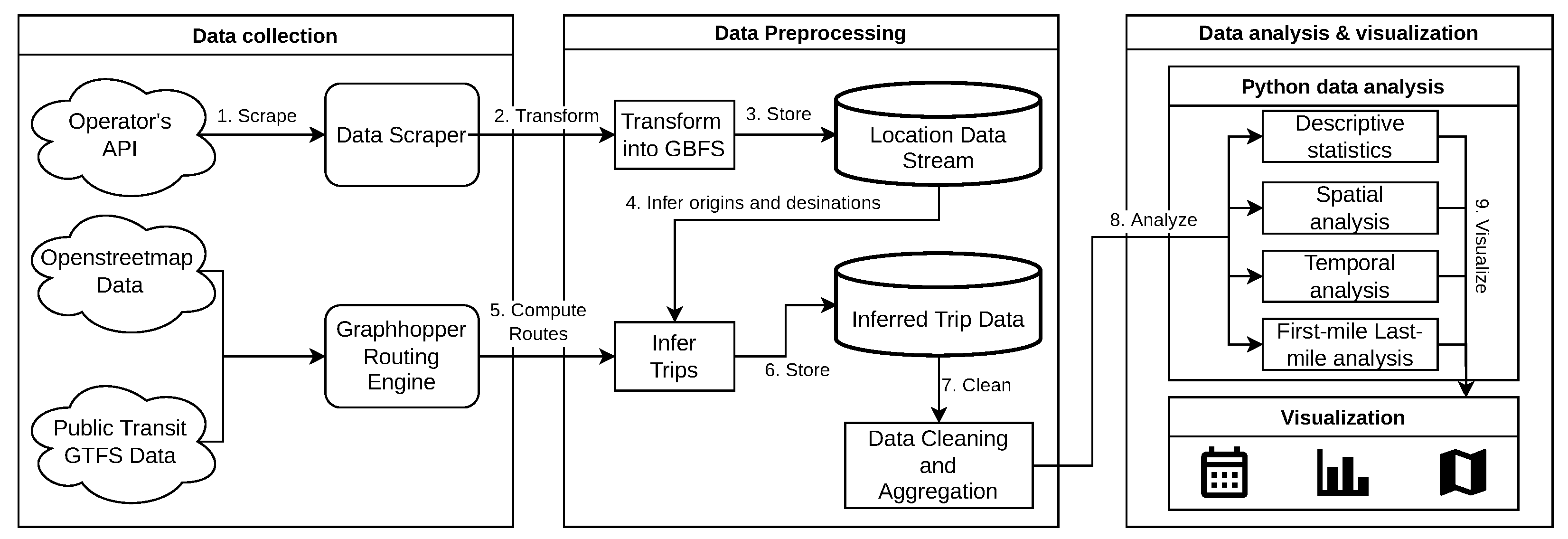
Figure 1 shows the developed data pipeline. In regular intervals, we obtain the vehicles’ location and state of charge from three micromobility operators in Aachen. We queried their APIs, which they also employ for their mobile information systems for customers. Therefore, the sketched approach is generalizable to all micromobility services, in which the operator offers an application that lists locations, availability, and the state of charge of their vehicles. As a second step, we clean the data and normalize the vendor-specific data format by transforming it into a GBFS-conforming dataset. We store this GBFS data into a time-series database with a resolution of 10 min.

From this time-series GBFS data, we infer the trips by comparing the differences between the snapshot logs. If a vehicle’s location drastically changes between two logs, we assume that a trip occurred between the snapshots. This inference step is mostly a data-transformation step and does not fundamentally change the data obtained from the operators. Depending on the characteristics of this inferred trip, we can assign a category to the trip; similar to [8], we differentiate between customer trips, charging trips, rebalancing trips, and deployment trips. Each inferred trip has an origin and destination and an approximate duration inferred by comparing the time difference between two logs. We calculate a probable routes with the Graphhopper routing engine (https://github.com/graphhopper/graphhopper accessed on 5 March 2022) by using a designed e-scooter routing profile to increase the computed route’s authenticity. The computed trips with their routes are then stored in a relational database for further analysis.

Before analyzing the trips, we further clean the data and discard implausible trips. The analysis consists of a descriptive analysis, where we investigate the fleets of the different mobility modes. Furthermore, we look at the number of active service days and the usage of the vehicles. Next, we regard spatial features of the trips and regions where the supply and demand are particularly significant. In the spatio-temporal analysis, we explore differences in trips depending on the time of day, the day in the week, and the month in the year. As a next step, we determine the influence of the trips on public transportation, depending on the trip’s spatial and temporal characteristics. Finally, we visualize all results with suitable visualization tools.

3.1. Data Collection and Trip Inference

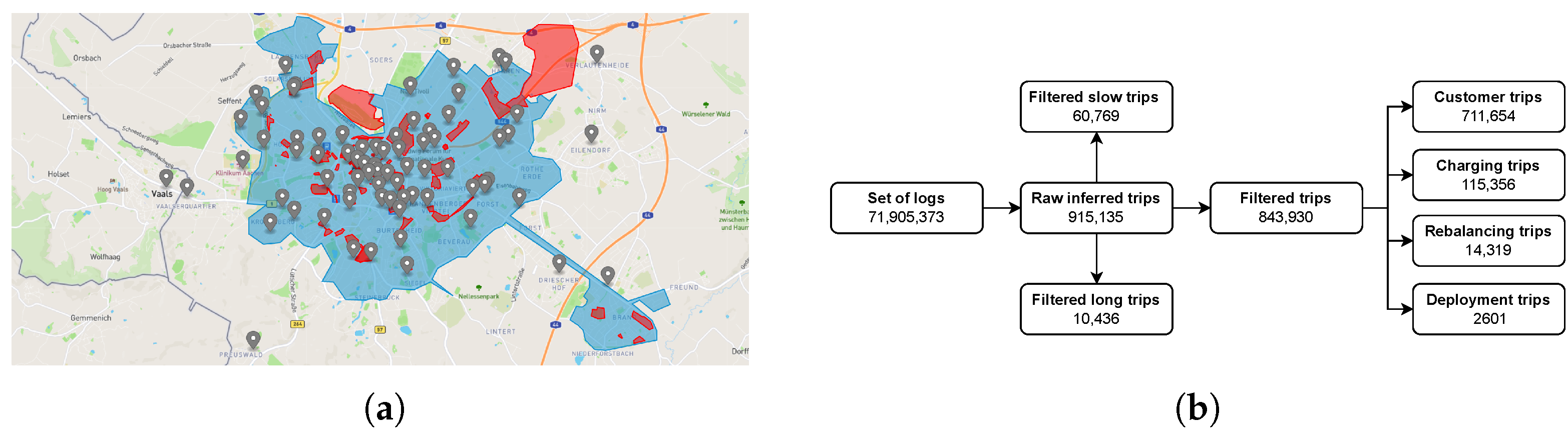
We have collected the micromobility trips from Aachen, Germany, from 4 December 2020, to 4 December 2021. Aachen is situated next to the border of The Netherlands and Belgium in the west of Germany and is a mid-sized city with 245,000 inhabitants and is overall fairly hilly. We chose Aachen as a city for this study, as it is a mid-sized city with many students and tourists. Students have different mobility patterns than other people, and in Aachen the biggest difference is that students can use public transportation free of charge. Tourists on the other hand also differ in their mobility behavior from regular residents. Next, most other studies have been performed in large cities with populations of several million people. Furthermore, Aachen was one of the first cities in Germany to have a diverse intermodal transportation network due to the project Mobility Broker, which integrated multiple transportation modes into a single platform. Hence, the data obtained in this study can help to better understand micromobility usage in mid-sized cities. The micromobility operators’ service area strongly focuses on the urban area of Aachen (see Figure 2a). We have obtained data points for around 55,000 time instants during the year, roughly corresponding to a data point every 10 min, totaling to approximately 72 million distinct data points for all vehicles. Figure 2b shows that a total of 900,000 raw trips have been inferred from that dataset. From this, we filtered trips that were either substantially too long or far too slow. We then categorized the resulting 850,000 trips based on their characteristics.

Algorithm 1 sketches the trip inference algorithm to infer the set of trips T from a set of logs L. The key idea of the algorithm is to use the disappearance and reappearance of vehicles in the data stream similar to other studies. If a vehicle disappears from the data stream and later reappears, or it significantly changes its location, it is likely that a trip has been conducted. As input, the algorithm receives the time of the first snapshot $t_{\mathrm{first}}$ and a set of logs L containing the vehicle’s location $l_k$ at time $t_k$ with state of charge $b_k$, vehicle id $\mathit{id}$ from operator $\mathit{op}$. Hence, we define a log as $l=(l_k,t_k,b_k,\mathit{op},\mathit{id})$ for a specific snapshot k. We define a trip $t\in T$ to have an origin $\mathit{or}$ and a destination $\mathit{dst}$ corresponding to the locations $l_k$ of two different logs. Analogously, a trip contains a start time $t_{\mathrm{start}}$ and an end time $t_{\mathrm{end}}$, which define the starting and ending time of the trip and are defined by the difference of time $t_k$ of two different logs. Furthermore, a trip has the battery difference for the trip $\Delta b$, set by the difference of the state of charge $b_k$ of two different logs. Lastly, a trip has the operator of the vehicle $\mathit{op}$, the vehicle id $\mathit{id}$ from the respective two logs $l_k$, and an inferred trip type type. Therefore, the set of trips T consists of trips $t=(\mathit{or},\mathit{dst},t_{\mathrm{start}},t_{\mathrm{end}},\Delta b,\mathit{op},\mathit{id},\mathit{type})$.

Algorithm 1 Trip Inference Algorithm.

As input, the algorithm requires the time-series data of all vehicle logs L and the time of the first snapshot $t_{\mathrm{first}}$. The output is a set of trips T. From L, we define a list of log files $L_j$ of vehicle id j that is sorted ascending by time $t_k$. The algorithm starts iterating over all unique vehicle IDs in L. For each vehicle ID j, the algorithm iterates over all log files of vehicle j for all snapshots k, denoted as $L_j\left[k\right]$. A vehicle log at snapshot k consists of a location ${\mathit{l}}_k$, a log time $t_k$, a battery level $b_k$, an operator id op and a unique vehicle identification id. The construction of the list of vehicles $L_j$ ensures that a vehicle j is in the list $L_j\left[k\right]$ for each k. The algorithm needs to decide whether a trip has been performed between snapshot k and $k+1$. A trip can only be performed between two consecutive snapshots in the list, as we only iterate over the logs $L_j$ in which vehicle j was part of the logs.

Therefore, to decide whether and which kind of a trip has been performed, the algorithm compares the log time t, the vehicle location l and the vehicle battery level b of the log at snapshot k with the log at snapshot $k+1$. If the vehicle was first observed for snapshot k and the time is not the start of the observation period $t_{\mathrm{first}}$, we assume that the vehicle was newly deployed and save the trips as a deploying trip. This check is necessary, in order to not classify all trips as deploying trips for the first occurrence of the vehicles when data sampling has first started. In case a positive battery difference of more than $7\%$ is observed, we assume that the vehicle has been charged and classify the trip as a charging trip. We choose this value to account for fluctuations in the measurement of the battery level. If the trip was neither a deploying trip nor a charging trip, we compute the beeline distance between the locations $l_k$ and $l_{k+1}$. If the distance between both locations is less than the threshold of 200 m or the trip lasted far too long, we discard the trip. The threshold of 200 m is chosen to account for any GPS inaccuracies or slight movements of the vehicle without a real trip occurring, e.g., when the operator slightly moves the vehicles. Next, if the trip could not be classified as anything else and was not yet discarded, we identify the trip as a customer trip. After iterating over all logs $L_j$ for all vehicle IDs j, all trips will be identified. Lastly after identifying all trips, we perform a final post-processing step to identify the rebalancing trips. For this, the algorithm checks for two cases; either multiple trips occur from the same origin to the same destination in the same time, or it checks for trips that were too fast, when comparing the trip time from the logs $t_k$ with the trip time computed by a routing engine $t_{\mathit{est}}$. If either of the conditions is true, we assume that all identified trips occur while being inside a van for rebalancing and classify the trip as a rebalancing trip.

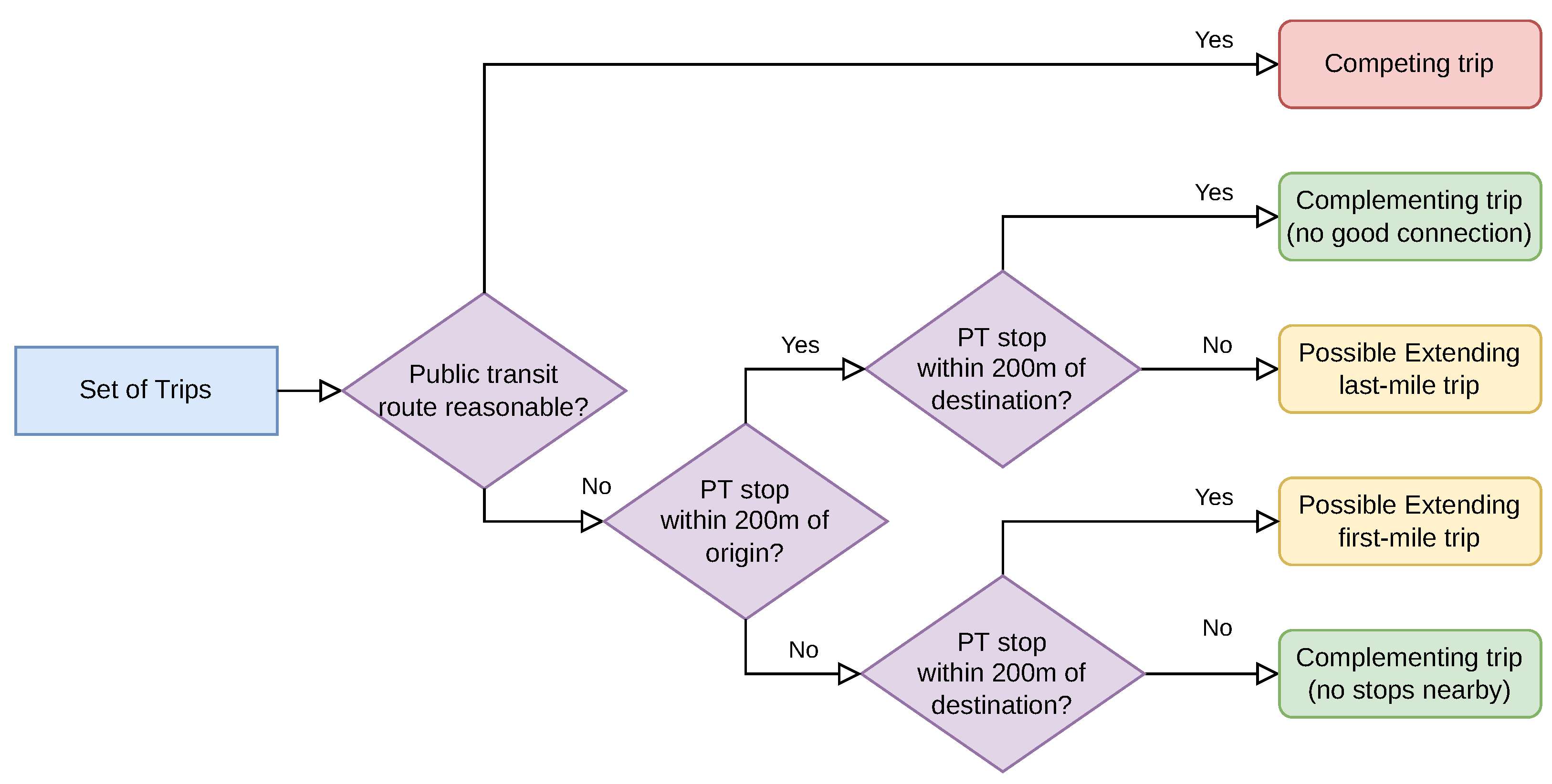
After inferring the trips from the GBFS data stream, we analyze the potential influence of micromobility trips on the public transportation network. For this, we compute the public transportation travel time of the trip with Graphhopper by importing the public transportation schedule in the GTFS format (https://developers.google.com/transit/gtfs/ accessed on 5 March 2022). If no reasonable public transportation trip is found, we compute the walking time for the trip. For the analysis, we assign each customer trip a label with the workflow presented in Figure 3. The label categorizes a trip as a potential competing or complementing trip. A trip may either be complementing because the bus service is currently not in operation or because no public transportation stations were in the vicinity of the origin and destination of the stop. If the trip could also reasonably be undertaken with public transportation, we classify the trip as a competing trip. If the public transit trip was not reasonable, we assume that the public transportation offer in that area or time is not good enough developed, so that micromobility rather complements a non-existing public transportation route. We define a reasonable trip to be a trip, for which the trip time t of the micromobility is not factor f times faster than the fastest public transportation trip. Thus competing is defined as follows: $\mathit{trip} \mathit{is} \mathit{competing}\iff f·t_{\mathrm{micromobility}}\ge t_{\mathrm{public} \mathrm{transit}}$. This means that we define a public transportation trip to be reasonable, if it is not substantially slower than the corresponding micromobility trip. Graphhopper also incorporates possible waiting times at public transportation stops when computing the public transportation trip time. If the trip is not directly classified as a competing trip, we also consider trips extending first- or last-mile trips to/from public transportation stations. The cutoff range for the next public transportation stop is defined as 200 m as it gives a reasonable balance between trips starting or ending near public transportation stations. If a service public transportation stop is at the trip’s origin but not at the trip’s destination, we classify the trip as possible extending first-mile trip. Respectively, if a service stop is nearby the destination of a trip, but not at the origin, we define a trip as a possible extending last-mile trip. Finally, if the trip occurs neither near a public transportation stop nor ends there, we classify the trip as complementing. The complementing and competing labels give a good overview of whether micromobility is used in conjunction with public transportation or instead rather replaces it. The assignment of a potential first-mile or last-mile extending trip instead represents the potential of micromobility in conjunction with public transportation rather than verifying how a trip has been conducted, as we only check whether a trip starts or ends near a public transportation stop.

3.2. Validation of Trip Inference

In this study, we cannot directly compare the list of identified trips with the usage data of the micromobility operators as we do not have any usage data as a ground truth. Reck et al. followed a similar approach to ours for inferring trips from the operator’s API while also having access to real usage data from the operator [7]. They compared the inferred trips with the list of actual bookings (i.e., trips) and reached an accuracy of around $95\%$ on data with a resolution of 1 min with their algorithm. This means that the largest remaining unknown variable for possible inaccuracies in the inference step is the sampling interval of the data. As our study analyzes the data for over a year to identify seasonal trends, we opted for a 10-min resolution for the whole dataset. To analyze the inference algorithm’s validity with a 1-min interval, we assume that, due to the similarity of the algorithms, our implemented trip inference also reaches a comparable accuracy to [7] on a 1-min dataset. To examine the accuracy regarding a 10-min resolution, we captured 1-min data for roughly 3 weeks. With the 1-min dataset as ground truth, we compare its results with the results of the 10-min dataset in the same time to determine the impact of the sampling rate on the trip inference algorithm.

Table 2. Descriptive statistics with a 1-min and 10-min resolution over a timespan of 3 weeks. For the 10-min resolution the deviation to the 1-min resolution is given in percentages.

	One-Min Resolution		Ten-Min Resolution
	E-Scooter	E-Bike	E-Scooter	E-Bike
Total number of trips	44,257	3736	45,935 (3.65%)	3429 (8.22%)
Number of customer trips	34,410	3603	39,761 (15.55%)	3376 (6.3%)
Number of charging trips	4920	0	5384 (9.43%)	0 (0%)
Number of rebalancing trips	4927	133	790 (83.97%)	53 (60.15%)
Mean trip distance	1946 m	3327 m	1721 m (11.56%)	3322 m (0.15%)
Mean trip duration $\Delta t_k$	665 s	960 s	1082 s (62.71%)	1420 s (47.92%)
Mean trip duration $\Delta t_{est}$	418 s	719 s	371 s (11.24%)	718 s (0.14%)
Mean trip duration $\Delta t_{approx}$	606 s	883 s	546 s (9.99%)	888 s (0.57%)
Total fleet size	1878	264	1803 (3.99%)	264 (0%)
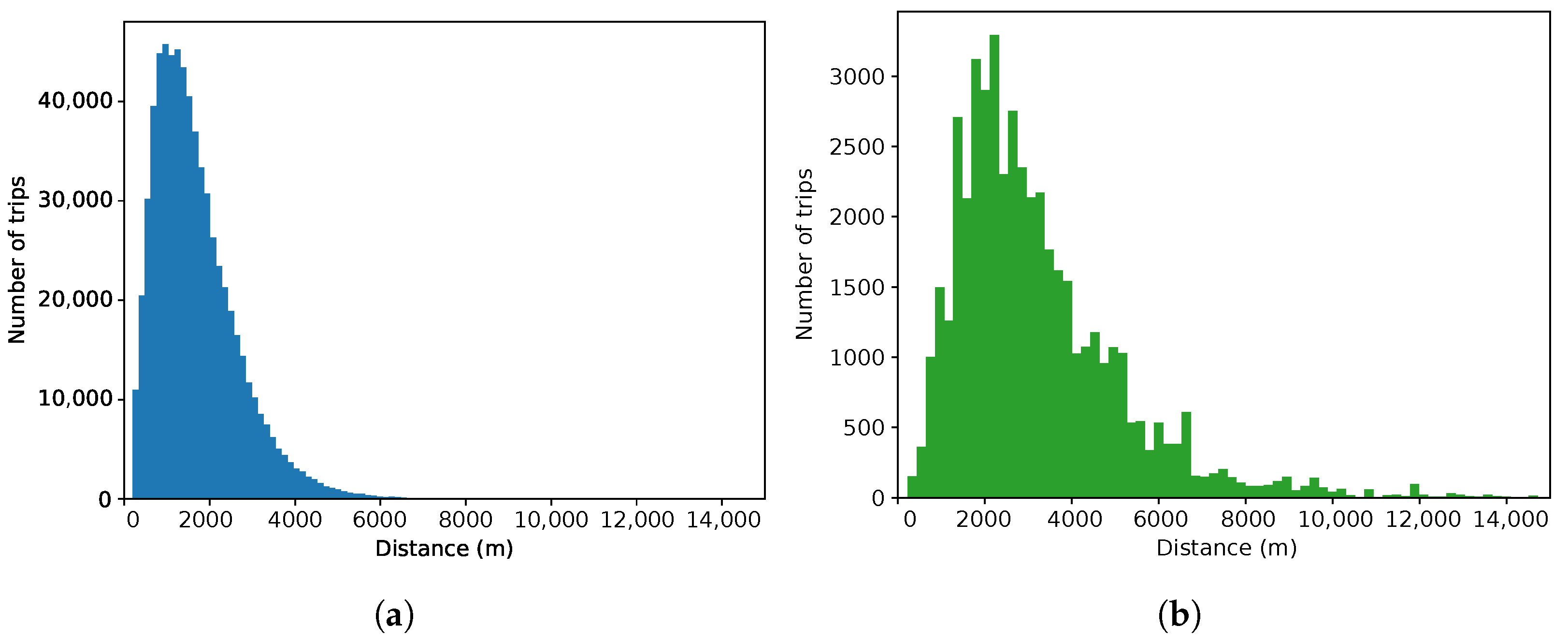
Total used fleet size	1749	258	1757 (0.46%)	257 (0.39%)

shows the descriptive analysis of the 1- and 10-min datasets, and Figure 4 shows a histogram of the number of customer trips plotted against the distance of the trips for both datasets. Table 2 differentiates between different time measurements of the trip. The metric $\Delta t_k$ measures the time by just comparing the logs, thus likely being accurate for the 1-min dataset, but not for the 10-min dataset. $\Delta t_{\mathit{est}}$ is the trip time of the fastest route computed by the routing engine Graphhopper with special e-scooter and e-bike profiles. The travel time $\Delta t_{\mathit{est}}$ was often observed to be too fast when comparing it to $\Delta t_k$ on the 1-min dataset; therefore $\Delta t_{\mathit{approx}}$ approximates the travel time by adding offsets to $\Delta t_{\mathit{est}}$ that incorporate the time required for starting and ending a trip. The travel time approximation $\Delta t_{\mathit{approx}}$ has proven to be the most accurate and most insensitive to different data resolutions; hence we apply this metric for the remainder of the evaluation.

Table 2 shows that overall the number of trips stays similar. However, more e-scooter customer trips have been identified in the 10-min dataset, whereas fewer e-bike customer trips have been identified. The histogram in Figure 4 shows that the inference algorithm more often misclassifies short e-bike customer trips in the low-resolution dataset. With a higher resolution of 1 min, these trips could more likely be identified as false positives. Longer e-scooters trips are more consistently identified in both datasets. For e-bikes, short trips have often been filtered as too fast in the 1-min dataset, whereas the algorithm could more accurately detect them in the 10-min dataset. Additionally, more e-scooter trips are classified as rebalancing in the 1-min dataset. This is most likely due to the higher resolution of the data, as it is more likely to identify trips that were too fast to be driven with the vehicle itself. The algorithm identifies more long customer trips in the low-resolution dataset for e-bikes. This effect may occur when a returned vehicle is instantly rented again, resulting in a non-capture of the availability of the vehicle in the dataset. The algorithm may then misclassify several trips performed with the same vehicle as a single longer trip. This effect is more likely to occur for e-bikes, as the utilization rate of e-bikes is higher due to fewer vehicles being available, i.e., the chance of the same vehicle being rented shortly after being returned is higher.

The mean distance of customer trips in the low-resolution data set is longer for e-scooters and nearly identical for e-bikes. For e-scooters, more short-distance trips are detected in the low-resolution data set, hence shortening the mean distance. For e-bikes, the mean distance is nearly identical; hence, the previously discussed distinct effects for identifying fewer short trips and more long trips in the low-resolution dataset seem to cancel each other regarding the average. Table 2 shows that the value of $\Delta t_k$ strongly differs between both datasets. Unsurprisingly, the low-resolution data set has much longer trip durations. A trip can only be intervals of 10 min long, whereas the high-resolution data set has a better approximation of the trip duration based on the inference. To compensate for this significant difference in the duration, we compute an estimated trip duration $\Delta t_{\mathit{est}}$ with a routing engine utilizing OpenStreetMap data. The time $\Delta t_{\mathit{est}}$ is the duration of the fastest route between the origin and destination. With this metric, the trip duration between the 1- and 10-min datasets are much closer to each other again. In practice, the computed trip distance with the routing engine did not capture the duration in which the scooter was in use. This becomes apparent when looking at $\Delta t_k$ for the 1-min resolution and $\Delta t_{\mathit{est}}$, where $\Delta t_{\mathit{est}}$ is much lower. One hypothesis is that the user requires some time for starting and ending the trip, as such $\Delta t_{\mathit{approx}}$ compensates for this with its offset. $\Delta t_k$ is therefore inaccurate for a low resolution, whereas it is highly accurate for high-resolution data. Overall, $\Delta t_{\mathit{approx}}$ works well on both low- and high-resolution data. The fleet size of all providers is nearly identical, where slightly more vehicles have been observed in the high-resolution data set. This difference can most likely be attributed to vehicles for which information has only been published for a brief duration. Zhao et al. [32] summarizes that the sampling rate of the data does not significantly influence the spatial and temporal properties of the trips if it is not larger than 10 min. We agree with the conclusion, as for most tasks, a 10-min resolution of the data is already reasonable, particularly when compensating for the occurring effects with external data such as OpenStreetMap as for most metrics the error is less than $10\%$ after adjusting for inaccuracies. However, specific patterns in the data are missed in our implementation with a low resolution, especially when trips are short and a high utilization of vehicles is reached. Then the classification of trips suffers, whereas the total number of inferred trips stays similar. Hence, a higher resolution should be preferred for specific tasks or when an exceptionally high data accuracy is necessary. For a general understanding of the usage characteristics a resolution of 10 min is accurate enough and shows that the inference step reliably transforms the operator’s data into a list of trips.

4. Analysis of the Aachen Case Study

The analysis covers the supply-side (operator view) and demand-side (traveler’s view) analysis of the data. For the supply-side view, we analyze the micromobility operator’s fleet and the distribution of vehicles in the service area. The demand-side study features both a spatial, temporal, and spatio-temporal analysis. For this, we analyze temporal patterns in the usage characteristics over a year. Furthermore, we examine the starting points and endpoints of trips in terms of land use to elicit possible trip purposes. Lastly, we compare the demand for micromobility to the supply of public transportation to understand how micromobility interacts with public transportation.

4.1. Results

Table 3. Descriptive statistics for the micromobility supply and demand in Aachen in a year with aggregated mean values.

	E-Scooters	E-Bikes
Total number of customer trips	664,614	47,040
Total number of charging trips	115,356	0
Total number of rebalancing trips	13,383	936
Total number of deploying trips	2495	106
Mean trip distance	1680 m	3219 m
Mean trip duration $\Delta t_{approx}$	534 s	865 s
Mean available fleet size	1163	213
Total number of vehicles observed	3931	289
Total number of vehicles observed with swappable battery	2650	0

shows the overview of the inferred trips from December 2020 to December 2021. The largest number of identified trips are customer trips for e-scooters and e-bikes. For the docked e-bike-sharing system no charging trips have been detected as they are automatically charged upon docking, whereas e-scooters have regularly been manually charged. E-scooters have a higher number of rebalancing trips, most likely as their location is not determined by a location of a dock but only by a geofence. Overall, the fleet of e-scooters is much larger than the e-bike fleet, thus also decreasing the mean vehicle utilization rate.

In

Table 4. Descriptive operational statistics for an average vehicle in Aachen in a year.

	E-Scooters	E-Bikes
Average service days per vehicle	131.13 days	314.94 days
Average number of trips per vehicle	155	155
Aggregated trip distance per vehicle	261.34 km	497.80 km
Aggregated trip duration $\Delta t_{approx}$ per vehicle	23.07 h	37.02 h

, the average data per device is shown. The table shows that e-scooters have a more limited usage duration than e-bikes. E-scooters are in operation for roughly 131 days, whereas e-bikes are in service for 314 days, i.e., nearly the complete observation period. When regarding the number of observed vehicles in Table 3, we can see that a much larger number of vehicles have been observed for e-scooters. This means that either e-scooters are being replaced after 131 days in average, that the providers change the IDs of the vehicles, or that the vehicles are swapped with vehicles in other cities, outside of our data. Interestingly, due to the larger number of trips performed with e-scooters in total, the number of trips per vehicle is comparable between e-bikes and e-scooters, even though the e-scooter fleet is much larger. On average, the distance driven with each e-bike is nearly twice as considerable as for e-scooters. In contrast, the total operating time per vehicle is around 10 h longer. These results agree with other studies’ results that e-bikes are often used for longer trips than are e-scooters. Furthermore, e-scooters are more often used, possibly due to their ubiquitous availability, resulting in higher flexibility. The mean number of utilized vehicles is higher for e-bikes, most likely because fewer vehicles are available, thus increasing the utilization. Even on the days with the highest vehicle utilization, not all vehicles have been used for trips, possibly hinting at a potential for optimization by reducing the micromobility fleet.

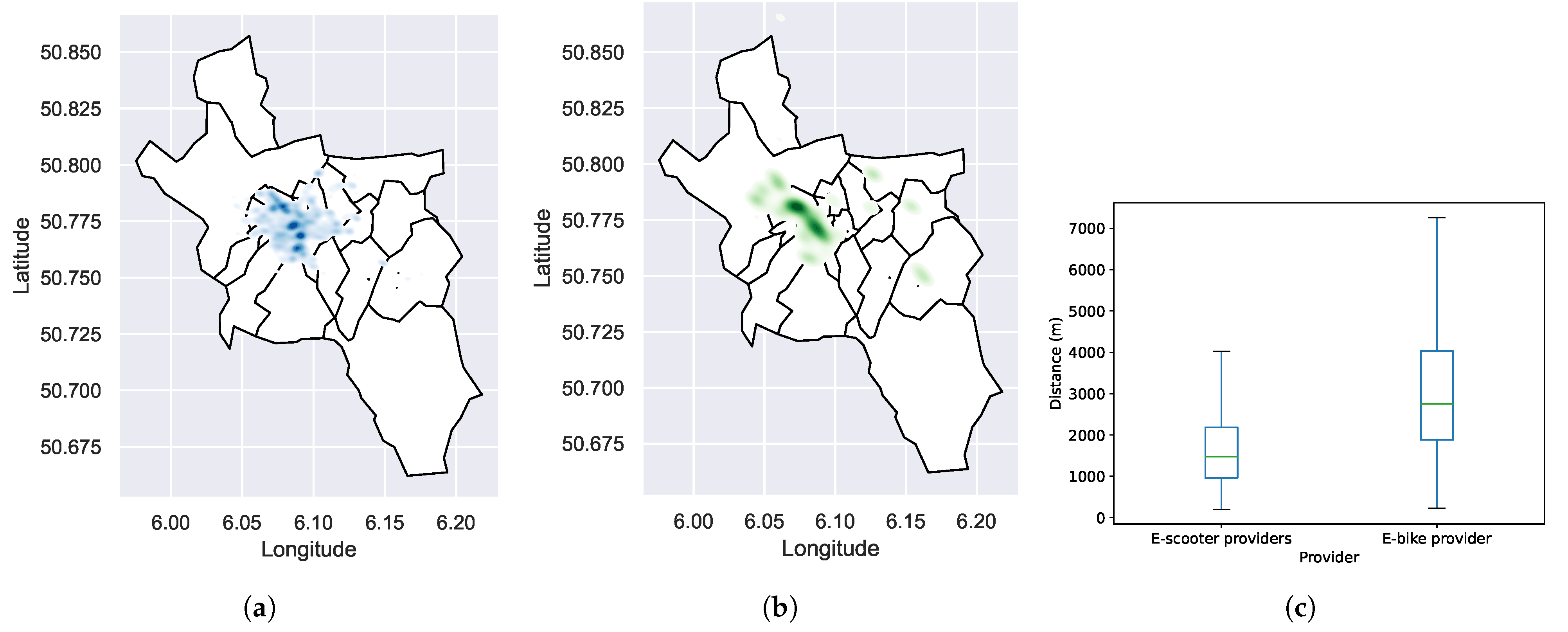
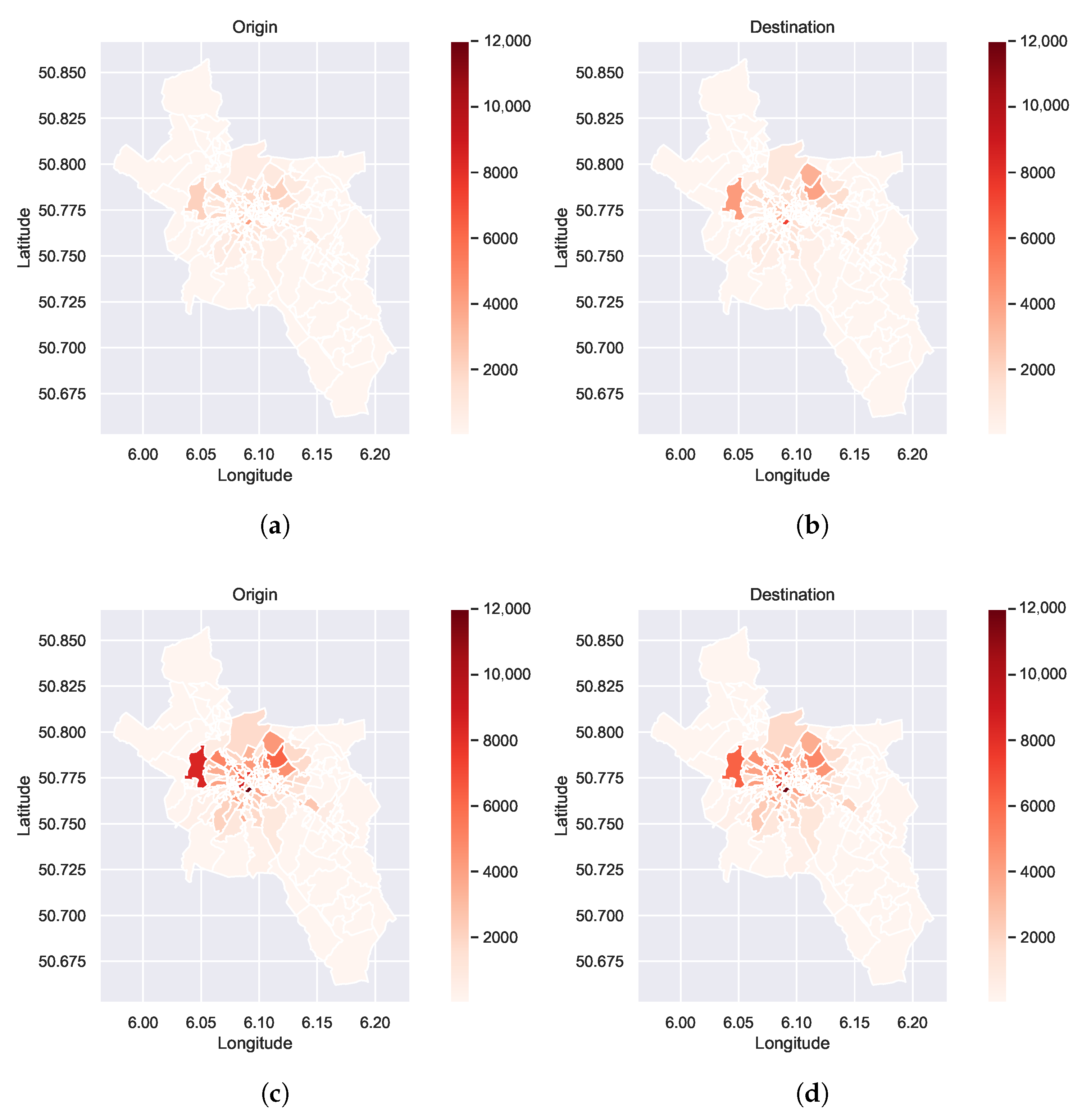
After the overview over the fleet size of the different providers, the aggregated distribution of the vehicles in the city is shown in Figure 5. The supply of available vehicles forms multiple hotspots in the city. The three main hotspots occurring are around the general city center, particular buildings of the university campus in the West, and Aachen central station in the South. This agrees with previous research that micromobility usage is especially high in the city center and near areas of the university campus. Interestingly, the hotspots for e-scooters and e-bikes are different. The results indicate that e-bikes are used for different types of trips than are e-scooters or that different patterns of hotspots are induced due to the location of the e-bike docks. For e-bikes, the hotspots are more dense and the spread in the locations is narrower, most likely due to the station-based concept. For e-scooters, the distribution in the city is more even. The distribution of e-scooters and e-bikes matches the service area or bike-sharing station locations shown in Figure 2a.

Figure 5c shows a boxplot of the distance of e-scooter and e-bike trips. The figure confirms the results of related work that e-bike trips are substantially longer, whereas e-scooters are primarily utilized for trips shorter than 2 km. E-bikes are still often used for trips with a distance of 4 km. The distribution of different distances is also plotted in Figure 6. For e-scooters, the graph ascends quite fast and forms a strong slope with a maximum at around 2 km. Nearly no trips with a distance longer than 6 km are performed. On the other hand, e-bikes have their peak at around 3 km. Afterward, the distances do not descend as abruptly, with longer distances, as e-scooters, meaning that e-bikes are regularly used for longer trips. The e-bike data also shows more irregular spikes in the distances than the e-scooter data shows. This effect may hint at the station-based nature of the e-bike service, meaning that popular routes between stations yield specific distances, explaining the discrete-looking spikes in the graph.

4.1.1. Spatial

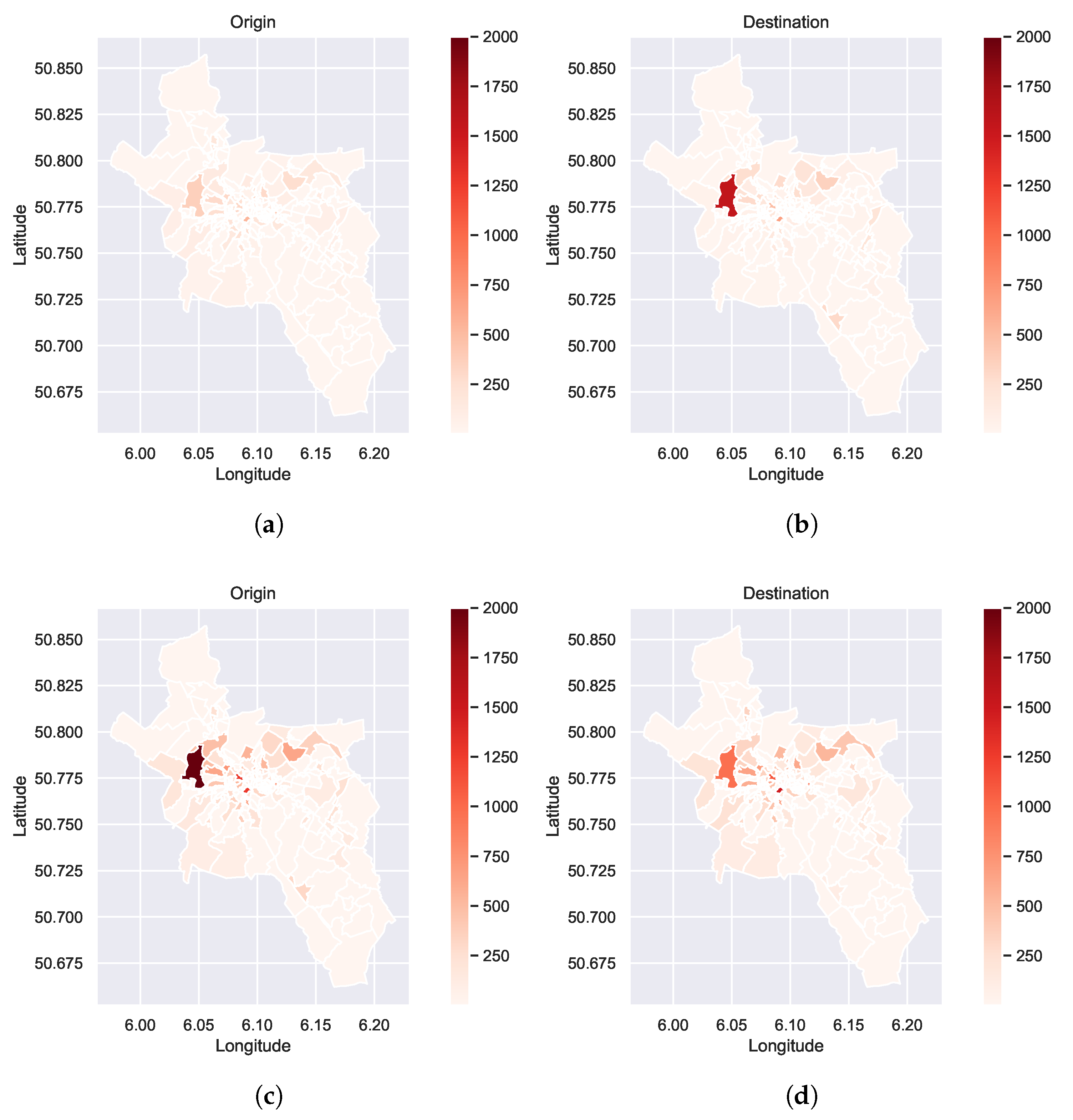
After analyzing the general features of micromobility trips in Aachen, we move to the spatial analysis. Here, we focus on the origin and destination of trips and on the feature of these areas. Figure 7 shows the number of e-bike trips starting and ending of trips in specific zones in Aachen in the morning (05:00–12:00) and in the afternoon (12:00–09:00) over the whole analysis period. Analogously, Figure 8 shows the trip’s origin and destination in the morning and afternoon for shared e-scooter traffic. We start with the number of e-bike trips as certain patterns are more visible.

In the morning, most e-bike trips originate near Aachen central station, a geographically small area in the south of the city center. The smaller hotspots in the middle correspond to areas near the city center. The hotspot in the west is an active part of the university campus hosting a large university hospital and a large university dormitory. Interestingly, when looking at the destination of the trips in the morning, they primarily target the large campus and university hospital area. All other locations are significantly less likely to be the destination of a trip. Even the central station is not a popular destination, meaning that more people use e-bikes to travel from the train station to their destination than people use them to reach the central station. It is clear that the university campus area to the west has a large inflow effect for e-bike journeys.

In the afternoon, the observed pattern, interestingly, mainly flips. Most trips start near the university campus area to the west. In the afternoon other areas such as the city center and the central station are also likely origins for trips. The destinations of most trips is the central station, the city center area, and also the campus area. The substantial trips to the central station could be attributed to commuters returning to the central station. Overall, the destinations are more evenly spread over the whole city. The patterns in the morning and in the afternoon indicate that e-bikes are often used for commuting in Aachen as many travelers travel from the central station and various other areas mostly to the campus and the university hospital region. This area features many employment opportunities and is also an important area for students. In the afternoon, many trips originate there, going back to the central station and various other regions, which may indicate that travelers return to their home locations. The larger spread in origins and destinations over the city in the afternoon could be attributed to more recreational trips occurring in the afternoon than in the morning.

For e-scooters, the observations in Figure 8 differ from the spatial results for e-bike use. Although the most frequently traveled e-bike districts are also one of the most traveled e-scooter districts (Aachen central station and large university campus), the journeys are additionally more evenly spread out in the city. This can be seen especially well in Figure 7b and Figure 8b. The hotspots of the trip destination of e-bikes and e-scooters are very similar, but the hotspots are more focused for e-bikes. One explanation would be the location of the e-bike stations, i.e., only certain districts have an e-bike station, causing the demand to be focused on these districts. When looking at the distribution in Figure 2a, it can be seen that the stations themselves are also located in nearly all districts; thus the difference between the usage is more likely due to different usage characteristics of the services. In general, the analysis show that e-scooter usage of origins and destinations does not differ that much with time, and the most important areas for trip origins and destinations in Aachen are the central station, the large area of the university campus, and the city center. In contrast to e-bike trips, e-scooter trips are fairly balanced with the most popular trip origins also being popular trip destinations for both the morning and afternoon. In summary, the results indicate that e-scooter usage is more spread out with a smaller focus on certain areas than e-bikes.

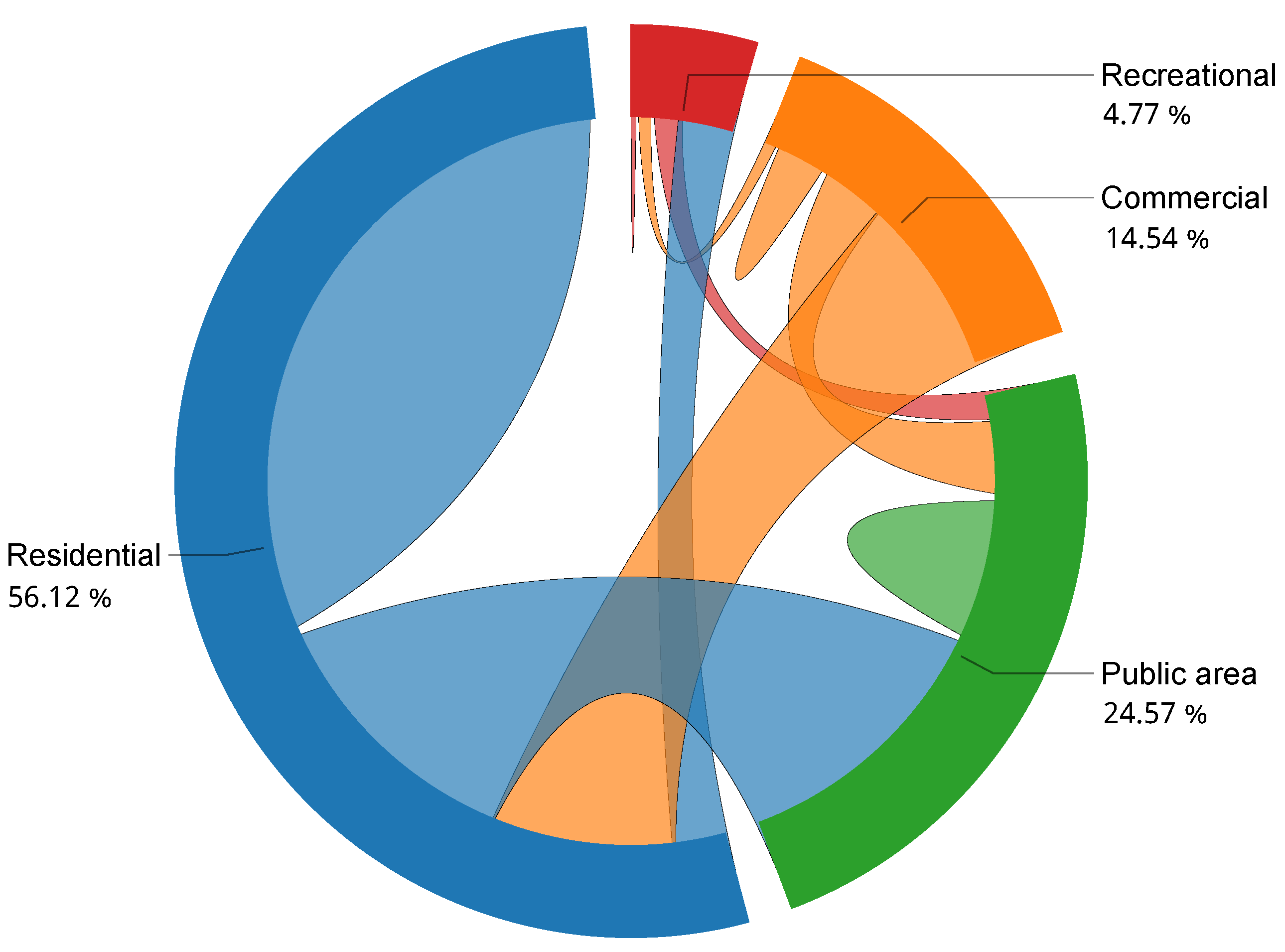
Next, land use for trip origins and destinations has been analyzed by using the land use data from OpenStreetMap with an Overpass server. Under the assumption that the inferred trip’s origin and destination is correct, the land-use assignment corresponds to a simple look-up of the land-use type in the OpenStreetMap data. This means that the analysis is as accurate as the data in OpenStreetMap. The analysis differentiates between the different land use types of residential, recreational, commercial and public areas, similar to [8]. For this, we have also grouped the detailed land use data obtained from OpenStreetMap into coarser buckets of land use in order to visualize this data.

Table 5. Land-use statistics and respective e-scooter and e-bike trips starting and ending in those areas.

Land Use Type	Area		Trip Share		Land Use Filter
	Total	Percent	Origin	Dest.
Residential	$14.52$${\mathrm{km}}^2$	$64.90\%$	$56.12\%$	$56.35\%$	Residential Buildings and Garages
Commercial	$2.462$${\mathrm{km}}^2$	$11.00\%$	$14.54\%$	$14.99\%$	Commercial, Industrial, and Retail
Recreational	$0.924$${\mathrm{km}}^2$	$4.13\%$	$4.77\%$	$4.73\%$	Allotments, Parks, Forests, Meadow, Greenfield, Flowerbed, Religious, Village Green
Public Area	$4.465$${\mathrm{km}}^2$	$19.95\%$	$24.57\%$	$23.93\%$	Brownfield, Cemetery, Construction, Railway, Road, Civic, Grass, Farmland, Farmyard

shows the raw data and Figure 9 shows a chord diagram visualizing the trips between different land use types. The arcs inside the chord diagram visualize the number of trips with a specific land use type at the origin of the trip. The width of the arrows between the arcs visualize how many trips have certain land use destinations. The residential and the public areas are the largest trip origins and destinations. These land use types are also consistently the largest areas in the observed area of Aachen. When analyzing whether certain areas are more often the origin or destination of a micromobility trip related to their size, we did not find many hints that certain areas are favored. Overall, the size of the area strongly correlates to the fraction of trips originating from this land use type. This indicates that micromobility vehicles are used for all kinds of activities and that their usage is not restricted to certain activities such as commuting, as the land use area percentage is similar to the trip share. Commercial and public areas are slightly underrepresented when compared to residential areas; however, this can largely be attributed to where scooters are parked after a trip, making it more uncommon to directly park an e-scooter in a commercial area, rather than a nearby road, which may already belong to the residential area again. For policy-makers this means that micromobility may not be restricted to a single use-case but rather micromobility users use this transportation mode for all kinds of purposes. As such, it may be difficult for policy-makers to directly target micromobility users with new regulations. In summary, this indicates that e-scooters and e-bikes are used for all kind of trips from a land-use analysis. Nevertheless, the previous temporal and spatial analysis remains valid when it shows that, regarding micromobility trips in more detail with contextual knowledge of the spatial properties in Aachen, certain characteristics are extractable that are missed when regarding the land-use type. This result highlights the need to manually analyze the trip data in-depth as otherwise correlations might be missed.

4.1.2. Temporal

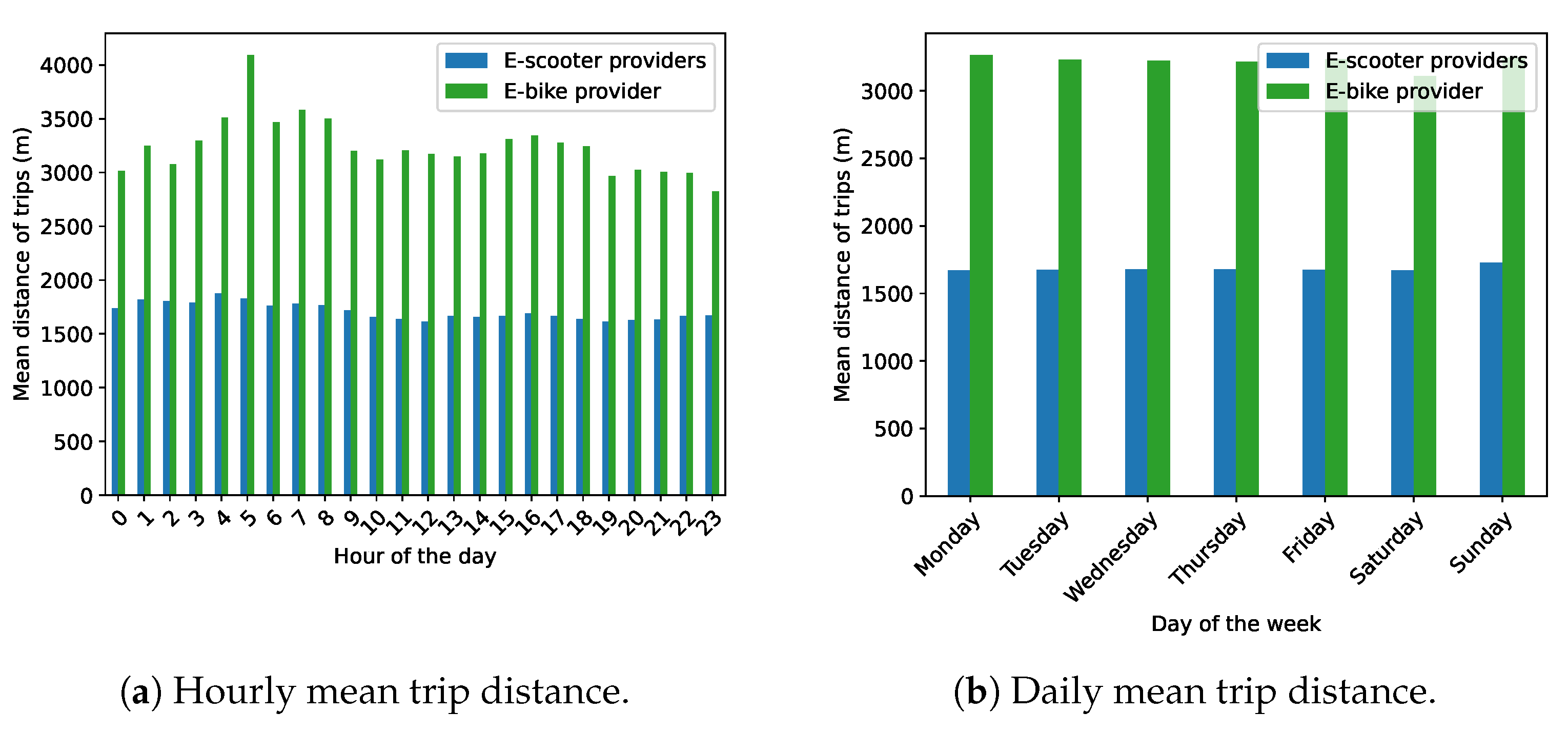
As a next step, we investigate the temporal characteristics of micromobility usage. Figure 10 shows the distance of trips during a day and a week. The figures show that there is no considerable variation in the distance of trips for different times. Slight variances in trip length exist for interday time differences, whereas intraday variations are barely noticeable. E-scooter trips show even less variation, whereas e-bike trips have a minor increase in distance in the early morning hours. This may indicate longer trips may be performed when commuting to the workplace, however, a similar peak cannot be seen in the afternoon.

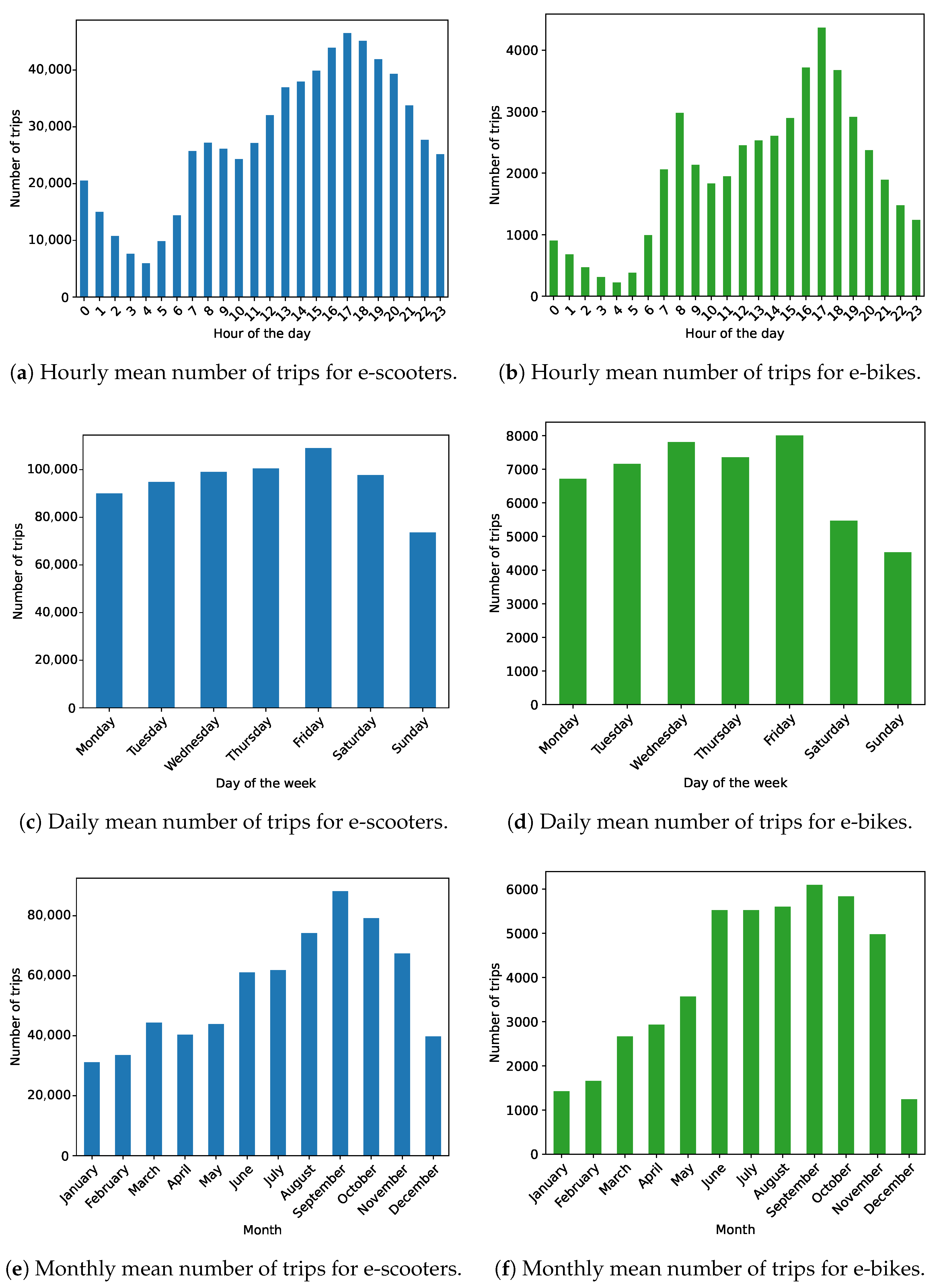
Figure 11 shows the aggregated hourly, weekly, or monthly mean number of trips. The peak of micromobility usage is often reached in the late afternoon and early evening hours from 16:00 to 18:00. In contrast, the least micromobility is used in the early morning from 03:00 to 05:00 (see Figure 11a,b). E-bike usage also shows a significant peak at 08:00 in the morning and at 17:00 in the afternoon, hinting at the possibility of commuting to and from work as this pattern matches a typical commuting pattern. These peaks also exists for e-scooters, but are not as distinct as for e-bikes and are more spread out. E-scooters are most often used in the late afternoon until late in the evening, indicating that e-scooters may more often be used for recreational trips. The number of e-bike trips already declines much earlier in the day, bu e-scooter usage is still quite high in the very late-night hours and very early morning hours.

When looking at the number of trips aggregated to days in a week in Figure 11c,d, one can observe that e-scooters are most often used on Friday and Saturday. The large usage of e-scooters on Saturday supports the hypothesis that many e-scooter trips are for recreational purposes. The lowest usage of e-scooters is recorded on Sundays. Docked e-bikes, on the other hand, are primarily used during the week and the least on Saturday and Sunday. In particular, the drop on Saturday is very distinct for e-bikes, further indicating their commuting purpose. We can identify no clear trend for the remaining days, and the variations in the number of trips do not show a clear pattern.

The aggregation to periods of months shown in Figure 11e,f is given mainly for completeness. During the data gathering, there was a soft lockdown in Germany due to the COVID-19 pandemic from April 2021 to June 2021 with a nightly curfew; even before that, local lockdowns and restrictions strongly influenced the mobility behavior. These lockdowns can also be seen in the data. The number of trips strongly rises in June 2021, most prominently shown in the e-bike data. However, the data may slightly hint at a lower micromobility usage in the winter months (e.g., in November 2021), probably due to more precipitation, as shown by [21]. In further research, we hope to obtain data that are not influenced so strongly by external factors such as travel restrictions.

4.1.3. Impact on Public Transportation

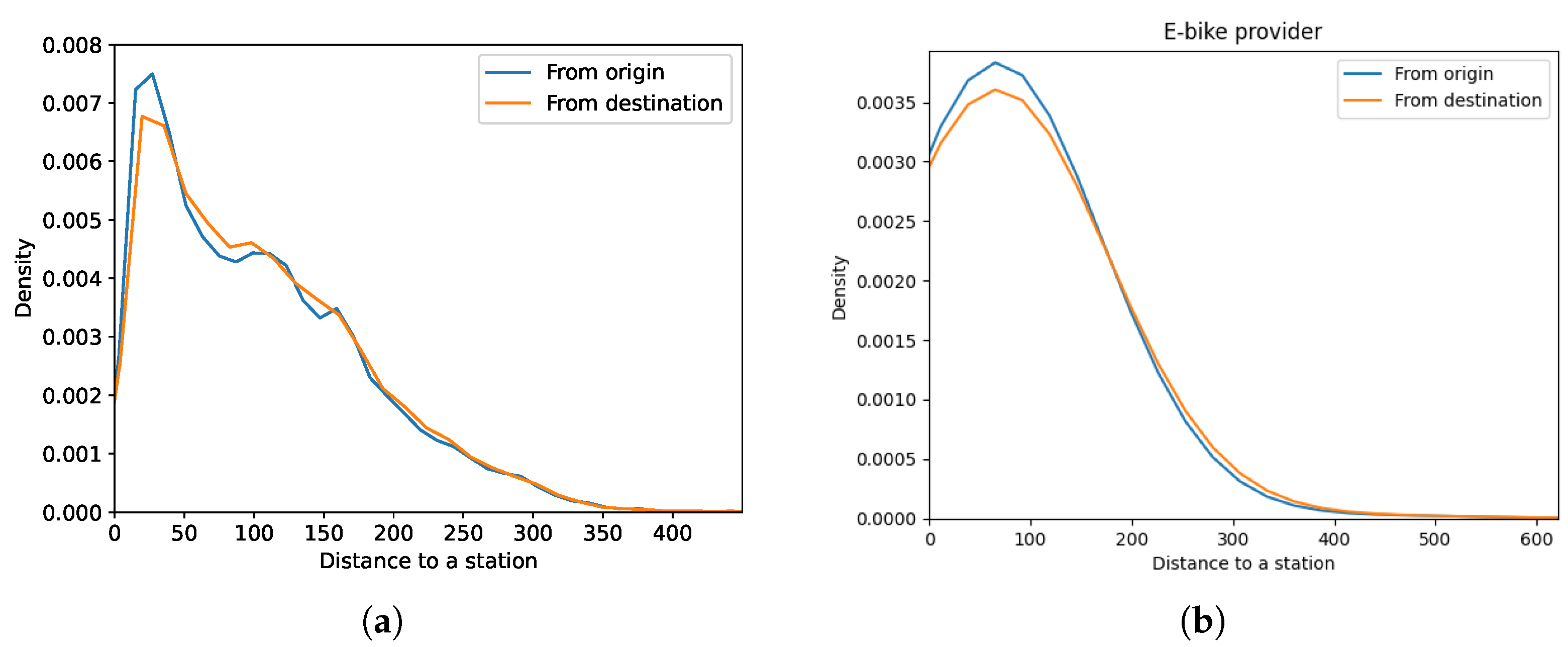
As a final step of the analysis, we analyzed the interactions between micromobility trips and the existing public transportation. For this, we followed the workflow as described in Figure 3, i.e., for all inferred micromobility trips, we computed how long this trip would have taken with public transportation, taking into account the locations of public transport stops and its fixed schedule. Figure 12 shows the distances of origins and destinations to public transportation stops. It shows that for both e-bikes and e-scooters the nearest public transportation station is most often not further away than 350 m to the origin or the destination of the micromobility trips. In Aachen, most of the micromobility usage is observed in the central areas of Aachen, where a significant density of public transportation stops exists, explaining the proximity to public transportation stops. However, in a public transportation network, being near a stop does not necessarily mean that there exists a good connection to the destination. The figure shows that users most likely do not prefer micromobility over public transportation because of missing public transportation stops, as the next bus stop is not always far away. We hypothesize that users are more likely to perform a trip with micromobility in areas or times where public transportation is not as accessible, thus increasing the time required for users to perform the trip.

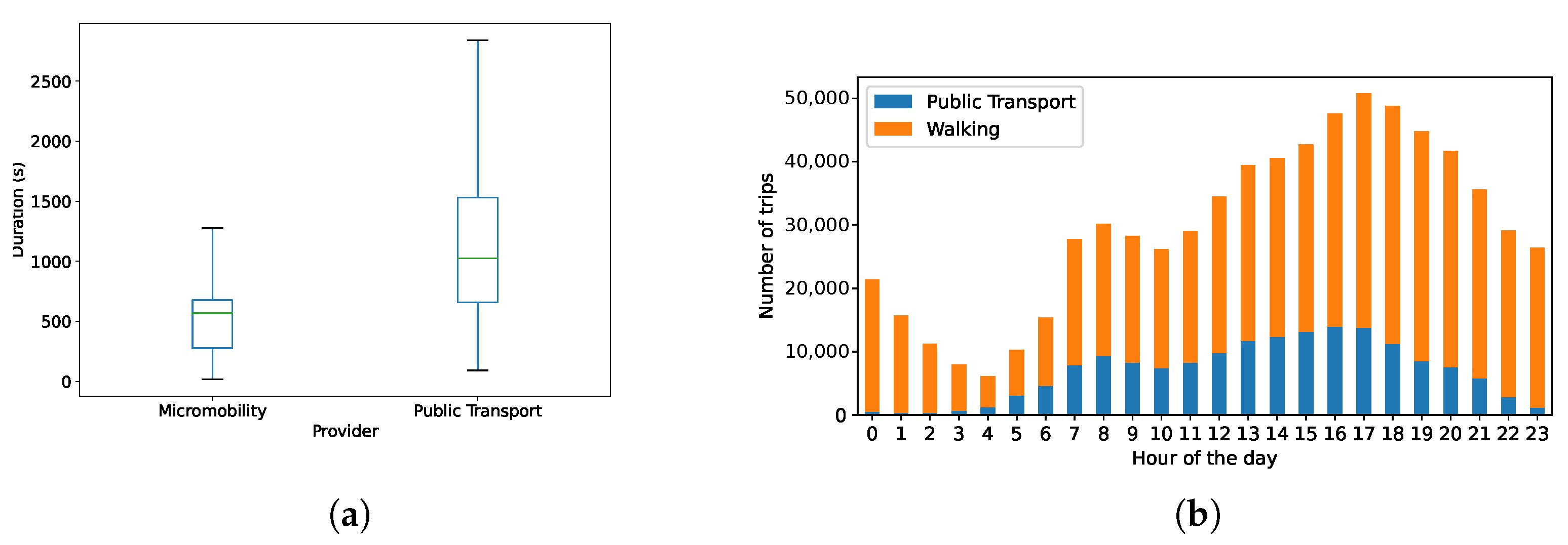
For further investigation, we have also regarded the time it would have taken to travel from the origin to the destination of all trips via public transportation or walking if no bus is reasonably available. The time for taking public transportation is therefore defined as the minimum of the time using public transportation or walking the entire length of the trip. Figure 13a shows a boxplot of the time of trips for micromobility and assumed public transportation trips, whereas Figure 13b shows a distribution of assumed public transportation trips over hour per day, categorized by whether walking or public transportation is faster. The boxplot shows that micromobility journeys are substantially faster than the assumed public transit journeys for the same trips. This is due to the fact that public transit journeys also take into account the walk to the nearest stop, the wait for the vehicle, and the taking of the vehicle, the potential transfer to other vehicles, and the walk from the final stop to the trip’s destination. Figure 13b shows that for a substantial number of trips, it is actually faster to walk the entire trip length than to take public transportation. In particular, at night, when public transportation is unavailable, the number of trips for which is faster to walk strongly rises. This indicates that micromobility complements public transportation as for many micromobility trips, and it is even faster to walk the trip than to take public transportation; hence public transportation is likely not seen as a viable alternative.

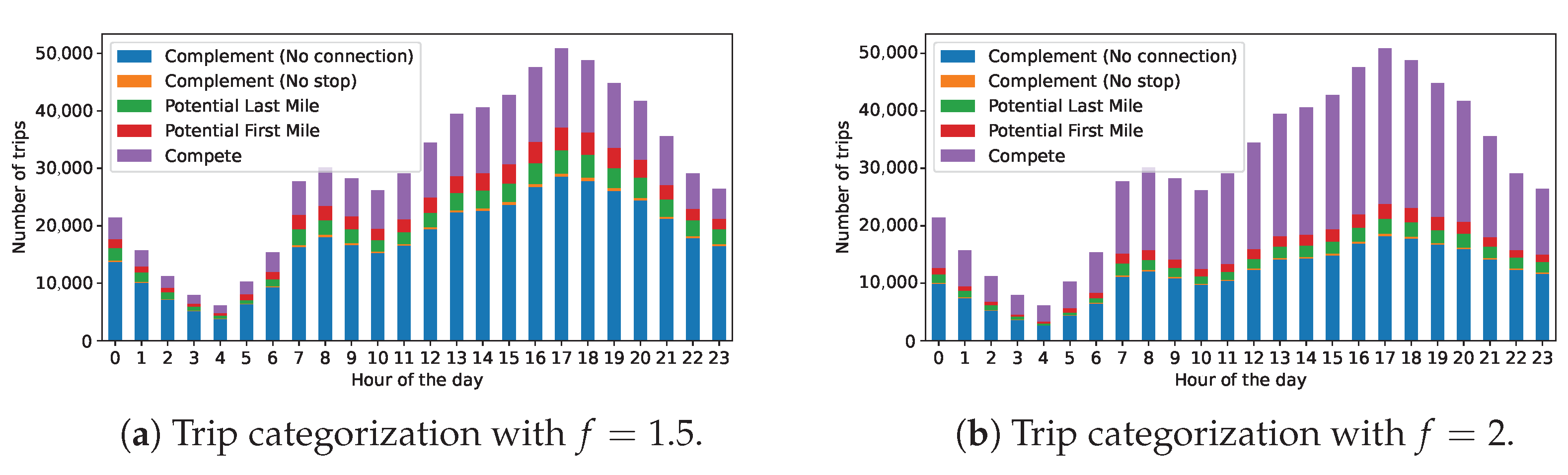
Next, for quantifying which trips might be complementing or competing with public transportation, we categorized trips based on the difference in duration between micromobility trip and public transportation trips.

Table 6. Comparison of customer trips based on their relation to public transport. The factor f defines how much faster a micromobility trip must be compared to the respective public transportation in order for the trip to be classified as complementing. This means that the factor f defines the reasonability of the public transportation route.

f	Mode	Compete	Extend (First- or Last-Leg)	Complement (Stop)	Complement (Connection)
1.5	E-scooters	165,447 (24.90%)	111,919 (16.85%)	7834 (1.18%)	379,338 (57.08%)
	E-bikes	8806 (18.72%)	774 (1.65%)	925 (1.96%)	36,533 (77.66%)
2.0	E-scooters	334,501 (50.48%)	74,003 (11.14%)	5386 (0.81%)	249,648 (37.57%)
	E-bikes	21,415 (45.53%)	659 (1.40%)	745 (1.58%)	24,219 (51.49%)
3.0	E-scooters	569,447 (85.70%)	21,569 (3.25%)	1579 (0.23%)	71,943 (10.82%)
	E-bikes	41,016 (87.20%)	308 (0.65%)	41 (0.09%)	5673 (12.06%)

shows the classified trips in Aachen for different factors f indicating how much faster a micromobility trip must be before being categorized as complementing public transportation. Here, the key idea is that people accept that the public transportation trip takes longer, but if it takes substantially longer, it is no longer seen as a reasonable alternative. We have tested the competition between micromobility for factors f of $1.5,2,$ and 3. A factor of 2 means that a micromobility trip is assumed to be competing, if it takes less than twice the time of the respective public transportation trip from the same origin to the same destination. The results indicate for a lower threshold of accepting slower public transportation as an alternative, many micromobility trips are complementing public transportation. When increasing the factor f, the number of competing trips sharply rises. At the same time, the table also highlights that micromobility complements public transportation by offering their service mostly in times when public transportation is not an option, i.e., compare number of complementing trips for $f=3$. Here, micromobility trips are already competing with the walking trips when no public transport route is available and the only complementing trips are trips that are very long. It is unclear which factor f best represents the mode choice for people, i.e., starting with which factor people will prefer micromobility over public transportation or walking. Furthermore, the results confirm that most often the distance to the next public transportation station is not the problem, but the connection between different bus lines with transfers. This can be seen by the low number of complementing trips occurring due to no stop point being present and the distance of public transport stops to trip origins and destinations in Figure 12. Micromobility has the advantage of being usable door-to-door and that no transfers are necessary, thus strongly reducing the time required for certain routes in comparison to public transportation. Under the assumption that people accept public transportation as an alternative if it is not less than half as fast as a corresponding micromobility trip with $f=2$, around $50\%$ of e-scooter trips are competing and another $40\%$ of trips are complementing public transportation. When setting the factor to 3, primarily long trips in the night when the bus service is not operating at all are marked as complementing trips, whereas during the day most trips are marked as competing.

Figure 14 shows the number of complementing, competing, and extending trips per hour of the day depending on whether $f=1.5$ or $f=2$. Here, we can see that during the day the relative number of competing trips is higher than in the night where public transportation is unavailable. When comparing the figure with Figure 13b it becomes apparent that the number of competing trips rises with the number of trips that are feasible with public transportation. Most of the complementing trips are faster not because the public transportation system is unavailable in the night hours or because the next public transportation stop is too far away, but because the public transportation route between the trip’s origin and destination takes too long, possibly because of the wait for the vehicles and the transfer to other vehicles. The figures show that in Aachen, micromobility trips are often not replacing public transportation, but complement them by offering a service that serves origins and destinations that are not well connected by public transportation.

The overall results indicate that e-scooter and e-bike trips are often started or ended near public transportation stops as the public transportation network is dense in the service area. For e-bikes, the first- and last-mile extension is much lower, because most bike-sharing stations are built next to public transportation stations, which means that our algorithm does not flag these trips as public transit extension, as both origin and destination are nearly always near public transportation stops. For e-scooters, the number of competing trips is larger than for e-bikes. The main reason for this may lie in the origin and destination of trips. E-bikes are used relatively often for the trip from Aachen central station to the university campus area, for which no good public transportation route exists, thereby lowering the number of e-bike competing trips. E-scooters, on the other hand, are often rented because of their flexibility, possibly indicating that e-scooters are more often used even though there is a viable public transportation route. In practice, the time required for the trip is not the only factor influencing mode choice, but the results show how much faster micromobility can be in comparison to public transportation. In summary, the results indicate that micromobility trips can replace public transportation trips, but are mostly complementing public transportation services when the service is not operating or not well developed.

4.2. Discussion

The study shows the feasibility of reconstructing trips from the vehicle availability data from the operator enriched with information from openly available geography data and public transportation schedules. In this study, we examined the difference in usage characteristics between dockless e-scooters and docked e-bikes and their potential influence to the existing public transportation network. The results of this study regarding e-scooter and e-bike trips mostly agree with the results of previous studies, confirming the viability of the approach of gathering vehicle locations and inferring the relevant trips. E-bikes are often favored for longer trips when compared with e-scooter usage, possibly due to their higher comfort. E-scooters, on the other hand, are the preferred mode of travel for shorter journeys, possibly due to their high availability and flexibility. In the literature, the primary purpose of e-scooter and e-bike trips are still an ongoing research topic. This study found evidence for a stronger commuting purpose for e-bikes and a larger recreational role for e-scooters; however, further research is necessary. Our results also show especially high micromobility usage in the city center, near the university campus, and near the central station area, agreeing with previous studies. With spatial trip data such as this, the authorities could improve the routes for e-scooters and e-bikes between the most traveled origins and destinations to increase the safety of the transportation mode. The land use analysis has shown that micromobility trips serve all kinds of purposes as the fraction of trips starting or ending in most land use regions equals its relative size.

This study is also one of the first studies to research the connection between micromobility and public transportation with data-driven methods. The role of micromobility together with public transportation is still ambivalent. Although micromobility complements public transportation in times of non-operating or not well-developed areas, some trips also seem to replace public transportation trips. This could indicate that people favor the flexibility and speed of micromobility over public transportation or walking trips, even if viable alternatives are available. These results are especially surprising as all students at the university, the primary usage group of micromobility according to other studies, have free access to public transportation in Aachen, possibly indicating that the trip’s cost is not the primary concern of micromobility users. E-bikes have a higher ratio of trips that have been identified as complementary, agreeing with previous studies that bike-sharing systems can improve the number of possibly commuting multimodal trips. In summary, micromobility definitely complements public transportation in areas and times where it is not an alternative, or when the available public transportation schedules do not connect the origin with the destination in a satisfactory manner. The reason for complementing is nearly always because of the connection between the origin and destination and not because of the absence of public transportation stops. At the same time, however, micromobility also replaces some viable public transportation trips.

The results show that further research is necessary to find regulations that establish micromobility as a service next to public transportation that complements its usage rather than competing with it. When regarding the complementary trips of micromobility, it becomes evident that the public transportation network is fairly inaccessible in certain areas, even when vehicles are operating (Figure 13b). When adapting the public transportation network, these areas are of particular interest, because there micromobility is much faster than public transportation for most routes. Hence, one reason for people choosing micromobility over public transportation or an intermodal trip is likely the shorter duration of the door-to-door micromobility journey as no transfers are necessary. This choice is particularly noteworthy here, as the primary user group of micromobility identified in other studies is comprised of students near the campus area, which have free access to public transportation in Aachen. Therefore, policymakers and transportation planners should expand the public transportation service so that more routes are adequately served. Furthermore, the advantages of each transportation mode should be exploited as well as possible, meaning that the switch between different modes must be simplified. One proposal from the literature is the creation of so-called mobility hubs, where all kinds of mobility services are offered, increasing the feasibility of easily transferring between modes. In the case that mobility operators create such mobility hubs in Aachen at suitable locations, they may promote the usage of micromobility for the first- and last-mile while fostering the use of public transportation between well-connected mobility hubs. In further research, we want to determine the impact of the mobility in Aachen when creating mobility hubs at certain key locations by simulating the potential passenger flow.

5. Conclusions and Future Work

The offer of micromobility services has strongly risen in the past years in urban areas worldwide. The impact of this development and micromobility usage characteristics have often only been researched in cities in the United States of America on data directly offered by the provider due to the legislation in certain cities. Unfortunately, such trip-oriented data is often not readily available in other parts of the world. Therefore, we present an algorithm to infer trips from the availability data providers share with their API to offer their services through their application. We examined the temporal and spatial properties of e-scooter usage with the inferred trips, focusing on the interaction between public transportation and micromobility.

To the best of our knowledge, this study analyzes the most extensive dataset of high-quality self-inferred trips up to date. Compared to the publicly available datasets, the set of inferred trips offers a larger spatial and sometimes also a temporal resolution. For temporal factors, we have shown that e-scooter and e-bike trips follow a similar daily pattern, with slight indications that e-bikes are more used for commuting purposes as their specific peaks in the morning and afternoon hours are slightly more pronounced. Regarding the weekly distribution of trips, we have determined that both e-bike and e-scooter trips are most often performed during the week and less during weekends. The drop in e-bike trips on the weekend is more pronounced here, indicating that e-bikes have more commuting use and e-scooter usage is focused more toward recreational uses.

The spatial analysis uncovered that docked e-bike usage is more concentrated in specific regions, whereas e-scooter trips are spread out more evenly. Similar to other studies, the hotspots of micromobility use have formed around the campus area, the central station, and the city center. The primary reason for this is most likely the docked nature of the e-bike service provider in Aachen, where travelers particularly favor certain stations. For e-bikes, the regions of Aachen more often associated with work are more often the destination of trips in the morning, whereas the destination in the afternoon is more spread out throughout Aachen. E-scooter trips are significantly shorter than corresponding e-bike trips. The land use of trips’ origins and destinations show that micromobility is used in all kind of land types, highlighting that its usage is accepted for various travel needs.

This study has also analyzed the interaction between public transportation and micromobility usage. Although the relationship between micromobility remains ambivalent, indicating both complementing and competing usage patterns, certain characteristics have been identified. Most of the time, micromobility trips are faster than a corresponding public transportation trip; even walking trips are faster most of the time than the respective assumed public transportation trip. This indicates that micromobility is already often used for journeys to places where public transportation is not well-developed. In this study, we analyzed the viability of public transportation with a metric on how much faster the micromobility trip is compared to the public transportation trip. For lower values (i.e., people strongly prefer a low duration of their micromobility trip), many trips are complementing, because public transportation is not even seen as a viable alternative. For higher values (i.e., people are not primarily interested in the duration of their journey), many trips that have been performed with micromobility could also be conducted with public transportation. In summary, this study has shown that micromobility can compete with public transportation as the trips are often substantially faster; however, in areas or times with low public transit service coverage, micromobility also largely complements the service.

This study of micromobility usage in Aachen exhibits several limitations. The most substantial limitation is the period in which data has been gathered. During this time, several lockdowns were in place due to the situation with the COVID-19 pandemic. These curfews most likely had a strong impact on the data; this becomes apparent when regarding Figure 11e,f, as the number of trips strongly rises once the curfew is lifted. Next to the COVID-19 pandemic, two new e-scooter providers started in March 2021 and September 2021. Switching between e-scooter providers is not complex. Therefore, people might have performed trips with one of the new providers instead of the already established ones. Unfortunately, we do not have access to these providers’ data and could not integrate them into this analysis. In comparison to other studies, we also do not have any ground truth available to check the accuracy of our trip inference algorithm. As our algorithm is similar to the approach of [7], we have assumed that our implementation is equally accurate.

The low resolution of the data might pose another limitation of this study, as potential trips might be missed. Furthermore, the algorithm cannot sufficiently identify round trips with such a low resolution. Indeed, multiple short e-bike trips that have been successively performed after each other may have been misclassified as a single long trip. However, when taking the 1-min high-resolution data as ground truth, the total number of trips misidentified is low. As another limitation, the actual computed routes might not represent the exact routes taken by travelers. Even with routing profiles adapted to e-scooters and e-bikes, there is no way to infer which routes are preferred by travelers with the current data. For this, traffic counts and demographics are required to determine popular routes. The main idea of the land use analysis was to infer the reason for the trip undertaken. With the current analysis of regarding the land use type in OpenStreetMap, this could not be sufficiently solved as points of interest have not been regarded.

Some results presented in this study also warrant further research. For example, this study mostly regarded trip-level attributes of e-scooter usage. Factors related to external data such as vacations or weather have not been considered. Other studies have found a considerable influence of precipitation on e-scooter ridership [19], which has not yet been regarded for this dataset. Furthermore, the traveler’s perspective was slightly neglected, as neither the sociodemographic aspects have been viewed, nor have their potential public transit service membership. These aspects are critical in Aachen as all students can use public transportation free of charge. In addition, the inferring of the reason for the trip must be extended to also include nearby points of interest. Regarding the impact on public transportation, the focus was only on the possibility of also taking a public transportation trip when analyzing the e-scooter trips. The study does regard whether bus trips have been influenced, as no ridership data of the buses is available. Further research could also incorporate public transit ridership data to deepen understanding of the e-scooter’s impact on bus ridership. Next, the transfer between micromobility and public transportation requires more research. Currently, so-called intermodal transportation hubs are being widely researched, which attempt to allow people to easily switch between different modes. Lastly, integrating e-scooters into agent-based simulations could help to understand further the impact of e-scooters on the existing transportation network. This approach would also allow modeling policies that improve the complementary effect of sharing systems on public transportation before employing them in practice.