
Robust Control of Frequency Variations for a Multi-Area Power System in Smart Grid Using a Newly Wild Horse Optimized Combination of PIDD2 and PD Controllers


Abstract
:1. Introduction
1.1. Literature Review
1.2. Contribution of Paper
- Using a reliable PIDD2-PD controller to enhance the frequency stability of a two-area interconnected power system considering RESs;
- Using the WHO algorithm to optimize the parameters of the presented PIDD2-PD controller, a novel and effective optimization approach for LFC design;
- Testing the effectiveness and stability of the proposed controller when the studied two-area interconnected power system is subjected to various disturbances, such as different step load disturbances (SLD), multi-step load disturbances (MSLD), random load disturbances (RLD), RESs fluctuations, and communication time delay.
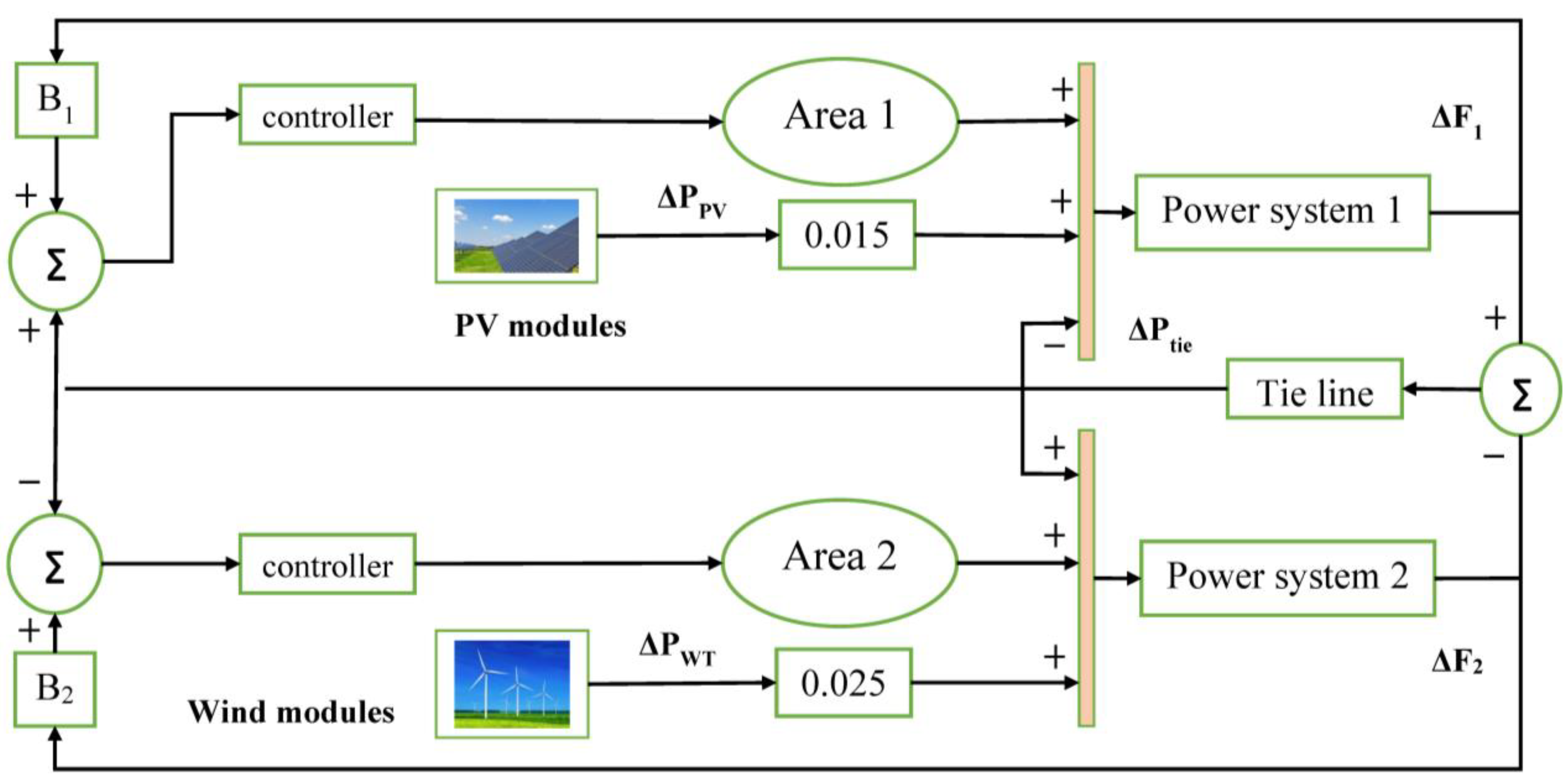
2. The Proposed Power System Modeling
2.1. Models of Dynamic Subsystems
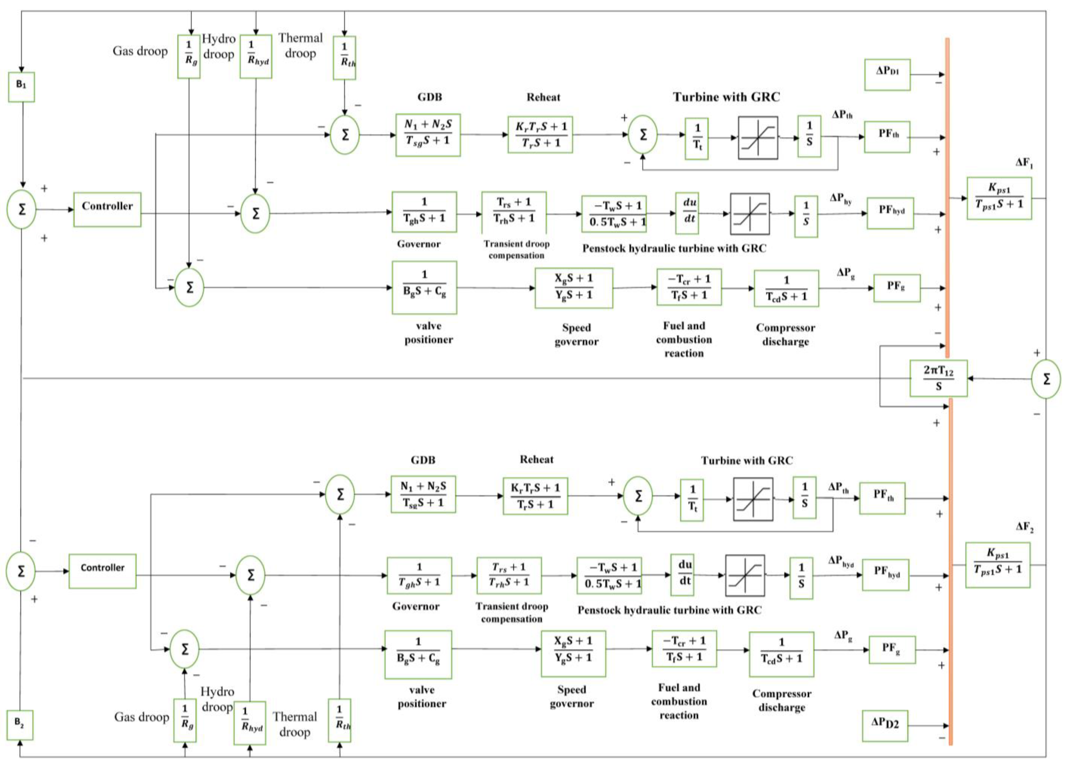
2.1.1. Thermal Power Plant Supplies 1000 MW and Includes
- Governor dead band (GDB): The GDB non-linearity formulas could be simplified as a function of changes and change rates in speeds [21]. With the aid of the Fourier series, the transfer function of a GDB with 0.5% backlash is derived as:
- Reheat is modeled using the first-order transfer function:
- Turbine with GRC
2.1.2. Hydraulic Power Plant Supplies 500 MW and Includes
- A Governor is modeled using the first-order transfer function, with a time constant for a hydro turbine governor Tgh = 0.2 s.
- Transient droop compensation is modeled using a first-order transfer function, with hydro turbine speed governor reset time Trs and a time constant of transient droop Trh of 4.9 and 28.749 s, respectively.
- Penstock hydraulic turbine with GRC
2.1.3. Gas Power Station Supplies 240 MW and Includes
- The valve positioner is modeled using the first-order transfer function with a time constant of the valve positioner Bg and the gas turbine valve positioner Cg of 0.049 and 1 s, respectively.
- The speed governor is modeled using the first-order transfer function with lead and a lag time constant of the gas turbine governor Xg, Yg of 0.6 and 1.1 s, respectively.
- Fuel and combustion reactions are modeled using the first-order transfer function with a gas turbine combustion reaction time delay Tcr and gas turbine fuel time constant Tf of 0.01 and 0.239 s, respectively.
- Compressor discharge is modeled using the first-order transfer function with compressor discharge volume time constant Tcd of 0.2 s.
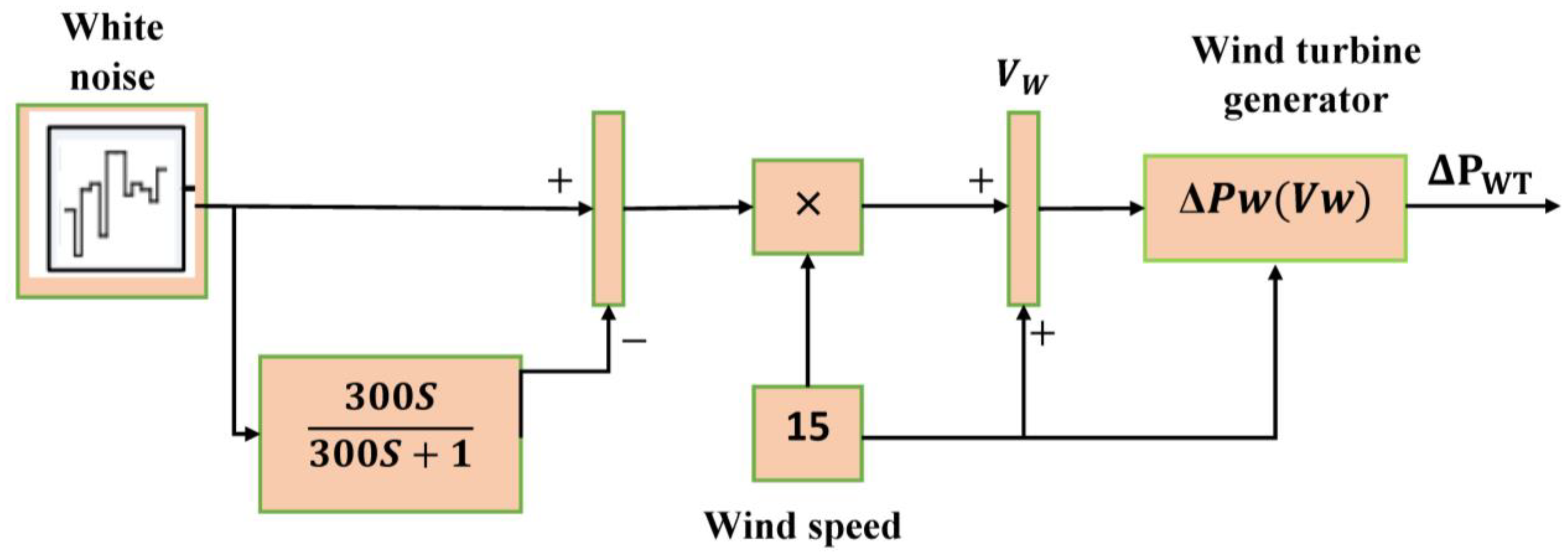
2.2. Wind Generation Model
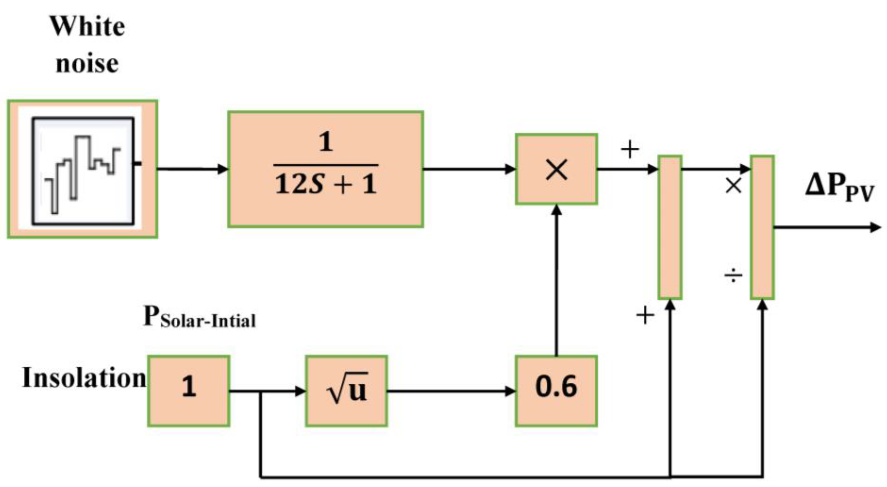
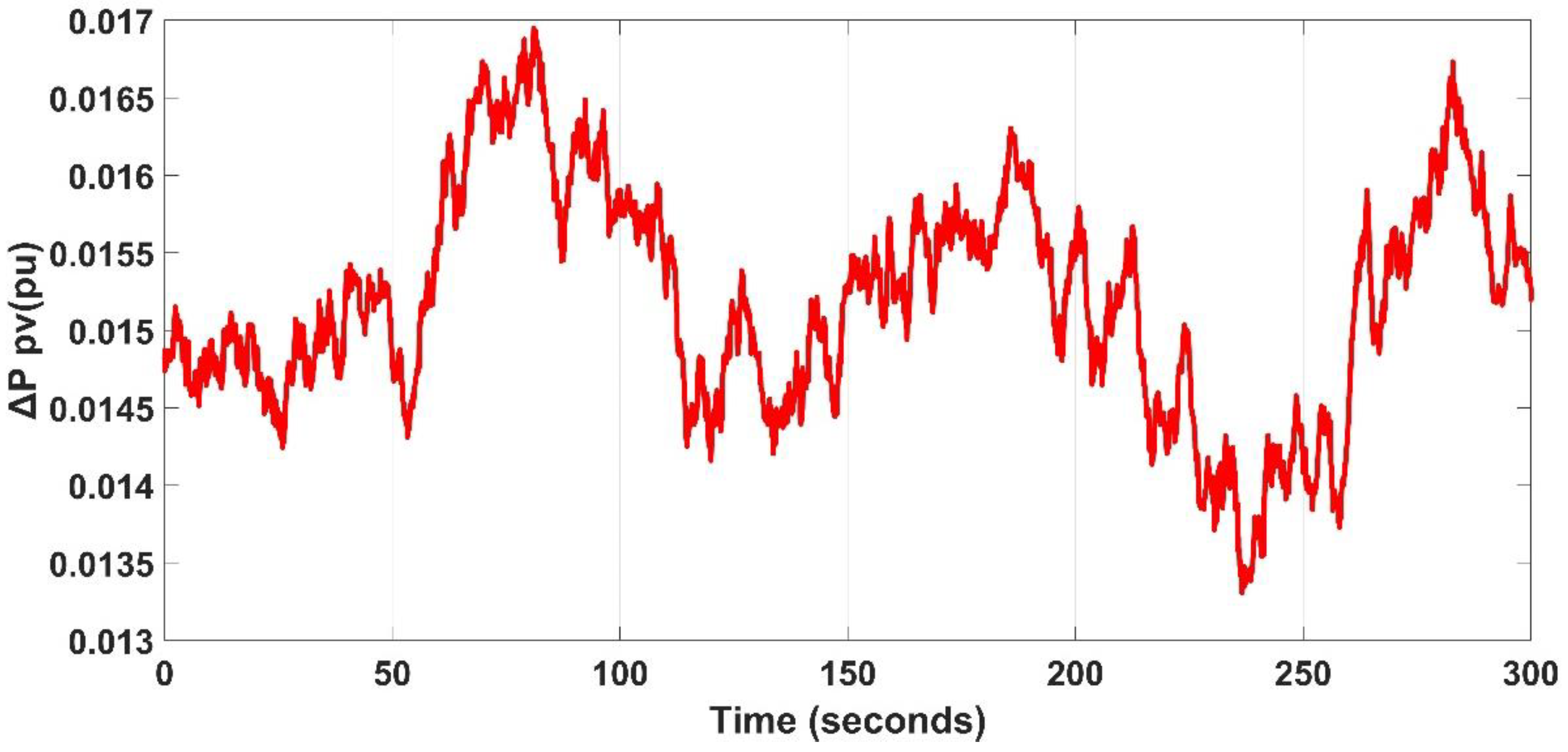
2.3. PV Generation Model
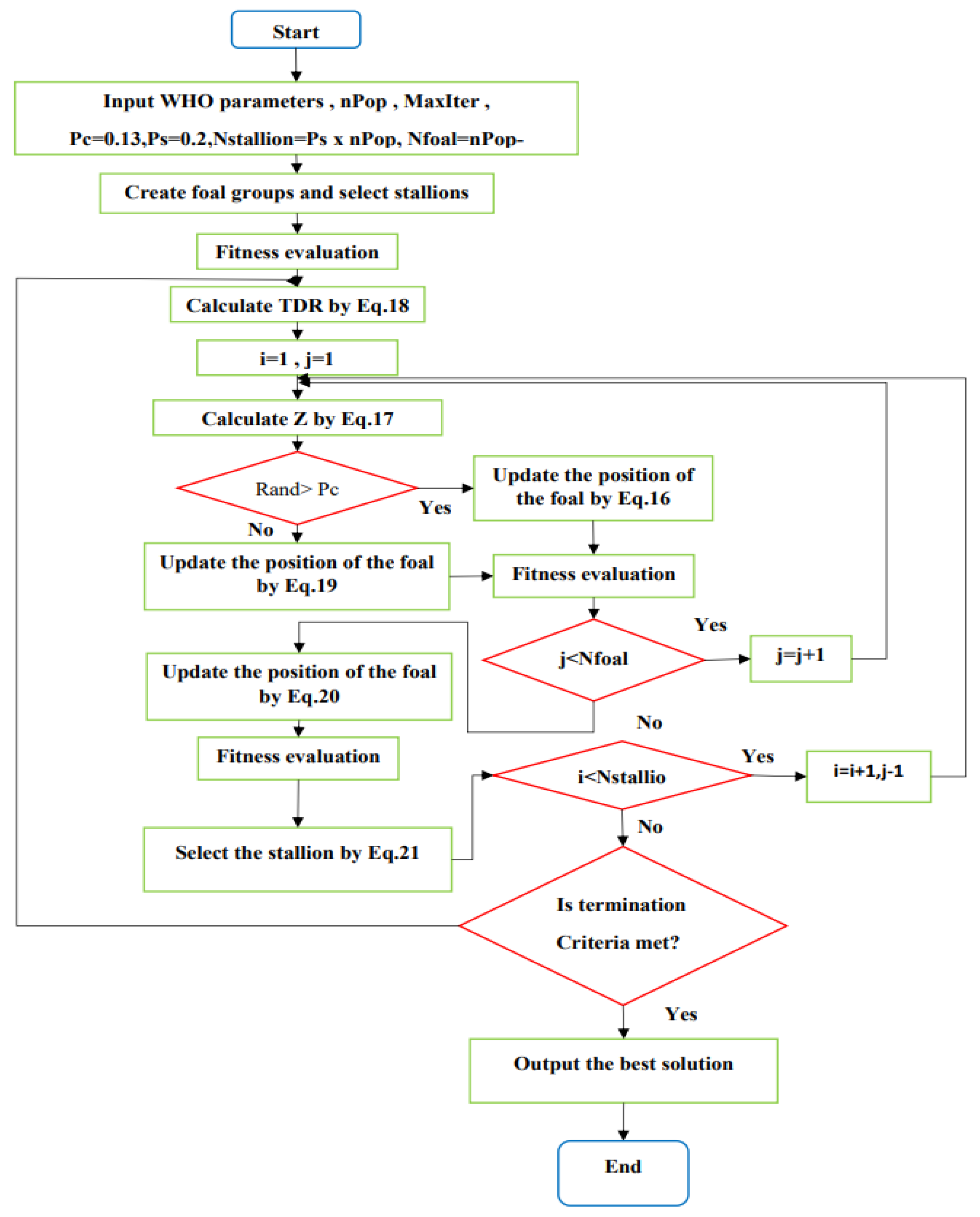
3. Wild Horse Optimization Algorithm
3.1. Population Initialization
3.2. Grazing Behavior
3.3. Behavior of Horse Mating
3.4. Group Leadership
3.5. Leaders Exchange and Selection
4. Structure of the Controller and Problem Formulation
5. Results of Simulation and Discussions
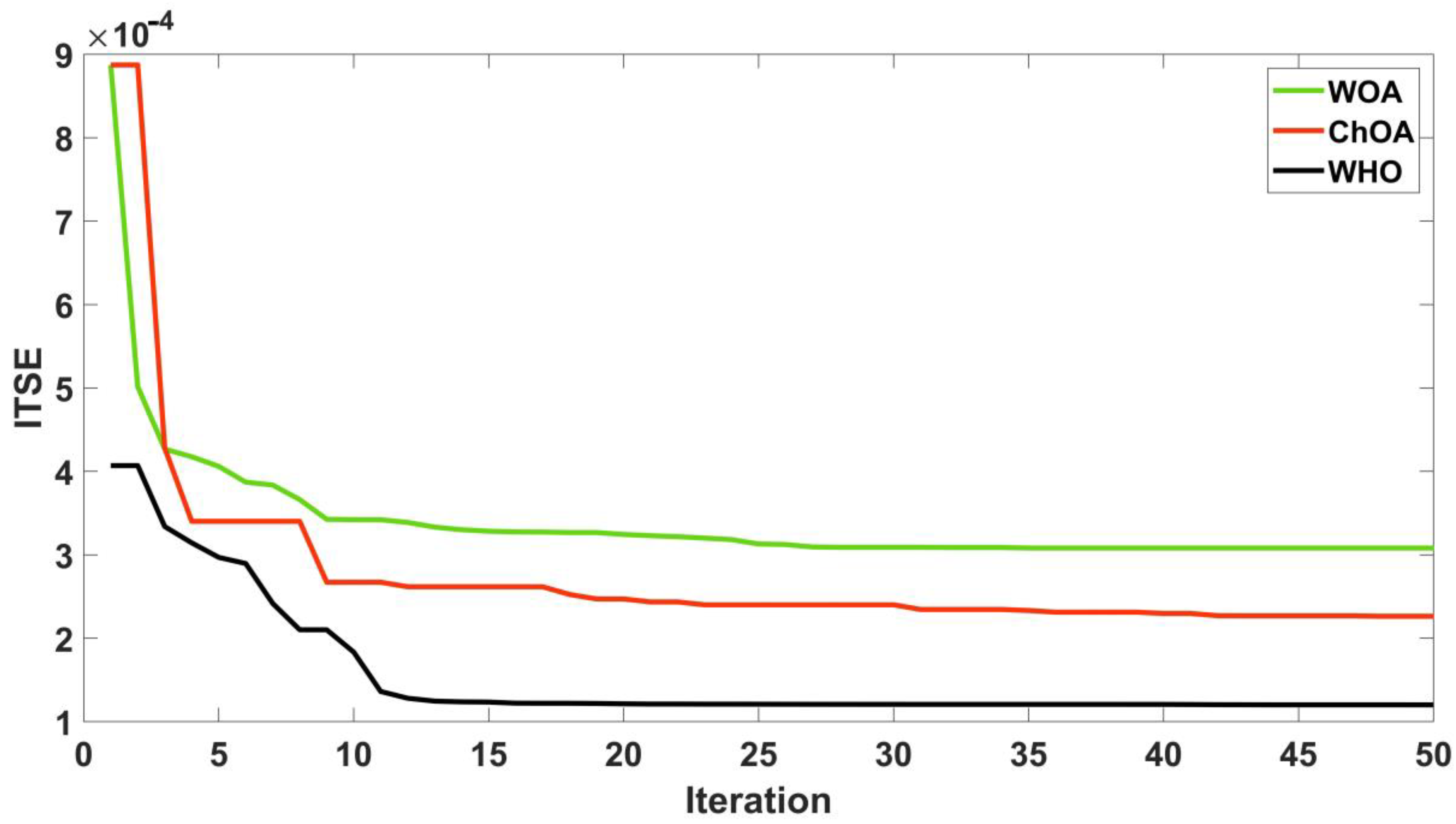
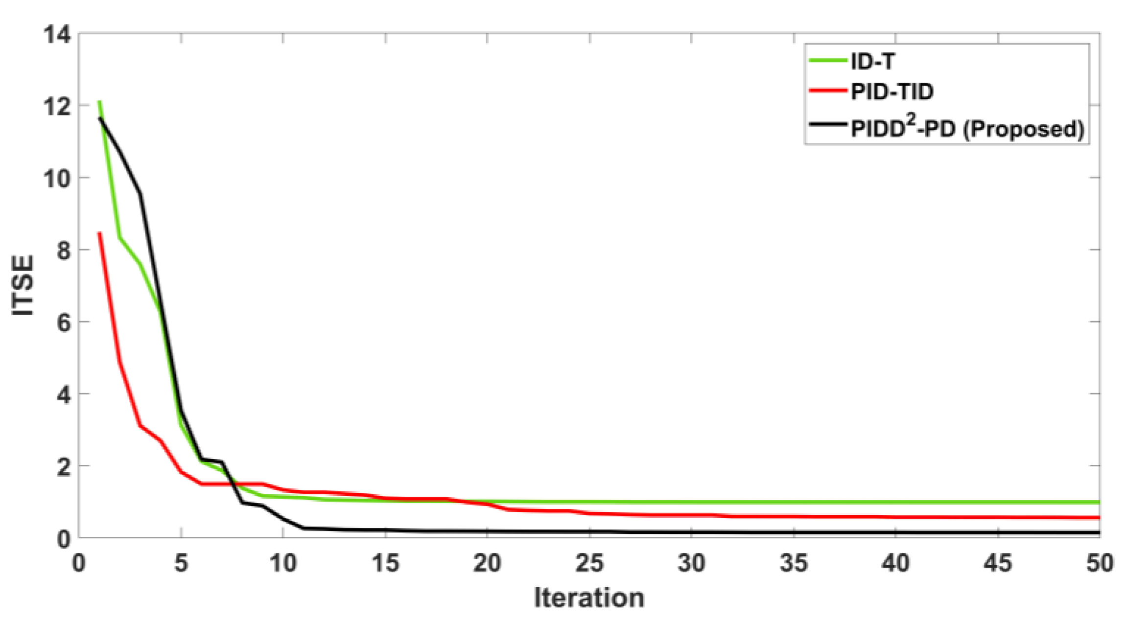
5.1. Performance Analysis of the WHO
5.2. Simulation Results and Discussions
- Scenario I: Evaluation of system dynamic response under load variation types;
- Scenario II: Evaluation of system dynamic response using RESs disturbances;
- Scenario III: Evaluation of system dynamic response with RESs disturbances, taking into consideration the communication time delay (CTD), applied to the proposed controller output;
- Scenario IV: Evaluation of system dynamic response based on RESs disturbances and changes in system settings.
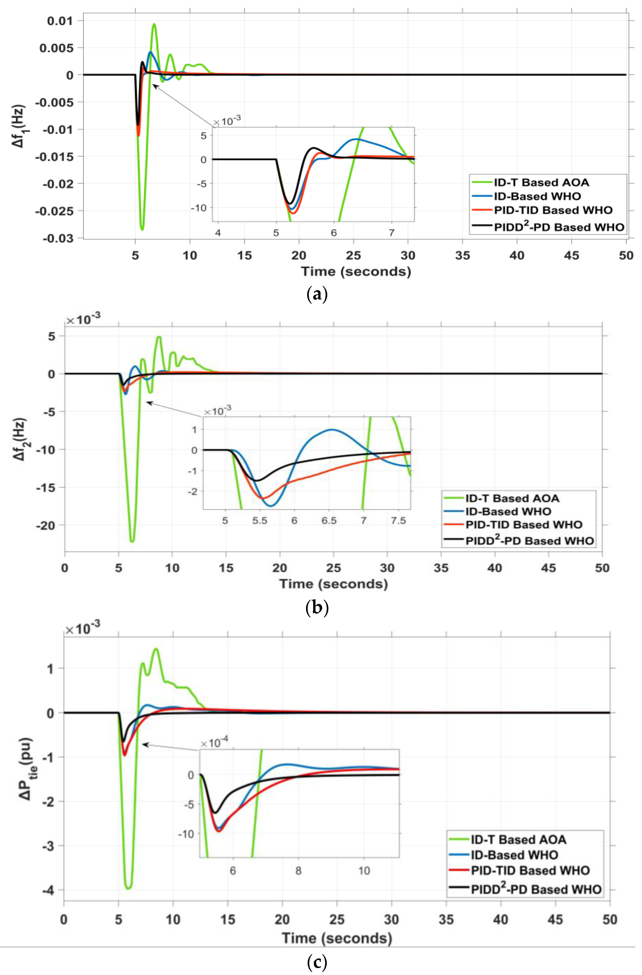
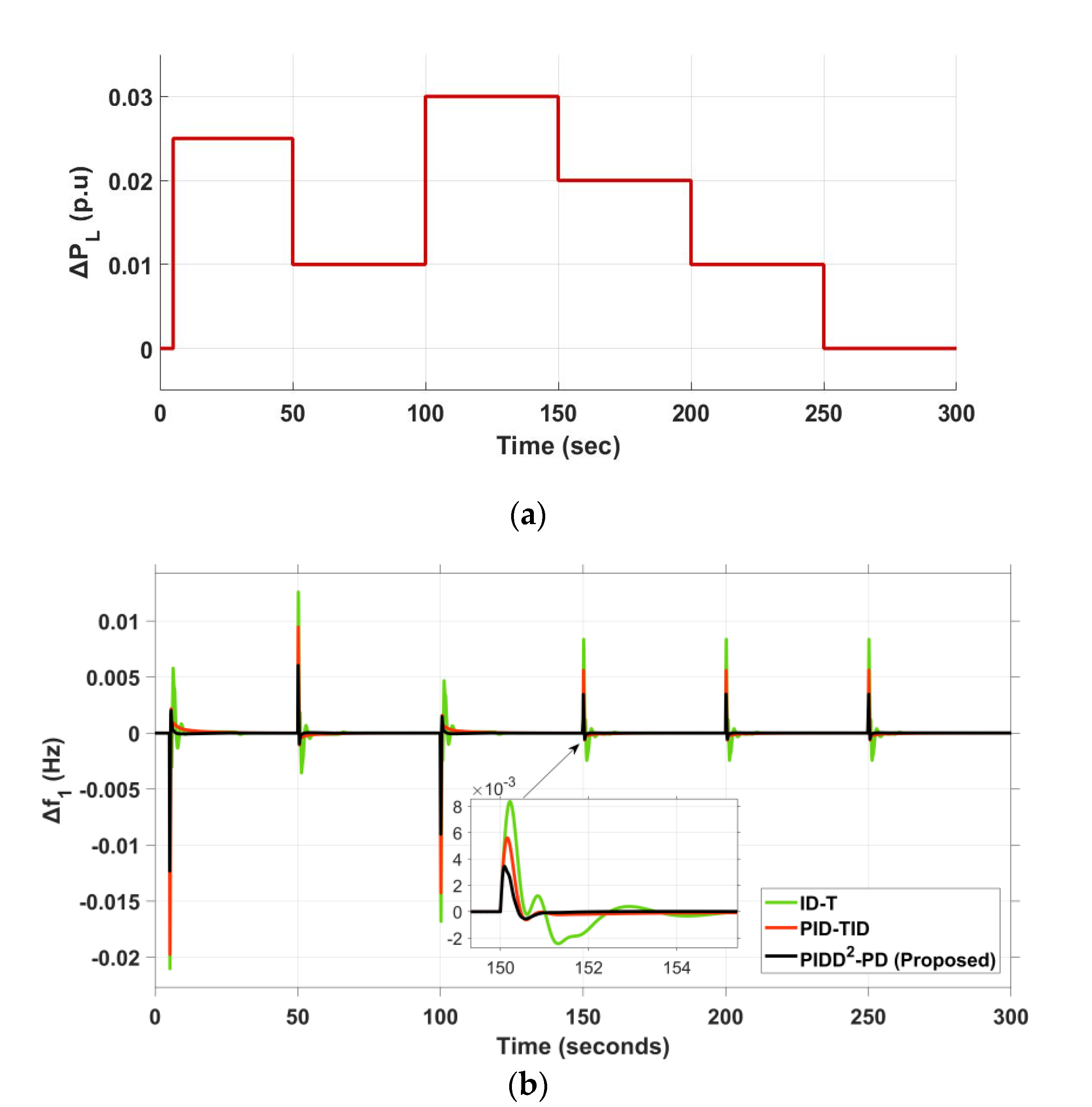
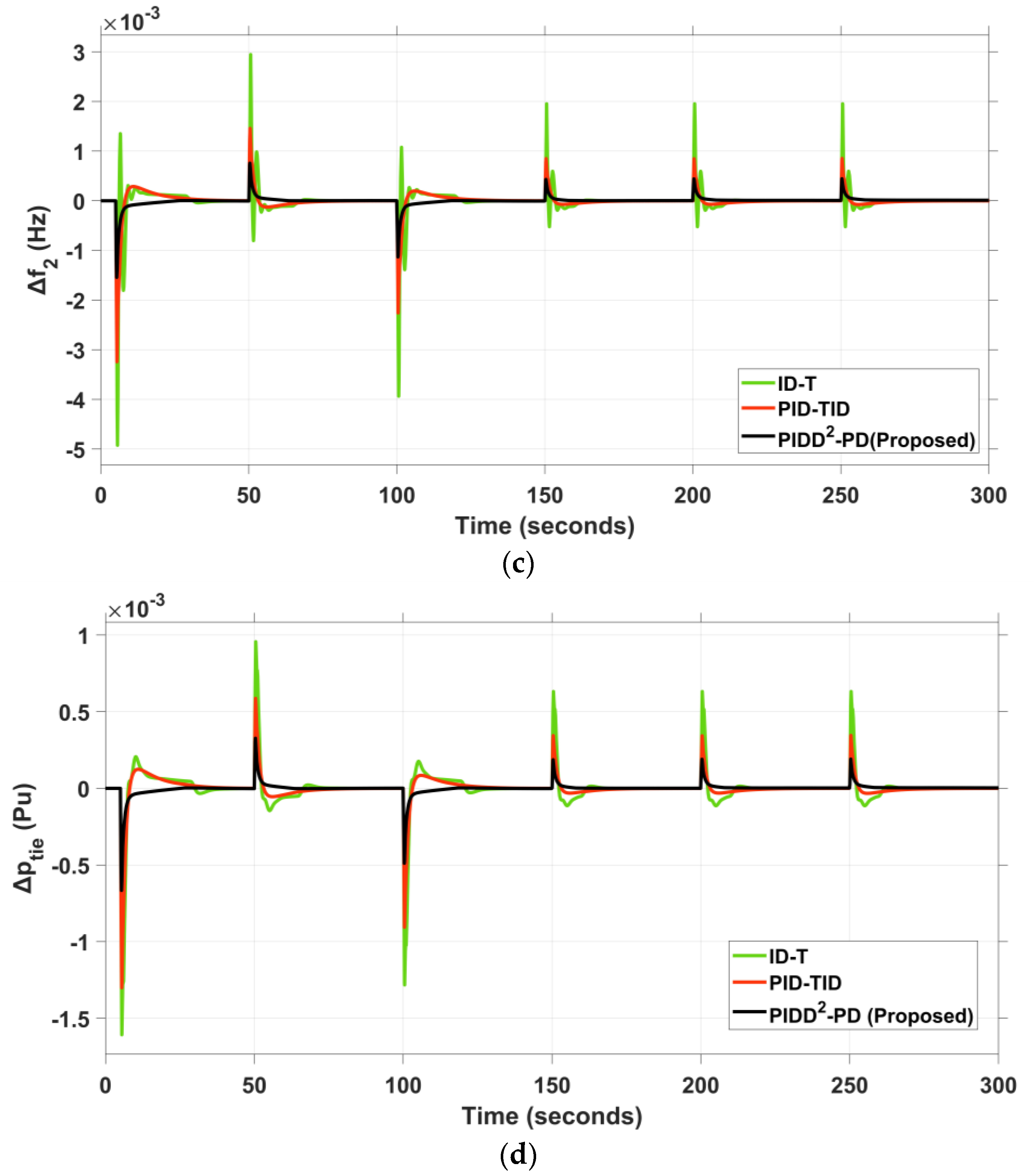
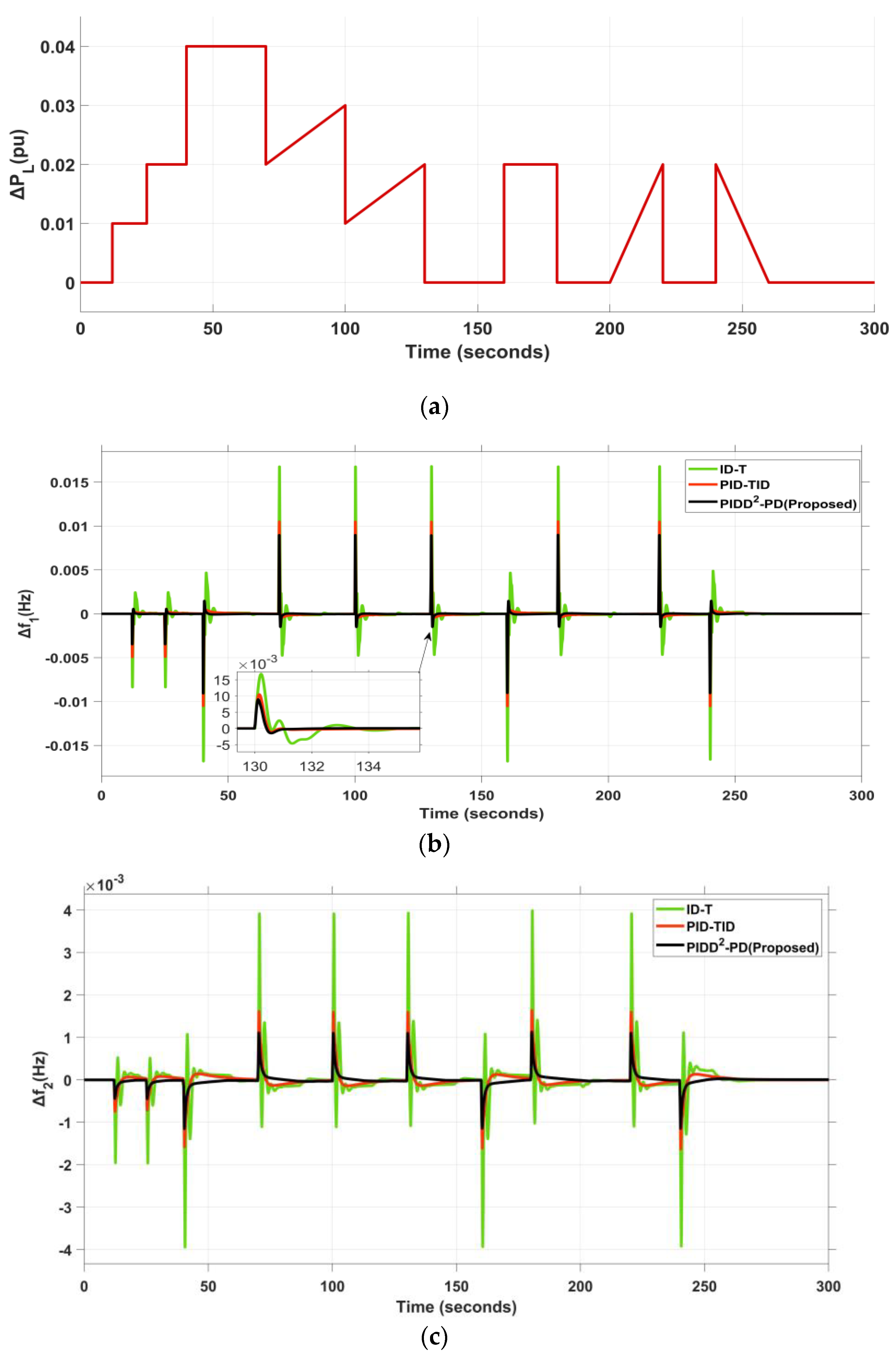
5.2.1. Scenario I: Evaluation of System Dynamic Response under Load Variation Types
5.2.2. Scenario II: Performance Evaluation Based on RESs Penetration
5.2.3. Scenario III: Evaluation of Performance Using RESs Disturbances and Communication Time Delay (CTD) on the Signal Output of the Controller
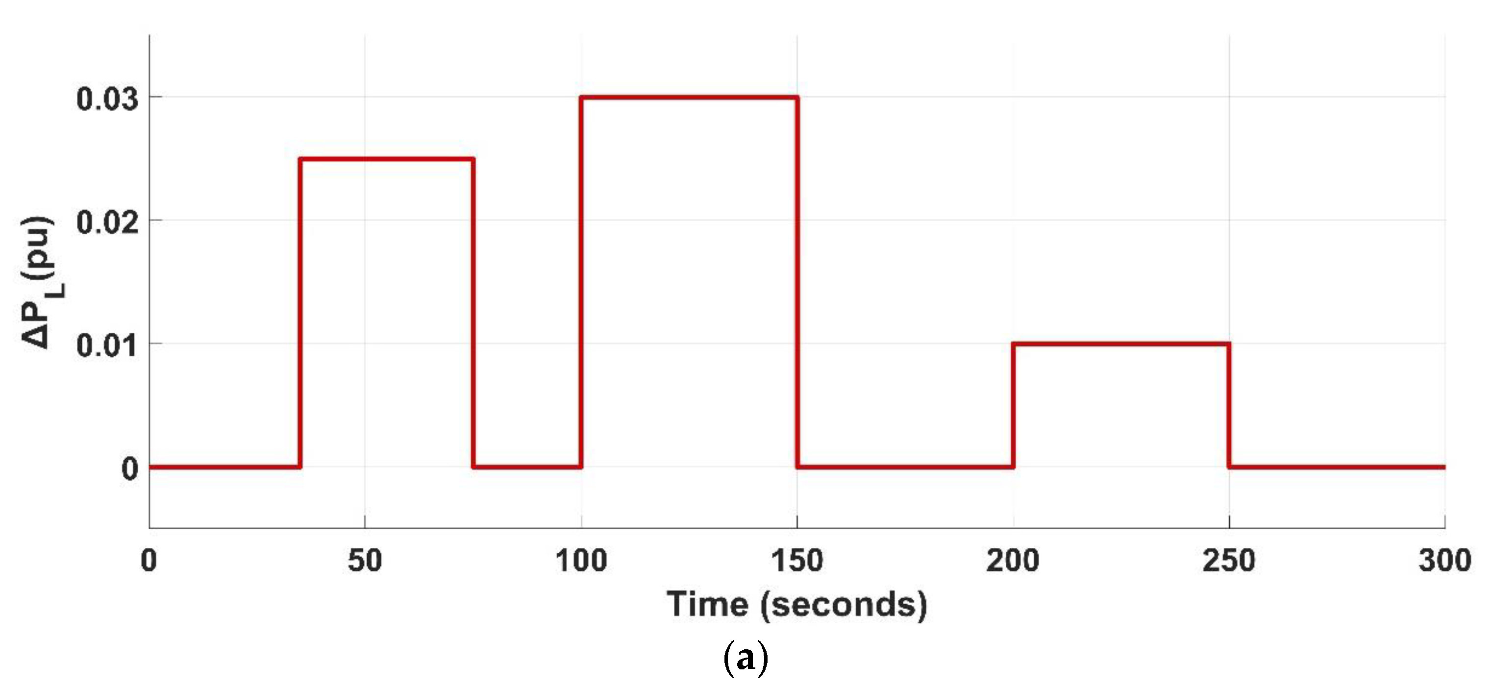
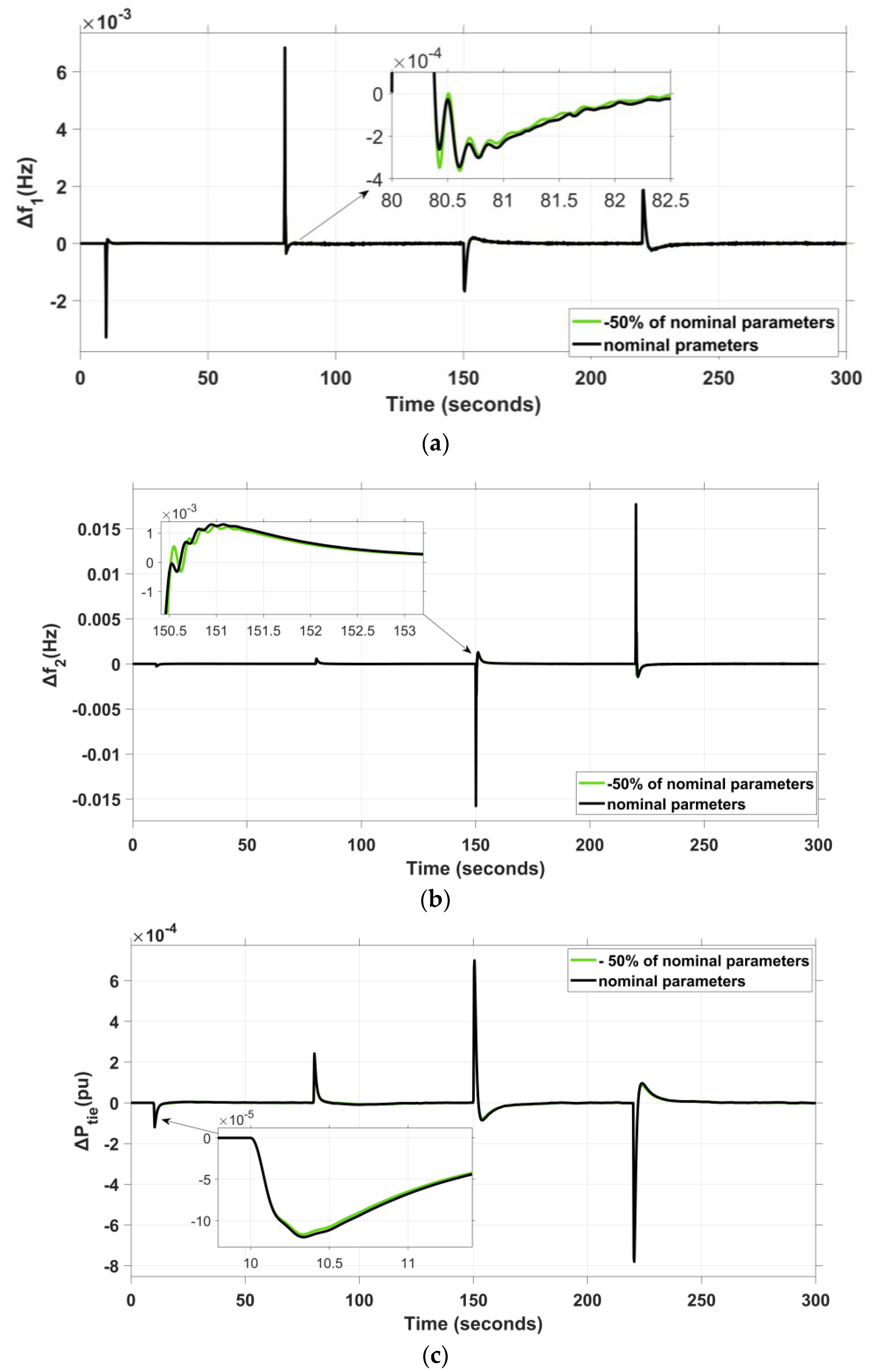
5.2.4. Scenario IV: Performance Evaluation for RESs and Changes in System Parameters
6. Conclusions
Author Contributions
Funding
Institutional Review Board Statement
Informed Consent Statement
Data Availability Statement
Conflicts of Interest
Nomenclature
| AOA | Archimedes Optimization Algorithm |
| AT | The rotor swept area (m2) |
| B1, B2 | Frequency bias coefficients |
| ChOA | Chimp Optimization Algorithm |
| CP | The power coefficient of the rotor blades |
| CTD | Communication time delay |
| FF | Fitness function |
| FO | Fractional order |
| FOC | FO calculus |
| FOPID | Fractional order proportional derivative |
| GDB | Governor dead band |
| GRC | Generation rate constraint, % (p.u) |
| H | Total number of groups |
| ID-T | Integral derivative—tilted |
| I-PD | Integral-proportional derivative |
| it | Iteration |
| I-TD | Integral-tilted derivative |
| ITSE | Integral time squared error |
| kd | Derivative gain of PD |
| KD, KDD | Derivative gains of PIDD2 |
| KI | Integral gain of PIDD2 |
| KP | Proportional gain of PIDD2 |
| kp | The proportional gain of PD |
| LFC | Load frequency control |
| maxit | Maximum number of iterations |
| Max.OS | Maximum overshoot |
| MSLD | Multi-step load disturbances |
| Max.US | Maximum undershoot |
| Nd, Ndd | Filters’ coefficients of the PIDD2 |
| nf | Filters’ coefficients of the PD |
| PD | Proportional derivative |
| PID | Proportional integral derivative |
| PIDD2 | Proportional integral derivative—second derivative |
| PV | Photovoltaics |
| Q | Population size |
| RESs | Renewable energy sources |
| RLD | Random load disturbances |
| rT | The rotor radius |
| SLD | Step load disturbances |
| SR | Number of stallions in the population |
| Set-Time | Settling time |
| TDC | Transient droop compensation |
| TID | Tilted integral derivative |
| Ts | Simulation time |
| VW | The rated wind speed (m/s) |
| WHO | Wild Horse Optimization |
| WOA | Whale Optimization Algorithm |
| Z | Randomly selected adaptive mechanism |
| β | The pitch angle |
| ΔF1 | The frequency deviation in Area 1 (Hz) |
| ΔF2 | The frequency deviation in Area 2 (Hz) |
| ΔPtie | The tie-line power deviation (p.u) |
| λ | The tip-speed ratio (TSR) |
| λI | The intermittent TSR |
| ρ | Air density (Kg/m3) |
References
- Magdy, G.; Mohamed, E.A.; Shabib, G.; Elbaset, A.A.; Mitani, Y. Microgrid dynamic security considering high penetration of renewable energy. Prot. Control. Mod. Power Syst. 2018, 3, 23. [Google Scholar] [CrossRef]
- Yang, Z.; Ghadamyari, M.; Khorramdel, H.; Alizadeh, S.M.S.; Pirouzi, S.; Milani, M.; Banihashemi, F.; Ghadimi, N. Robust multi-objective optimal design of islanded hybrid system with renewable and diesel sources/stationary and mobile energy storage systems. Renew. Sustain. Energy Rev. 2021, 148, 111295. [Google Scholar] [CrossRef]
- Dehghani, M.; Ghiasi, M.; Niknam, T.; Kavousi-Fard, A.; Shasadeghi, M.; Ghadimi, N.; Taghizadeh-Hesary, F. Blockchain-Based Securing of Data Exchange in a Power Transmission System Considering Congestion Management and Social Welfare. Sustainability 2021, 13, 90. [Google Scholar] [CrossRef]
- Magdy, G.; Shabib, G.; Elbaset, A.A.; Mitani, Y. Optimized coordinated control of LFC and SMES to enhance frequency stability of a real multi-source power system considering high renewable energy penetration. Prot. Control. Mod. Power Syst. 2018, 3, 39. [Google Scholar] [CrossRef] [Green Version]
- Khamies, M.; Magdy, G.; Kamel, S.; Khan, B. Optimal Model Predictive and Linear Quadratic Gaussian Control for Frequency Stability of Power Systems Considering Wind Energy. IEEE Access 2021, 9, 116453–116474. [Google Scholar] [CrossRef]
- Jagatheesan, K.; Anand, B.; Dey, N.; Ashour, A.S.; Balas, V.E. Load Frequency Control of Hydro-Hydro System with Fuzzy Logic Controller Considering Non-linearity. In Recent Developments and the New Direction in Soft-Computing Foundations and Applications; Springer: Cham, Switzerland, 2018; pp. 307–318. [Google Scholar]
- Nguyen, G.N.; Jagatheesan, K.; Ashour, A.S.; Anand, B.; Dey, N. Ant Colony Optimization Based Load Frequency Control of Multi-area Interconnected Thermal Power System with Governor Dead-Band Nonlinearity. In Smart Trends in Systems, Security and Sustainability; Springer: Singapore, 2018; pp. 157–167. [Google Scholar]
- Dritsas, L.; Kontouras, E.; Vlahakis, E.; Kitsios, I.; Halikias, G.; Tzes, A. Modelling issues and aggressive robust load frequency control of interconnected electric power systems. Int. J. Control 2022, 95, 753–767. [Google Scholar] [CrossRef]
- Tasnin, W.; Saikia, L.C.; Raju, M. Deregulated AGC of multi-area system incorporating dish-Stirling solar thermal and geothermal power plants using fractional order cascade controller. Int. J. Electr. Power Energy Syst. 2018, 101, 60–74. [Google Scholar] [CrossRef]
- Sharma, M.; Dhundhara, S.; Arya, Y.; Prakash, S. Frequency excursion mitigation strategy using a novel COA optimised fuzzy controller in wind integrated power systems. IET Renew. Power Gener. 2020, 14, 4071–4085. [Google Scholar] [CrossRef]
- Nandi, M.; Shiva, C.K.; Mukherjee, V. Moth-Flame Algorithm for TCSC- and SMES-Based Controller Design in Automatic Generation Control of a Two-Area Multi-unit Hydro-power System. Iran. J. Sci. Technol. 2020, 44, 1173–1196. [Google Scholar] [CrossRef]
- Jagatheesan, K.; Baskaran, A.; Dey, N.; Ashour, A.S.; Balas, V.E. Load frequency control of multi-area interconnected thermal power system: Artificial intelligence-based approach. Int. J. Autom. Control 2018, 12, 126–152. [Google Scholar] [CrossRef]
- Eltamaly, A.M.; Zaki Diab, A.A.; Abo-Khalil, A.G. Robust Control Based on H∞ and Linear Quadratic Gaussian of Load Frequency Control of Power Systems Integrated with Wind Energy System. In Control and Operation of Grid-Connected Wind Energy Systems; Springer: Cham, Switzerland, 2021; pp. 73–86. [Google Scholar]
- Habib, D. Optimal Control of PID-FUZZY based on Gravitational Search Algorithm for Load Frequency Control. Int. J. Eng. Res. 2019, 8, 50013–50022. [Google Scholar]
- Yakout, A.H.; Kotb, H.; Hasanien, H.M.; Aboras, K.M. Optimal Fuzzy PIDF Load Frequency Controller for Hybrid Microgrid System Using Marine Predator Algorithm. IEEE Access 2021, 9, 54220–54232. [Google Scholar] [CrossRef]
- Magdy, G.; Mohamed, E.A.; Shabib, G.; Elbaset, A.A.; Mitani, Y. SMES based a new PID controller for frequency stability of a real hybrid power system considering high wind power penetration. IET Renew. Power Gener. 2018, 12, 1304–1313. [Google Scholar] [CrossRef]
- Sharma, J.; Hote, Y.V.; Prasad, R. Robust PID Load Frequency Controller Design with Specific Gain and Phase Margin for Multi-area Power Systems. IFAC-Pap. 2018, 51, 627–632. [Google Scholar] [CrossRef]
- Topno, P.N.; Chanana, S. Differential evolution algorithm based tilt integral derivative control for LFC problem of an interconnected hydro-thermal power system. J. Vib. Control 2017, 24, 3952–3973. [Google Scholar] [CrossRef]
- Khokhar, B.; Dahiya, S.; Parmar, K.P.S. Load Frequency Control of a Multi-Microgrid System Incorporating Electric Vehicles. Electr. Power Compon. Syst. 2021, 49, 867–883. [Google Scholar] [CrossRef]
- Elmelegi, A.; Mohamed, E.A.; Aly, M.; Ahmed, E.M.; Mohamed, A.A.A.; Elbaksawi, O. Optimized Tilt Fractional Order Cooperative Controllers for Preserving Frequency Stability in Renewable Energy-Based Power Systems. IEEE Access 2021, 9, 8261–8277. [Google Scholar] [CrossRef]
- Morsali, J.; Zare, K.; Tarafdar Hagh, M. Comparative performance evaluation of fractional order controllers in LFC of two-area diverse-unit power system with considering GDB and GRC effects. J. Electr. Syst. Inf. Technol. 2018, 5, 708–722. [Google Scholar] [CrossRef]
- Mohamed, E.A.; Ahmed, E.M.; Elmelegi, A.; Aly, M.; Elbaksawi, O.; Mohamed, A.A.A. An Optimized Hybrid Fractional Order Controller for Frequency Regulation in Multi-Area Power Systems. IEEE Access 2020, 8, 213899–213915. [Google Scholar] [CrossRef]
- Ali, M.; Kotb, H.; Aboras, K.M.; Abbasy, N.H. Design of Cascaded PI-Fractional Order PID Controller for Improving the Frequency Response of Hybrid Microgrid System Using Gorilla Troops Optimizer. IEEE Access 2021, 9, 150715–150732. [Google Scholar] [CrossRef]
- Prakash, A.; Murali, S.; Shankar, R.; Bhushan, R. HVDC tie-link modeling for restructured AGC using a novel fractional order cascade controller. Electr. Power Syst. Res. 2019, 170, 244–258. [Google Scholar] [CrossRef]
- Saha, A.; Saikia, L.C. Load frequency control of a wind-thermal-split shaft gas turbine-based restructured power system integrating FACTS and energy storage devices. Int. Trans. Electr. Energy Syst. 2019, 29, e2756. [Google Scholar] [CrossRef]
- Mohamed, T.H.; Shabib, G.; Abdelhameed, E.H.; Khamies, M.; Qudaih, Y. Load Frequency Control in Single Area System Using Model Predictive Control and Linear Quadratic Gaussian Techniques. Int. J. Electr. Energy 2015, 3, 141–143. [Google Scholar] [CrossRef]
- Elkasem, A.H.A.; Khamies, M.; Hassan, M.H.; Agwa, A.M.; Kamel, S. Optimal Design of TD-TI Controller for LFC Considering Renewables Penetration by an Improved Chaos Game Optimizer. Fractal Fract. 2022, 6, 220. [Google Scholar] [CrossRef]
- Daraz, A.; Malik, S.A.; Mokhlis, H.; Haq, I.U.; Laghari, G.F.; Mansor, N.N. Fitness Dependent Optimizer-Based Automatic Generation Control of Multi-Source Interconnected Power System with Non-Linearities. IEEE Access 2020, 8, 100989–101003. [Google Scholar] [CrossRef]
- Singh, K.; Amir, M.; Ahmad, F.; Khan, M.A. An Integral Tilt Derivative Control Strategy for Frequency Control in Multimicrogrid System. IEEE Syst. J. 2021, 15, 1477–1488. [Google Scholar] [CrossRef]
- Kumari, S.; Shankar, G.; Das, B. Integral-Tilt-Derivative Controller Based Performance Evaluation of Load Frequency Control of Deregulated Power System. In Modeling, Simulation and Optimization; Springer: Singapore, 2021; pp. 189–200. [Google Scholar]
- Ahmed, M.; Magdy, G.; Khamies, M.; Kamel, S. Modified TID controller for load frequency control of a two-area interconnected diverse-unit power system. Int. J. Electr. Power Energy Syst. 2022, 135, 107528. [Google Scholar] [CrossRef]
- Pahadasingh, S. TLBO Based CC-PID-TID Controller for Load Frequency Control of Multi Area Power System. In Proceedings of the 2021 1st Odisha International Conference on Electrical Power Engineering, Communication and Computing Technology (ODICON), Bhubaneswar, India, 8–9 January 2021. [Google Scholar]
- Paliwal, N.; Srivastava, L.; Pandit, M. Application of grey wolf optimization algorithm for load frequency control in multi-source single area power system. Evol. Intell. 2020, 15, 563–584. [Google Scholar] [CrossRef]
- Revathi, D.; Mohan Kumar, G. Analysis of LFC in PV-thermal-thermal interconnected power system using fuzzy gain scheduling. Int. Trans. Electr. Energy Syst. 2020, 30, e12336. [Google Scholar] [CrossRef]
- Jagatheesan, K.; Anand, B.; Dey, N.; Gaber, T.; Hassanien, A.E.; Kim, T.H. A Design of PI Controller using Stochastic Particle Swarm Optimization in Load Frequency Control of Thermal Power Systems. In Proceedings of the 2015 Fourth International Conference on Information Science and Industrial Applications (ISI), Busan, Korea, 20–22 September 2015. [Google Scholar]
- Ah, G.H.; Li, Y.Y. Ant lion optimized hybrid intelligent PID-based sliding mode controller for frequency regulation of interconnected multi-area power systems. Trans. Inst. Meas. Control 2020, 42, 1594–1617. [Google Scholar] [CrossRef]
- Patel, N.C.; Sahu, B.K.; Khamari, R.C. TLBO Designed 2-DOFPIDF Controller for LFC of Multi-area Multi-source Power System. In Innovation in Electrical Power Engineering, Communication, and Computing Technology; Springer: Singapore, 2022; pp. 269–282. [Google Scholar]
- Aryan, P.; Ranjan, M.; Shankar, R. Deregulated LFC scheme using equilibrium optimized Type-2 fuzzy controller. In Proceedings of the International conference on Innovative Development and Engineering Applications, Gaya, India, 8–10 February 2021. [Google Scholar]
- Khokhar, B.; Dahiya, S.S.; Singh Parmar, K.P. Atom search optimization based study of frequency deviation response of a hybrid power system. In Proceedings of the 2020 IEEE 9th Power India International Conference (PIICON), Murthal, India, 28 February–1 March 2020; pp. 1–5. [Google Scholar]
- Naruei, I.; Keynia, F. Wild horse optimizer: A new meta-heuristic algorithm for solving engineering optimization problems. Eng. Comput. 2021, 1–32. [Google Scholar] [CrossRef]
- Khishe, M.; Mosavi, M.R. Chimp optimization algorithm. Expert Syst. Appl. 2020, 149, 113338. [Google Scholar] [CrossRef]
- Mirjalili, S.; Lewis, A. The Whale Optimization Algorithm. Adv. Eng. Softw. 2016, 95, 51–67. [Google Scholar] [CrossRef]
- Parmar, K.P.S.; Majhi, S.; Kothari, D.P. LFC of an Interconnected Power System with Thyristor Controlled Phase Shifter in the Tie Line. Int. J. Comput. Appl. 2012, 41, 27–30. [Google Scholar]
- Magdy, G.; Shabib, G.; Elbaset, A.A.; Kerdphol, T.; Qudaih, Y.; Mitani, Y. Decentralized optimal LFC for a real hybrid power system considering renewable energy sources. J. Eng. Sci. Technol. 2019, 14, 682–697. [Google Scholar]
- Ali, M.; Kotb, H.; AboRas, M.K.; Abbasy, H.N. Frequency regulation of hybrid multi-area power system using wild horse optimizer based new combined Fuzzy Fractional-Order PI and TID controllers. Alex. Eng. J. 2022, 61, 12187–12210. [Google Scholar] [CrossRef]
- Kalyan, C.N.S.; Suresh, C.V. PIDD controller for AGC of nonlinear system with PEV integration and AC-DC links. In Proceedings of the 2021 International Conference on Sustainable Energy and Future Electric Transportation (SEFET), Hyderabad, India, 21–23 January 2021. [Google Scholar]


| Model | Transfer Function | Parameter | Value | Description |
|---|---|---|---|---|
| Power system 1 | 11.49 s 68.9655 | Power system time constants Power system gains | ||
| Power system 2 | ||||
| T-line | 0.0433 | Synchronization factor | ||
| 0.4312 | Coefficient values of frequency bias |
| Parameter | Value | Parameter | Value |
|---|---|---|---|
| 750 kW | 116 | ||
| 15 m/s | 0.4 | ||
| 22.9 m | 0 | ||
| 1.225 kg/m3 | 5 | ||
| 1684 m2 | 21 | ||
| 22.5 r.p.m | 0.1405 | ||
| −0.6175 | |||
| WHO Parameter | Value |
|---|---|
| SR | 0.2 |
| H | 6 |
| Q | 30 |
| Number of foals | 24 |
| R | 0.2372 |
| WP | [2, 1.83, 0, 2, 2, 2, 0, 0, 0, 1, 0, 0, 0, 4.7, 20, 20, 3.19, 20, 20, 12.7] |
| AREA 1 | |||||||||
|---|---|---|---|---|---|---|---|---|---|
| Algorithm | PD1 | PIDD21 | |||||||
| kp1 | kd1 | nf1 | KP1 | KI1 | KD1 | KDD1 | Nd1 | Ndd1 | |
| WOA | 14.253 | 4.4785 | 500 | 50 | 50 | 1.7171 | 0.1 | 500 | 500 |
| ChOA | 14.564 | 0 | 500 | 50 | 0 | 6.3209 | 0.1228 | 401.6571 | 309.896 |
| WHO | 38.475 | 0.0144 | 431.882 | 41.1532 | 0.3835 | 5.6677 | 0.1 | 100 | 478.5245 |
| AREA 2 | |||||||||
| Algorithm | PD2 | PIDD22 | |||||||
| kp2 | kd2 | nf2 | KP2 | KI2 | KD2 | KDD2 | Nd2 | Ndd2 | |
| WOA | 50 | 50 | 500 | 50 | 12.451 | 4.1011 | 0.8 | 500 | 500 |
| ChOA | 0.008 | 0 | 496.631 | 0.0975 | 0.1436 | 0 | 0.2725 | 323.829 | 304.0149 |
| WHO | 0 | 17.32 | 334.76 | 50 | 7.8044 | 0.5505 | 0.1501 | 251.83 | 498.7457 |
| Optimization Techniques | ΔF1 (Hz) | ΔF2 (Hz) | ΔPtie (p.u) | ITSE | ||||||
|---|---|---|---|---|---|---|---|---|---|---|
| Max. OS | Max. US | Set-Time | Max. OS | Max. US | Set-Time | Max. OS | Max. US | Set- Time | ||
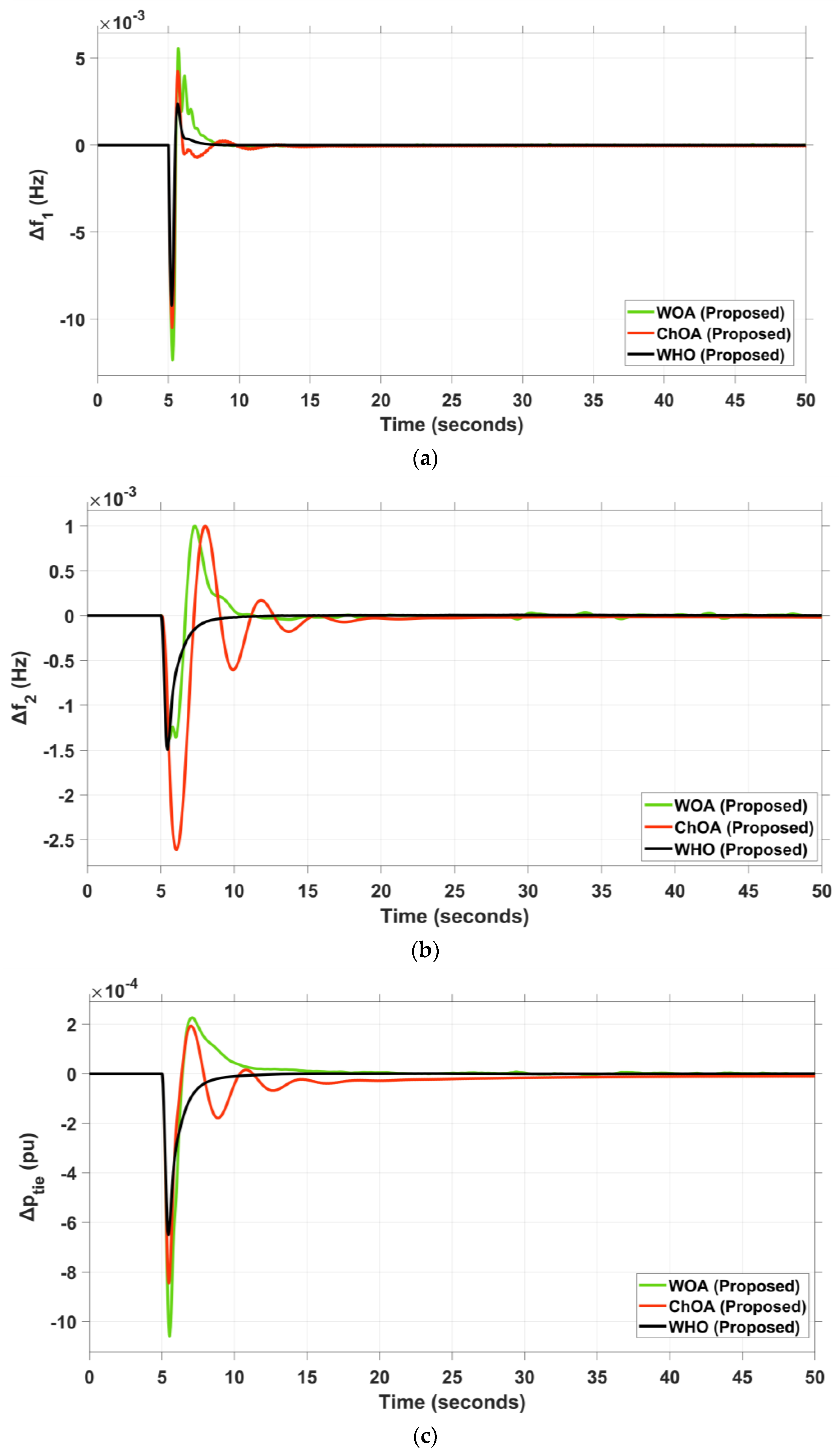
| WOA | 0.0055 | 0.0124 | 3.6 | 0.001 | 0.00137 | 15.1 | 0.00023 | 0.00106 | 12.8 | 0.0003082 |
| ChOA | 0.0042 | 0.0105 | 10.7 | 0.001 | 0.00261 | 20.8 | 0.00019 | 0.00085 | 28 | 0.0002264 |
| WHO (proposed) | 0.0024 | 0.0092 | 3.3 | 0 | 0.00149 | 7.2 | 0 | 0.00065 | 8.8 | 0.0001202 |
| AREA 1 | |||||||||
|---|---|---|---|---|---|---|---|---|---|
| Algorithm | PD1 | PIDD21 | |||||||
| kp1 | kd1 | nf1 | KP1 | KI1 | KD1 | KDD1 | Nd1 | Ndd1 | |
| PIDD2-PD (WHO) (suggested) | 38.475 | 0.0144 | 431.882 | 41.1532 | 0.3835 | 5.6677 | 0.1 | 100 | 478.5245 |
| AREA 2 | |||||||||
| Algorithm | PD2 | PIDD22 | |||||||
| kp2 | kd2 | nf2 | KP2 | KI2 | KD2 | KDD2 | Nd2 | Ndd2 | |
| PIDD2-PD (WHO) (suggested) | 0 | 17.32 | 334.76 | 50 | 7.8044 | 0.5505 | 0.1501 | 251.83 | 498.7457 |
| AREA 1 | |||||||||
| Algorithm | PID | TID | |||||||
| kp1 | ki1 | kd1 | nf1 | KT1 | n1 | KI1 | KD1 | ||
| PID-TID (WHO) | 6.1095 | 0 | 34.0678 | 489.8079 | 49.9998 | 2.5167 | 50 | 2.5459 | |
| AREA 2 | |||||||||
| Algorithm | PID | TID | |||||||
| kp2 | ki2 | kd2 | nf2 | KT2 | n2 | KI2 | KD2 | ||
| PID-TID (WHO) | 25.6245 | 12.8848 | 3.2186 | 499.8395 | 49.2407 | 2.4475 | 14.9894 | 3.8772 | |
| AREA 1 | |||||||||
| Algorithm | T | ID | |||||||
| KT1 | n1 | KI1 | KD1 | NC1 | |||||
| ID-T (WHO) | −31.4909 | 1.7755 | 39.3266 | 25.3455 | 499.3504 | ||||
| AREA 2 | |||||||||
| Algorithm | T | ID | |||||||
| KT2 | n2 | KI2 | KD2 | NC2 | |||||
| ID-T (WHO) | −15.2490 | 2.8479 | 38.8390 | 12.0328 | 336.9504 | ||||
| AREA 1 | |||||||||
| Algorithm | T | ID | |||||||
| KT1 | n1 | KI1 | KD1 | NC1 | |||||
| ID-T (AOA) | −4.9 | 2.17 | −3.4 | −3.6 | 496.9 | ||||
| AREA 2 | |||||||||
| Algorithm | T | ID | |||||||
| KT2 | n2 | KI2 | KD2 | NC2 | |||||
| ID-T (AOA) | −0.002 | 6.07 | −0.010 | −2.390 | 469.2 | ||||
| Controller | ΔF1 (Hz) | ΔF2 (Hz) | ΔPtie (p.u) | ITSE | ||||||
|---|---|---|---|---|---|---|---|---|---|---|
| Max. OS | Max. US | Set-Time | Max. OS | Max. US | Set-Time | Max. OS | Max. US | Set- Time | ||
| PIDD2-PD (WHO) (suggested) | 0.0024 | 0.0092 | 3.3 | 0 | 0.00149 | 7.2 | 0 | 0.00065 | 8.7 | 0.0001202 |
| PID-TID (WHO) | 0.0013 | 0.0112 | 16.1 | 0.00021 | 0.00235 | 18.6 | 0.00009 | 0.00096 | 20.4 | 0.0002403 |
| ID-T (AOA) | 0.009 | 0.028 | 11 | 0.005 | 0.024 | 12 | 0.001 | 0.004 | 11 | 0.001 |
| ID-T (WHO) | 0.0042 | 0.0103 | 11.8 | 0.00098 | 0.00272 | 13.3 | 0.00017 | 0.00091 | 16 | 0.0002689 |
| Controller | ΔF1 (Hz) | ΔF2 (Hz) | ΔPtie (p.u) | ITSE | |||
|---|---|---|---|---|---|---|---|
| Max. OS | Max. US | Max. OS | Max. US | Max. OS | Max. US | ||
| PIDD2-PD (WHO) (suggested) | 0.0060 | 0.0123 | 0.00076 | 0.00154 | 0.00033 | 0.00067 | 0.003442 |
| PID-TID (WHO) | 0.0095 | 0.0197 | 0.00146 | 0.00324 | 0.00059 | 0.00130 | 0.01051 |
| ID-T (WHO) | 0.0126 | 0.0210 | 0.0029 | 0.0049 | 0.00096 | 0.00161 | 0.02664 |
| Controller | ΔF1 (Hz) | ΔF2 (Hz) | ΔPtie (p.u) | ITSE | |||
|---|---|---|---|---|---|---|---|
| Max. OS | Max. US | Max. OS | Max. US | Max. OS | Max. US | ||
| PIDD2-PD (WHO) (suggested) | 0.0090 | 0.0091 | 0.00113 | 0.00115 | 0.00049 | 0.00050 | 0.01756 |
| PID-TID (WHO) | 0.0105 | 0.0105 | 0.00164 | 0.00163 | 0.00066 | 0.00065 | 0.02848 |
| ID-T (WHO) | 0.0168 | 0.0168 | 0.0040 | 0.0039 | 0.00131 | 0.00129 | 0.1063 |
| AREA 1 | |||||||||
|---|---|---|---|---|---|---|---|---|---|
| Algorithm | PD1 | PIDD21 | |||||||
| kp1 | kd1 | nf1 | KP1 | KI1 | KD1 | KDD1 | Nd1 | Ndd1 | |
| PIDD2-PD (WHO) (suggested) | 48.2812 | 6.328 | 343.1941 | 40.63 | 2.5682 | 2.1527 | 0.0084 | 140.5213 | 421.9369 |
| AREA 2 | |||||||||
| Algorithm | PD2 | PIDD22 | |||||||
| kp2 | kd2 | nf2 | KP2 | KI2 | KD2 | KDD2 | Nd2 | Ndd2 | |
| PIDD2-PD (WHO) (suggested) | 49.9496 | 2.0937 | 301.5396 | 44.5887 | 9.9736 | 9.8294 | 0 | 420.2037 | 118.7231 |
| AREA 1 | |||||||||
| Algorithm | PID | TID | |||||||
| kp1 | ki1 | kd1 | nf1 | KT1 | n1 | KI1 | KD1 | ||
| PID-TID (WHO) | 23.4461 | 0 | 26.4650 | 300 | 45.3144 | 2.5099 | 14.3536 | 0.9136 | |
| AREA 2 | |||||||||
| Algorithm | PID | TID | |||||||
| kp2 | ki2 | kd2 | nf2 | KT2 | n2 | KI2 | KD2 | ||
| PID-TID (WHO) | 33.2919 | 0.0947 | 3.9765 | 483.1653 | 40.6655 | 6.9517 | 0 | 2.4108 | |
| AREA 1 | |||||||||
| Algorithm | T | ID | |||||||
| KT1 | n1 | KI1 | KD1 | NC1 | |||||
| ID-T (WHO) | 39.9993 | 1.8675 | 39.9995 | 40 | 500 | ||||
| AREA 2 | |||||||||
| Algorithm | T | ID | |||||||
| KT2 | n2 | KI2 | KD2 | NC2 | |||||
| ID-T (WHO) | 25.3571 | 9.9994 | 39.9404 | 28.3108 | 495.5133 | ||||
| Controller | ΔF1 (Hz) | ΔF2 (Hz) | ΔPtie (p.u) | ITSE | |||
|---|---|---|---|---|---|---|---|
| Max. OS | Max. US | Max. OS | Max. US | Max. OS | Max. US | ||
| PIDD2-PD (WHO) (suggested) | 0.0157 | 0.0157 | 0.0178 | 0.0024 | 0.00064 | 0.0015 | 0.01959 |
| PID-TID (WHO) | 0.0191 | 0.0192 | 0.0218 | 0.0105 | 0.00090 | 0.00217 | 0.04153 |
| ID-T (WHO) | 0.0205 | 0.0200 | 0.0249 | 0.0077 | 0.00152 | 0.00349 | 0.08325 |
| AREA 1 | |||||||||
|---|---|---|---|---|---|---|---|---|---|
| Algorithm | PD1 | PIDD21 | |||||||
| kp1 | kd1 | nf1 | KP1 | KI1 | KD1 | KDD1 | Nd1 | Ndd1 | |
| PIDD2-PD (WHO) (suggested) | 2.7227 | 0.3027 | 195.6591 | 19.6364 | 6.3706 | 7.6158 | 0.0541 | 190.8568 | 130.8450 |
| AREA 2 | |||||||||
| Algorithm | PD2 | PIDD22 | |||||||
| kp2 | kd2 | nf2 | KP2 | KI2 | KD2 | KDD2 | Nd2 | Ndd2 | |
| PIDD2-PD (WHO) (suggested) | 7.4519 | 1.5539 | 148.7560 | 6.4190 | 12.1799 | 1.8329 | 0.0269 | 141.0946 | 100.4050 |
| AREA 1 | |||||||||
| Algorithm | PID | TID | |||||||
| kp1 | ki1 | kd1 | nf1 | KT1 | n1 | KI1 | KD1 | ||
| PID-TID (WHO) | 1.9950 | 0.0027 | 4.3505 | 375.0716 | 16.9318 | 1.738 | 3.4679 | 1.4928 | |
| AREA 2 | |||||||||
| Algorithm | PID | TID | |||||||
| kp2 | ki2 | kd2 | nf2 | KT2 | n2 | KI2 | KD2 | ||
| PID-TID (WHO) | 7.3223 | 0.0140 | 3.2081 | 312.8155 | 7.5334 | 5.1325 | 3.9343 | 1.1741 | |
| AREA 1 | |||||||||
| Algorithm | T | ID | |||||||
| KT1 | n1 | KI1 | KD1 | NC1 | |||||
| ID-T (WHO) | 5.4107 | 9.5456 | 5.0845 | 6.6880 | 389.4373 | ||||
| AREA 2 | |||||||||
| Algorithm | T | ID | |||||||
| KT2 | n2 | KI2 | KD2 | NC2 | |||||
| ID-T (WHO) | 17.4930 | 1.4958 | 4.5823 | 13.7478 | 480.3091 | ||||
| Controller | ΔF1 (Hz) | ΔF2 (Hz) | ΔPtie (p.u) | ITSE | |||
|---|---|---|---|---|---|---|---|
| Max. OS | Max. US | Max. OS | Max. US | Max. OS | Max. US | ||
| PIDD2-PD (WHO) (suggested) | 0.0148 | 0.0116 | 0.030 | 0.048 | 0.00308 | 0.00176 | 0.1488 |
| PID-TID (WHO) | 0.0222 | 0.0246 | 0.044 | 0.078 | 0.0075 | 0.0035 | 0.5603 |
| ID-T (WHO) | 0.0323 | 0.0307 | 0.052 | 0.080 | 0.0088 | 0.0055 | 0.9892 |
| Controller | ΔF1 (Hz) | ΔF2 (Hz) | ΔPtie (p.u) | ITSE | |||
|---|---|---|---|---|---|---|---|
| Max. OS | Max. US | Max. OS | Max. US | Max. OS | Max. US | ||
| PIDD2-PD (suggested) | 0.0068 | 0.0033 | 0.0177 | 0.0158 | 0.00070 | 0.00078 | 0.0167 |
| PIDD2-PD (suggested) with +50% | 0.0068 | 0.0033 | 0.0178 | 0.0159 | 0.00072 | 0.00081 | 0.0172 |
| PIDD2-PD (suggested) with −50% | 0.0068 | 0.0033 | 0.0176 | 0.0157 | 0.00065 | 0.00074 | 0.01583 |
Publisher’s Note: MDPI stays neutral with regard to jurisdictional claims in published maps and institutional affiliations. |
© 2022 by the authors. Licensee MDPI, Basel, Switzerland. This article is an open access article distributed under the terms and conditions of the Creative Commons Attribution (CC BY) license (https://creativecommons.org/licenses/by/4.0/).
Share and Cite
Khudhair, M.; Ragab, M.; AboRas, K.M.; Abbasy, N.H. Robust Control of Frequency Variations for a Multi-Area Power System in Smart Grid Using a Newly Wild Horse Optimized Combination of PIDD2 and PD Controllers. Sustainability 2022, 14, 8223. https://doi.org/10.3390/su14138223
Khudhair M, Ragab M, AboRas KM, Abbasy NH. Robust Control of Frequency Variations for a Multi-Area Power System in Smart Grid Using a Newly Wild Horse Optimized Combination of PIDD2 and PD Controllers. Sustainability. 2022; 14(13):8223. https://doi.org/10.3390/su14138223
Chicago/Turabian StyleKhudhair, Mohammed, Muhammad Ragab, Kareem M. AboRas, and Nabil H. Abbasy. 2022. "Robust Control of Frequency Variations for a Multi-Area Power System in Smart Grid Using a Newly Wild Horse Optimized Combination of PIDD2 and PD Controllers" Sustainability 14, no. 13: 8223. https://doi.org/10.3390/su14138223
APA StyleKhudhair, M., Ragab, M., AboRas, K. M., & Abbasy, N. H. (2022). Robust Control of Frequency Variations for a Multi-Area Power System in Smart Grid Using a Newly Wild Horse Optimized Combination of PIDD2 and PD Controllers. Sustainability, 14(13), 8223. https://doi.org/10.3390/su14138223