Comparative Efficiency and Sensitivity Analysis of AC and DC Power Distribution Paradigms for Residential Localities

Abstract

The new millennium has witnessed a pervasive shift of trend from AC to DC in the residential load sector. The shift is predominantly due to independent residential solar PV systems at rooftops and escalating electronic loads with better energy saving potential integrated with diminishing prices as well as commercial availability of DC-based appliances. Comprehensive sensitivity analysis considering the real load profile is missing in the present body of knowledge. In order to fill that gap, this paper is an attempt to include a comprehensive sensitivity analysis of the DC distribution system and its simulation-based comparison with its AC counterpart, considering the real load profile. The paper uses the Monte Carlo technique and probabilistic approach to add diversity in residential loads consumption to obtain an instantaneous load profile. Various possible scenarios such as variation of standard deviation from 5% to 20% of mean load value, PV capacity variation from 1000 W to 9000 W, and variation in power electronic converter (PEC) efficiencies are incorporated to make the system realistic as much as possible maintaining a fair comparison between both systems. The paper concludes with the baseline efficiency advantage of 2% to 3% during the day for the case of the DC distribution system as compared to the AC distribution system.

1. Introduction

DC distribution and its utilization for residential/industrial loads are totally dependent on renewable energy resources. Thus, the power sources are pollution free and are equally important for the sustainable development of the socio-economic situations of the human race. The first power system ever designed in the history of electricity was DC in nature [1,2]. However, it incurred huge power loss, and the portability of power became a major issue over long distances. DC could not enjoy the rule over the power system for a long time and was soon overthrown by AC with the invention of transformers. It was the time when the rivalry between the two pioneers of electricity began—Nikola Tesla in support of AC and Thomas Edison in support of DC. The victory of AC in Edison’s and Westinghouse’s turn-of-the-century “war of currents” relegated DC to the museums of electricity [2,3].

Efficiency was the parameter that wiped DC out of the power system, and history was made [3,4]. The invention of transformers was the backbone in providing an efficiency advantage to AC over DC. DC did not possess any means of voltage level transformation and therefore lost the war of currents in the first place, and the rule of AC began.

However, this supremacy of AC was not everlasting, and after several decades, it was possible to transform the voltage levels of DC with the invention of semiconductor-based converters, and the war of current ignited once again [5]. However, this time DC struck back in full swing, capturing almost all the sectors of power system generation, transmission, and utilization [6]. The generation side witnessed a shift to renewable energy resources comprising majorly solar PV and wind-based generation [7,8,9,10]. Solar PV systems produce power in the form of DC, and wind can also be better optimized with DC. The HVDC transmission has been proved to be a better choice for bulk transmission of power as compared to its AC counterpart [11,12]. Apart from generation and transmission, the utilization has witnessed a major shift of loads towards DC. The DC-based loads are proved to be efficient as compared to AC loads at a reduced cost [13,14]. The modern trend of DC-inverter-based air conditioning systems is also DC in nature, providing energy savings as compared to conventional air conditioning systems [15]. The brushless DC (BLDC) motor is replacing the conventional induction motor in appliances with an added advantage of energy savings [16,17].

Research in the field of DC distribution is still in the continuation phase. Comparative analyses of AC and DC distribution systems have been presented by various authors in the past, with efficiency as the base of comparison. The efficiency analysis of distribution systems depends on several factors, i.e., load profiles, PEC efficiencies, solar capacity, solar power variation with time, PEC efficiency variation with loading, etc. Authors of the research presented in the past have considered the role of the stated factors based upon assumptions, which directly or indirectly support either of the two mediums of power transfer (AC or DC). For example, all loads in a premise are DC—clearly supporting DC in the comparative analysis [13]. Several studies presented in the past assumed different voltage levels for DC systems [18,19,20,21,22]. Voltage levels of 24 V, 48 V, 325 V, and 380 V are common. A group of authors has considered scenarios that are nonrealistic or futuristic, resulting in more confusion. For example, the authors assumed fixed or very high efficiencies of the installed PECs [22,23,24,25]. Various authors have considered a small set of appliances to perform the comparative analysis, which limits the scope of the analysis [19,26,27,28]. For example, the authors assumed only lighting loads in the analysis; and the authors assumed selective residential and office loads. Many authors did not consider the load variation and, in turn, PEC efficiency variation with respect to time. The results of analyses presented with assumptions or limited scenarios generate conflicting results.

As far as the results of the studies presented in the past are concerned, the situation is quite perplexing. The authors of [29] concluded that if a residence is supplied by a fuel cell or another dc generator, then the total conversion efficiency within a residential DC distribution system could be better than that for AC distribution. The authors of [30] concluded that if the semiconductor losses are reduced to half of their original losses, then the DC system can present better efficiency. The authors of [20] stated that a medium-sized office building using a DC system had an expected baseline of 12% saving, which may also save up to 18% with system alterations.

The authors of [22] concluded that with DC, an efficiency advantage of 9% can be achieved against AC with fixed values of the installed PECs. The authors of [31] presented comparable efficiency values for AC and DC at a residential scale, assuming 100% efficiency of PECs. The studies of [32,33,34,35,36,37] are the analyses presented by two of the current authors. In [35], the authors arbitrarily divided the day into three parts and, in turn, arbitrarily developed load profiles for the appliances based upon assumptions. The efficiency of the main DC–DC converter was concluded to be the decisive parameter for the adoption of DC at the distribution scale. In [33], the authors performed a comparative analysis with a fixed PEC efficiency range. The authors concluded the AC system is found to be superior to DC, with a minimum efficiency advantage of around 2% and a maximum of around 6%. However, taking the air-conditioning as a DC load roughly doubles the DC power demand of the building, and the DC system showed slightly (around 1%) higher efficiency values. In [34], the authors concluded with a verdict that DC presents better efficiency values as compared to AC: with an efficiency edge of 2.3%, neglecting the instantaneous load profiling. In [37], the authors concluded that DC is better than AC on a residential scale with an efficiency lead of around 4%, with an assumption that all loads are DC. In [32], the authors presented a specific case of a Bakersfield, CA, USA, home (not the distribution system) and concluded that an AC home presents better efficiency values as compared to the DC counterpart except during the time periods when solar power is available and when the penetration of variable speed drive (VSD) based loads is high.

Innovative Aspects of the Current Research Effort

Table 1 presents a detailed literature review as regards the work presented in various research efforts. The earlier stated discussion reveals the confusion that is present in the literature regarding the efficiency comparison of AC and DC on the distribution scale. The efficiency of one is better than the other, provided that this/these parameter(s) are assumed to be of this/these value(s). This calls for a detailed sensitivity analysis that is generic, realistic, and capable of presenting a comprehensive/clear picture so that a definite verdict can be devised against the question: Is DC better than AC on the distribution scale or not?

Table 1. Summarized form of various research efforts mentioning around a dozen points of comparison in the approaches of various research efforts.

Research Work	Load Modelling	Multiple Voltage Levels	Load Variation with Respect to Time	Conductor/Cable Losses	Energy Storage (Battery)	Renewable Energy Resources (PV System)	Analysis on Partial Loading	Perform for Residential/Commercial	Comparison with AC System	PEC Efficiency Variation	PV Capacity Variation	Result
[30]	-	-	-	✔	-	-	-	Commercial	✔	-	-	AC is better than DC. The study is performed on low and medium voltage networks
[29]	✔	-	-	-	-	✔	-	Residential	✔	-	-	DC is better. The study is performed with fixed PEC efficiency
[35]	✔	-	✔	-	-	-	✔	Residential	-	✔	-	DC is feasible. Loss comparison is performed allowing load variation.
[18]	✔	-	-	✔	✔	✔	✔	Residential	✔	✔	-	DC is feasible up to some extent. The authors proposed almost equal efficiency for AC and DC at low voltage distribution scale.
[38]	-	-	✔	-	✔	✔	✔	Residential	✔	✔	-	DC is better. The study is performed by considering all loads as DC without considering PEC efficiency variation
[25]	-	-	✔	-	✔	✔	✔	Residential	✔	-	-	DC is better. The study is performed by considering and PEC efficiency variation
[33]	✔	-	✔	-	-	-	-	Residential	✔	✔	-	AC and DC are comparable. Efficiency of PECs is varied in fix range.
[24]	-	-	-	-	-	-	-	Residential	✔	-	-	DC is better. Limited loads selection and fixed PEC efficiency
[23]	-	-	✔	-	-	✔	-	Residential	✔	-	-	AC is better. Load variation is considered, however, the effect of load variation on PEC efficiency is not considered
[27]	-	✔	✔	-	-	✔	-	Commercial	✔	-	-	DC is better. Hardware based analysis is performed with limited loads
[19]	-	-	✔	-	-	✔	-	Commercial	✔	-	-	DC is better. Seasonal effect is considered, however, certain basic parameters related to load and PEC are missing.
[26]	-	-	-	✔	-	✔	-	Commercial	✔	-	-	DC is better. A total of 230 V AC is compared against 380 V Dc with limited scenarios and loads.
[21]	✔	✔	-	-	-	-	-	Residential	✔	-	-	DC is feasible. Limited scenario with constant loads and fixed PEC efficiency
[34]	✔	-	✔	✔	-	✔	-	Residential	✔	✔	✔	DC is better. Time based study is performed with averaged load models, the loads are categorized according to the power demand
[22]	-	✔	-	✔	-	✔	-	Residential	✔	-	-	DC shows better efficiency at different voltage levels. The comparative analysis is performed on the basis of voltage levels.
[13]	✔	✔	-	-	-	-	-	Residential/Commercial	-	-	-	DC shows better energy savings with DC loads. The comparison is performed with futuristic approach, by considering DC loads only.
[20]	✔	-	✔	✔	✔	✔	✔	Commercial	✔	-	✔	DC shows better efficiency about 9.9% in base case while 17.9% in best case.
[23]	-	-	✔	-	-	✔	-	Residential	✔	-	-	AC shows better efficiency as compared to DC
[28]	-	✔	✔	✔	✔	✔	-	Commercial	✔	-	-	Efficiency of AC and DC is comparable and depend upon voltage level of DC mainly.
[31]	-	✔	✔	✔	-	-	-	Distribution level	✔	-	-	With DC is more efficient regarding energy losses, voltage profiles than its AC counterpart
[32]	✔	-	✔	-	-	✔	-	Residential	✔	✔	✔	AC System shows better efficiency during the presence of PV solar system
[37]	✔	-	✔	-	-	-	-	Residential	✔	-	-	DC shows better efficiency with separate and bulk PEC topologies.

This paper performs sensitivity analysis on PV capacity variation and PEC efficiency variation in the residential sector with normally distributed data. The realistic effect of the variation in the efficiency of installed power electronic converters with loading as well as the realistic variation of solar insolation throughout the day is considered in the analysis. Furthermore, a sensitivity analysis is performed to encompass the effect of all the stated factors on the comparative AC and DC distribution system efficiencies.

The data from [39] are utilized to model the energy consumption of residential loads with realistic daily load profiles throughout the year. The load curves are passed through the normal distribution process with the help of Monte Carlo simulations to convert the average load profile into an instantaneous load profile, thereby presenting a realistic scenario. The PEC efficiency variation with loading as well as the solar variation with time of the day is also considered. In order to present a more realistic scenario, the load consumption during weekdays and weekends are dealt with separately. Furthermore, each building’s load consumption is dealt with in a unique fashion, i.e., it is not necessary that a specific load is ON in one building and it is also ON in other buildings at the same time or a specific load is ON in two or more buildings consuming same power.

The rest of the paper is organized as follows. Section 2 describes system modeling, Section 3 analyses the results, and a discussion is presented. Finally, a conclusion is drawn based on the presented results, and future recommendations are made.

2. Modeling of the Systems

The US residential electrical energy data presented in Table 2 are utilized for system modeling [40]. The loads are characterized according to their power demand into four categories.

Table 2. US Residential Electrical Energy End-Use Splits.

Serial No.	Category	Energy Used (Quad. Btu)	Energy Usage Converted to %
1	Space Heating	0.42	8.8
2	Water Heating	0.48	10
3	Space Cooling	1.02	21.3
4	Lighting	0.53	11.1
5	Refrigeration	0.45	9.4
6	Electronics	0.33	6.9
7	Wet Cleaning	0.33	6.9
8	Cooking	0.11	2.3
9	Computers	0.19	4
10	Other	0.94	19.6

‘A’ category

The natively AC loads, i.e., which can operate directly in an AC system. However, in the case of the DC system, these require a DC–AC PEC for operation.

‘D’ category

The natively DC loads can operate directly in a DC system (provided the voltage level demand of the appliance) or require a DC–DC PEC for operation, and, in case of AC system these require an AC–DC PEC for operation.

‘I’ category

‘I’ category loads are independent of the type of medium of power and can work on both AC and DC voltages, e.g., heating loads.

‘VSD’ category

The modern loads operate via variable speed drive (VSD).

The instantaneous data from Electric Power Research Institute (EPRI) load shape library are utilized to perform realistic analysis as compared to averaged analyses performed in the past research works. As stated earlier, this paper presents a detailed distribution model with load categorization as well as takes into account the load diversity factor—compared to the analyses presented in the past. In order to achieve this, the current research uses the Monte Carlo simulation technique on the data for distributing the loads using normal distribution in the building blocks. Table 3 presents the power consumption of various loads; taken from [41,42,43,44]. In contrast, PEC converters and their efficiency curves are taken from [45,46,47,48,49,50,51,52,53,54,55]. The PV solar curve is extracted from [56]. In addition to the classification of loads according to the type of power demand, the loads are categorized according to their consumption, i.e., “Fixed” and “Non-Fixed”, the purpose of which will be cleared in successive subsections.

Table 3. Loads ratings of different home appliances with categorization.

Serial No.	Appliances	Load Ratings (W)	Category	Load Type
1	Indoor Lights	13 W per light	Fixed	D
2	Television	120–130	Fixed	D
3	Computer	4–250	Non-Fixed	D
4	Dishwasher	1200–1500	Fixed	A
5	Clothe Dryer	1000–4000	Non-Fixed	A
6	Clothe Washer	500	Fixed	A
7	Air Conditioner	1000–6000	Non-Fixed	VSD
8	Refrigerator	100–220	Non-Fixed	VSD
9	Cooking Equip.	2150	Fixed	I
10	Water Heater	3000	Fixed	I
11	Space Heater	2000–3000	Fixed	I

2.1. Distribution of Load Using Normal Distribution for Non-Fixed Category of Load

For non-fixed loads, normal distribution algorithm is employed on average value of each hour for various standard deviations. As an example, the air-conditioner is taking 1100 W at a particular time on the day of the month of November, as depicted in Figure 1a. The rated minimum and maximum values of the air-conditioner, as specified by the manufacturer, are 1000 W and 6000 W, respectively. Designating the 1100 W value as the mean value, the variation possible for this value will be 1100 − 1000 = 100 W from its mean for the lower end, and the standard deviation will be 100/3 = 33.3 W. All the building blocks (BB) supplied by a single SST would obtain air-conditioner data normally distributed with the mean 1100 W, and standard deviation is 33 W, as shown in the Figure 1b.

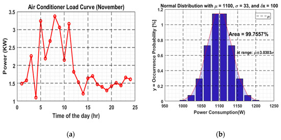
Figure 1. (a) Air conditioner load profile (November); (b) Distribution data with standard deviation of 33.

2.1.1. Off Load Method

The margin for deviation described above is quite narrow. For higher standard deviation, i.e., to allow wider spread in the distribution, it may be assumed that BBs supplied by a particular SST are not using air-conditioners at the specific time—which definitely presents a realistic picture as it is quite probable that a load is ON in some BBs and OFF in other BBs. Following mathematics is developed to analyze the scenario.

The existing mean power value of load at time t₁ is given as:

$$u_i(t_1)=x_i(t_1)$$

(1)

Provided the limits:

$$x_{min-i}<x_{Li}(t_1)<x_{max-i}$$

where u_Li(t₁) represents the averaged value at t₁, $x_{Li}(t_1)$ represents the power consumption, $x_{min-i}$ represents the minimum power consumption of and $x_{min-i}$ represents instantaneous maximum power consumption of the i^th load.

For wider standard deviation value, the mean value should be increased to new mean value as indicated in (2):

$$N_{ON-i}(t_1)=m-b_i$$

(2)

where $N_{ON-i}(t_1)$ represents the number of BBs for which i^th load is at ON sate while m represents the total number of buildings against each SST and b_i represents the number of BBs in which i^th load is at OFF state.

The new mean value is depicted in (3) as

$$u_i^{\prime }(t_1)=\raisebox{1ex}{$u_i(t_1)$}\!\left/ \!\raisebox{-1ex}{$N_{ON-i}(t_1)$}\right.$$

(3)

By utilizing the normal distribution technique, the data will be distributed between the $N_{ON-i}(t_1)$ BBs.

2.1.2. On/Off Method for Fixed Category Load

This subsection explains the distribution of the loading of fixed loads in BBs. Since these loads are either ON or OFF at their rated and zero power, respectively, the mean power value of fixed load at time ‘t₁’ is presented in (4).

$$u_{Fi}(t_1)=x_{Fi}(t_1)$$

(4)

Provided the limits:

$$x_{Fi}(t_1)<x_{Fmax-i}$$

where u_F-i(t₁) denotes the power t₁ and $x_{Fmax-i}$ represents the rated value of the i^th load.

Total mean power consumption of i^th load for ‘m’ number of BBs against each SST can be calculated using (5):

$$x_{total mean-i}(t_1)=u_{F-i}(t_1)\times m$$

(5)

where $x_{total mean-Fi}(t_1)$ represents the total mean power consumption of i^th load for all BBs.

Hence, the number of buildings for which the i^th load is ON can be represented as (6):

$$N_{ON-Fi}(t_1)=\frac{x_{total mean-Fi}(t_1)}{x_{Fmax-i}}$$

(6)

where $N_{ON-Fi}(t_1)$ represents the number of BBs for where the ith load is ON.

2.2. Mathematical Modeling

In case of AC distribution system, the grid voltage is at primary distribution level, which is stepped down via ‘k’ number of transformers (XMFR) supplying power to ‘j’ number of buildings. Each building is subsequently connected to ‘i’ number of loads. Each house is equipped with rooftop solar panels, and loads are connected to the in-house bus according to their load categorization defined earlier.

Similarly, in case of DC distribution system, the grid is DC which is connected to solid state transformers (SSTs), and the in-house source bus is DC, as presented in Figure 2. The equations for calculating the system efficiency at given time “t₁” are taken from [57], which is the effort of two of current authors.

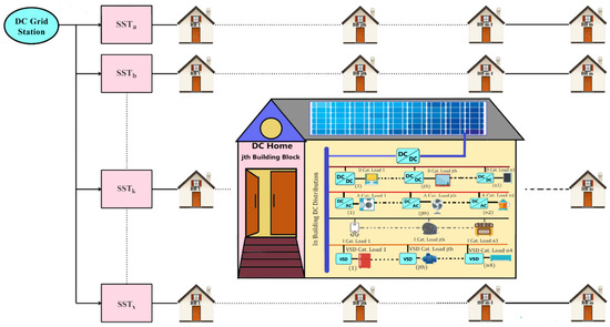
Figure 2. DC distribution System with load categorization.

2.2.1. DC System

For the total power consumption of a single BB (say j^th building), the input power p_j(t₁) may be calculated as the total sum of all four types of load categories at time t₁, as shown in (7)

$$p_j\left(t_1\right)=\left({\displaystyle \sum }_{i=1}^{n_1}{p}_{Dijk-in}\left(t_1\right)\right)+\left({\displaystyle \sum }_{i=1}^{n_2}{p}_{Aijk-in}\left(t_1\right)\right)+\left({\displaystyle \sum }_{i=1}^{n_3}{p}_{Iijk-in}\left(t_1\right)\right)+\left({\displaystyle \sum }_{i=1}^{n_4}{p}_{VSDijk-in}\left(t_1\right)\right)$$

(7)

where $p_j\left(t_1\right)$ is the input power demanded by the jth building block at time t₁; $p_{Dijk-in}\left(t_1\right)$, $p_{Aijk-in}\left(t_1\right)$, $p_{Iijk-in}\left(t_1\right)$ and $p_{VSDijk-in}\left(t_1\right)$ are the ith DC, AC, independent and VSD input powers in jth building block of kth SST, respectively. Normalized load data obtained by the process explained in Section 2.1 is used for the loads in Equation (1) with realistic load ratings from manufacturer’s data (given in Table 3). The appliance rating load matrix for DC loads is presented as:

$${\mathrm{Rating}}_{\mathrm{DC}\_\mathrm{loads}}=\left[\begin{array}{ccc}13 \mathrm{W}& 120 \mathrm{W}& 250 \mathrm{W}\\ 250 \mathrm{W}& 13 \mathrm{W}& 120 \mathrm{W}\\ 120 \mathrm{W}& 250 \mathrm{W}& 13 \mathrm{W}\end{array}\right]$$

(8)

Similar rating matrix for other load categories may be constructed by using Table 4. DC–DC, AC–DC, DC–AC, and VSD PECs are chosen based on their corresponding rating matrices with 10% oversize ratio. Since PEC efficiency varies with respect to the loading, therefore, the PEC curve equations (from loading-efficiency curves) are obtained using GRABIT tool using MATLAB, and efficiency equation for one of the DC/DC converter is presented in (9).

$${\eta }_{dd-ijk}\left(t_1\right)=-41.4 \times (p_{Dijk}\left(t_1\right)/ r_{ddijk}{)}^4+360.4 \times (p_{Dijk}\left(t_1\right)/ r_{ddijk}{)}^3 - 335.8 \times (p_{Dijk}\left(t_1\right)/ r_{ddijk}{)}^2 + 134.4 \times (p_{Dijk}\left(t_1\right)/ r_{ddijk})+74.83$$

(9)

where ${\eta }_{dd-ijk}$ is the efficiency of DC–DC converter for each ith load category in jth building block of kth SST. The DC efficiency matrix is obtained for other DC loads as well. Similar technique is employed for other load categories.

Table 4. Required PEC Rating for Each Residential Load.

Serial No.	Appliances	Category	Required PEC Ratings (Maximum)	PEC for DC System	PEC for AC System
1	Indoor Lights	D	300 W	DC/DC	AC/DC
2	Television	D	150 W	DC/DC	AC/DC
3	Computer	D	300 W	DC/DC	AC/DC
4	Dishwasher	A	1700 W	DC/AC	N/A
5	Clothe Dryer	A	5000 W	DC/AC	N/A
6	Clothe Washer	A	600 W	DC/AC	N/A
7	Air Conditioner	VSD	8000 W	DC/AC	VSD
8	Refrigerator	VSD	300 W	DC/AC	VSD

Since each building block is installed with a solar PV system whose PV curve equation is obtained through same procedure of curve fitting and is presented mathematically in (10)

$$p_{solar-j}\left(t_1\right)=\left\{{\lambda }_{SD-j}\times \left[{\alpha }_j{(t_1)}^4+{\beta }_j{(t_1)}^3+{\gamma }_j{(t_1)}^2+{\delta }_j\left(t_1\right)+{\epsilon }_j\left(t_1\right)\right]\right\}$$

(10)

where $p_{solar-j}\left(t_1\right)$ is the output power of solar system installed in jth building at time t₁ and ${\lambda }_{SD-j}$ is the associated DC–DC conversion loss. ${\alpha }_j, {\beta }_j, {\gamma }_j, {\delta }_j, {\epsilon }_j$ are the co-efficiencies obtained through curve fitting tool. ${\lambda }_{SD-j}$ is assumed to be constant for different power generation because this loss has negligible effect on system efficiency. It is also assumed that each building has same PV generation capacity; hence, the equation for PV system in all BBs is same. Subsequently, the input power drawn (or output power supplied in case of excess generation) by the system SST can be evaluated from (11):

$$p_{in-SSTa}\left(t_1\right)=\frac{p_{out-SSTa}\left(t_1\right)}{{\eta }_{SSTa}\left(t_1\right)}$$

(11)

$${\eta }_{ DC System}\left(t_1\right)=\left(\frac{p_{Load-total}\left(t_1\right)}{p_{DG}\left(t_1\right)+p_{solar-total}\left(t_1\right)}\right)$$

(12)

where $p_{DG}\left(t_1\right)$ is the required power from the DC grid at time t₁, which is calculated by summing the input power of each SST.${\eta }_{DC System}\left(t_1\right)$ is the efficiency of DC system, which is calculated by the dividing the sum of grid power $p_{DG}\left(t_1\right)$ and the total solar power $p_{solar-total}\left(t_1\right)$ to the total load power $p_{Load-total}\left(t_1\right)$ at time t₁, and $p_{Load-total}\left(t_1\right)$ is the total load power obtained by the summation of the power of each load category present in each building of each SST at time t₁.

2.2.2. AC System

Continuing the system modeling on similar lines as for the DC system, the AC system model is presented in Figure 3.

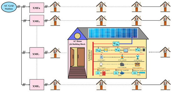
Figure 3. AC distribution System with load categorization.

The total load power for jth building is expressed in (13).

$$p_j\left(t_1\right)+q_j\left(t_1\right)=\left({\displaystyle \sum }_{i=1}^{n_1}{p}_{Dijk-in}\left(t_1\right)\right)+\left({\displaystyle \sum }_{i=1}^{n_2}\left(p_{Aijk-in}\left(t_1\right)+q_{Aijk-in}\left(t_1\right)\right)\right)+\left({\displaystyle \sum }_{i=1}^{n_3}{p}_{Iijk-in}\left(t_1\right)\right)+\left({\displaystyle \sum }_{i=1}^{n_4}{p}_{VSDijk-in}\left(t_1\right)\right)$$

(13)

where $p_j\left(t_1\right)$ and $q_j\left(t_1\right)$ are the required powers of jth building while $p_{Dijk-in}\left(t_1\right)$, $p_{Aijk-in}\left(t_1\right)q\left(t_1\right)$, $p_{Iijk-in}\left(t_1\right)$ and $p_{VSDijk-in}\left(t_1\right)$ represent the ith DC, AC, independent, and VSD input powers in jth building block of k^th XMFR, respectively. Similar procedure is performed for rating and efficiency matrices in AC system using curve fitting tool.

The solar power generated by jth building in the AC system is expressed mathematically in (14):

$$p_{solar-j}\left(t_1\right)=\left\{{\lambda }_{SA-j}\times \left[{\alpha }_j{(t_1)}^4+{\beta }_j{(t_1)}^3+{\gamma }_j{(t_1)}^2+{\delta }_j\left(t_1\right)+{\epsilon }_j\left(t_1\right)\right]\right\}$$

(14)

where ${\lambda }_{SA-j}$ represents DC–AC inverter losses associated with solar system installed in j^th building. Similar to the case of DC, ${\lambda }_{SA-j}$ is assumed constant. The consideration of the reactive component is presented in (15).

$$q_{sola{r}_j}\left(t_1\right)=\mu \times p_{sola{r}_j}\left(t_1\right)$$

(15)

where, $q_{solar-j}\left(t_1\right)$ is reactive output power of solar system delivered to each building, while the reactive power supplied by the solar inverters is treated as a fractional factor μ of the real power. The difference compared to the DC model is the use of λ_SA variable, which represents solar to AC power conversion.

The power drawn by the distribution transformer S_in-XMFR, can be evaluated using (16):

$$\begin{gathered} \left|S_{i{n}_{Xfmr}}\left(t_1\right)\right|=\frac{{{\displaystyle \sum }}_{j=1}^m\left(\left|p_{demand-j}\left(t_1\right)+j{q}_{demand-j}\left(t_1\right)\right|\right)}{{\eta }_{xmfr}\left(t_1\right)} \\ <S_{i{n}_{Xfmr}}\left(t_1\right)={tan}^{-1}\frac{p_{demand-j}\left(t_1\right)}{q_{demand-j}\left(t_1\right)} \end{gathered}$$

(16)

where,

$$\begin{gathered} p_{demand-j}\left(t_1\right)={\displaystyle \sum }_{j=1}^m\left[\left(p_j\left(t_1\right)+p_{solar-j}(t_1)\right)\right] \\ {q}_{demand-j}\left(t_1\right)={\displaystyle \sum }_{j=1}^m\left[\left(q_j\left(t_1\right)+q_{solar-j}(t_1)\right)\right] \end{gathered}$$

where $S_{in-Xfmr}(t_1)$ is complex power available at input side of the transformer, which is calculated by the sum of real power demand $p_{demand-j}\left(t_1\right)$ and reactive power demand $q_{demand-j}\left(t_1\right)$; by utilizing the transformer efficiency ${\eta }_{xmfr}\left(t_1\right)$ at time t₁

The system efficiency values can be determined using (17):

$${\eta }_{ AC System}\left(t_1\right)=\left(\frac{p_{Load-total}\left(t_1\right)}{p_{AG}\left(t_1\right)+p_{solar-total}\left(t_1\right)}\right)$$

(17)

where ${\eta }_{AC System}\left(t_1\right)$ is the efficiency of AC system, which is calculated by the dividing the sum of grid power $p_{AG}\left(t_1\right)$ and real solar power $p_{solar-total}\left(t_1\right)$ to the total load power $p_{Load-total}\left(t_1\right)$ at time t₁.

A single BB is designed and simulated in MATLAB/Simulink environment. A total of 27 residential BBs (9 buildings per phase, giving a total of 27 for the three-phase system) are assumed to be combined and connected with a single distribution transformer. For the DC distribution system, this transformer is replaced with a DC–DC PEC SST. In the secondary DC system, the voltage level of 326 V (peak of 230 V_rms AC) is chosen, which draws its support from [33].

2.3. Sensitivity Analysis

The basic purpose of the sensitivity analysis is to evaluate the effect of variation in the individual load type PEC efficiency, main grid tie PEC efficiency, and PV system capacity on overall the system’s efficiency. Following mathematical model is devised for studying the effect of the efficiency variation of each component in DC system. Similar process shall be adopted with the AC system.

2.3.1. PV Capacity Variation

The generalized equation of p_solar−j for jth building is given in (18):

$$p_{solar-j}\left(t_1\right)=\left\{{\lambda }_j\times C\mathrm{s}\times \left[{\alpha }_j{\left(t_1\right)}^4+{\beta }_j{\left(t_1\right)}^3+{\gamma }_j{\left(t_1\right)}^2+{\delta }_j\left(t_1\right)+{\epsilon }_j\right]\right\}$$

(18)

where ${\lambda }_j$ is the associated PEC efficiency factor and Cs is the installed PV capacity in j^th BB. The installed capacity is varied to see the effect of PV capacity on overall system efficiency. For this purpose, Cs is considered 1pu (normalized form), and variable ‘x’ is taken as scaling factor for capacity; thereby, (18) takes the form of (19) and (20).

$$p_{solar-j}{\left(t_1\right)}^{\prime }=\left\{{\lambda }_j\times C\mathrm{s} \times x\times \left[{\alpha }_j{\left(t_1\right)}^4+{\beta }_j{\left(t_1\right)}^3+{\gamma }_j{\left(t_1\right)}^2+{\delta }_j\left(t_1\right)+{\epsilon }_j\right]\right\}$$

(19)

$$p_{solar-j}{\left(t_1\right)}^{\prime }=p_{solar-j}\left(t_1\right)\times x$$

(20)

for x = 1

$$p_{solar-j}{\left(t_1\right)}^{\prime }=p_{solar-j}\left(t_1\right)$$

for x > 1

$$p_{solar-j}{\left(t_1\right)}^{\prime }>p_{solar-j}\left(t_1\right)$$

for 0 < x < 1

$$p_{solar-j}{\left(t_1\right)}^{\prime }<p_{solar-j}\left(t_1\right)$$

and the rest of mathematical model takes the form, as shown in (21) to (25):

$$p_{demand-j}{\left(t_1\right)}^{\prime }=p_j\left(t_1\right)-p_{solar-j}{\left(t_1\right)}^{\prime }$$

(21)

$$p_{out-SSTa}{\left(t_1\right)}^{\prime }=\left({\displaystyle \sum }_{j=1}^m{p}_{demand-j}\left(t_1\right)\prime \right)$$

(22)

$$p_{demand-j}{\left(t_1\right)}^{\prime }=p_j\left(t_1\right)-p_{solar-j}{\left(t_1\right)}^{\prime }$$

(23)

$$p_{out-SSTa}{\left(t_1\right)}^{\prime }=\left({\displaystyle \sum }_{j=1}^m{p}_{demand-j}\left(t_1\right)\prime \right)$$

(24)

$${\eta }_{ DC System}{\left(t_1\right)}^{\prime }=\left(\frac{p_{out}\left(t_1\right)}{p_{in}\left(t_1\right)}\right)=\left(\frac{p_{Load-total}\left(t_1\right)}{p_{DG}\left(t1\right)+p_{solar-total}\left(t_1\right)\prime }\right)$$

(25)

2.3.2. PEC Efficiency Variation

The generalized PEC curve equation in both distribution systems is presented in (26)

$${\eta }_{PEC-ijk}\left(t_1\right)=a_{ijk}{\left(\frac{p_{ijk}\left(t_1\right)}{r_{PECijk}}\right)}^4+b_{ijk}{(\dots )}^3{c}_{ijk}{(\dots )}^2+d_{ijk}(\dots )+e_{ijk}$$

(26)

In order to observe the effect of varying efficiency of PEC, a factor is required which can decrease or increase the efficiency of PEC at any given time t₁ from its original value.

Let that factor be a constant shift “K”, mathematically presented in (27) and (28)

$${\eta }_{PEC-ijk}{\left(t_1\right)}^{\prime }=a_{ijk}{\left(\frac{p_{ijk}\left(t_1\right)}{r_{PECijk}}\right)}^4+b_{ijk}{(\dots )}^3+c_{ijk}{(\dots )}^2+d_{ijk}(\dots )+e_{ijk}+K$$

(27)

$${\eta }_{PEC-ijk}{\left(t_1\right)}^{\prime }={\eta }_{PEC-ijk}\left(t_1\right)+K$$

(28)

Since the overall system efficiency is indirectly related to efficiency curve of PEC, hence the mathematical model is maneuvered accordingly in (29) to (36).

$$p_j{\left(t_1\right)}^{}=\left({\displaystyle \sum }_{i=1}^{n_1}\frac{p_{D-ijk}\left(t_1\right)}{{\eta }_{dd-ijk}\left(t_1\right)}\right)+\left({\displaystyle \sum }_{i=1}^{n_2}\frac{p_{A-ijk}\left(t_1\right)}{{\eta }_{da-ijk}\left(t_1\right)}\right)+\left({\displaystyle \sum }_{i=1}^{n_2}\frac{p_{VSD-ijk}\left(t_1\right)}{{\eta }_{vsd-ijk}\left(t_1\right)}\right)+\left({\displaystyle \sum }_{i=1}^{n_3}{p}_{I-ijk}\left(t_1\right)\right)$$

(29)

$${\eta }_{PEC}^{\prime }={\eta }_{PEC}+K$$

(30)

In order to achieve variation, the K factor is added into ${\eta }_{dd}$,${\eta }_{da}$,${\eta }_{vsd}, {\eta }_{SST}$ to assess the effect of variation in the PEC efficiency. Utilizing (29) for ${\eta }_{PEC}^{\prime }$

$$p_j{\left(t_1\right)}^{\prime }=\left({\displaystyle \sum }_{i=1}^{n_1}\frac{p_{D-ijk}\left(t_1\right)}{{\eta }_{dd-ijk}\left(t_1\right)\prime }\right)+\left({\displaystyle \sum }_{i=1}^{n_2}\frac{p_{A-ijk}\left(t_1\right)}{{\eta }_{da-ijk}\left(t_1\right)\prime }\right)+\left({\displaystyle \sum }_{i=1}^{n_2}\frac{p_{VSD-ijk}\left(t_1\right)}{{\eta }_{vsd-ijk}\left(t_1\right)\prime }\right)+\left({\displaystyle \sum }_{i=1}^{n_3}{p}_{I-ijk}\left(t_1\right)\right)$$

(31)

$$p_{demand-j}{\left(t_1\right)}^{\prime }=p_j{\left(t_1\right)}^{\prime }-p_{solar-j}\left(t_1\right)$$

(32)

$$p_{out-SSTa}{\left(t_1\right)}^{\prime }=\left({\displaystyle \sum }_{j=1}^m{p}_{demand-j}\left(t_1\right)\prime \right)$$

(33)

$$p_{in-SSTa}{\left(t_1\right)}^{\prime }=\frac{p_{out-SSTa}\left(t_1\right)\prime }{{\eta }_{SSTa}\left(t_1\right)\prime }$$

(34)

$$p_{DG}{\left(t_1\right)}^{\prime }={\displaystyle \sum }_{k=a}^x{p}_{in-SSTa}\left(t_1\right)\prime$$

(35)

$${\eta }_{ DC System}{\left(t_1\right)}^{\prime }=\left(\frac{p_{out}\left(t_1\right)}{p_{in}\left(t_1\right)}\right)=\left(\frac{p_{Load-total}\left(t_1\right)}{p_{DG}\left(t_1\right)\prime +p_{solar-total}\left(t_1\right)}\right)$$

(36)

Similar approach is developed for AC system by making appropriate changes in Equation (27).

3. Main Results

For the comparison of AC and DC systems, this paper focused mainly on efficiency factors for different sets of scenarios such as weekends and weekdays for seasonal and hourly load profiles and variations in PEC efficiencies.

3.1. Structural Visualization of Scenarios in Both Systems

Figure 4 and Figure 5 demonstrate structural visualization of the scenarios on both systems. The hourly load profile is extracted from [34] for both weekdays and weekends of various months in order to achieve diversity. After normalizing the load data, the efficiency analysis was performed for both systems using computer software MATLAB in accordance with the mathematical equations presented in Section 2.

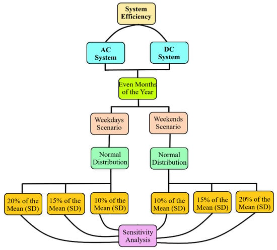
Figure 4. Combined AC and DC Systems Analysis.

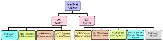
Figure 5. The Flow of Sensitivity Analysis.

3.2. Comparative Efficiency Analysis of Both Systems

Following are the results for comparative efficiency analysis with normalized data and without any variation of other parameters such as PEC efficiency or PV capacity. The base value of PV capacity is chosen to be 1000 W, installed on each BB. Figure 6 shows the result of the comparative analysis for six months with 10%, 15%, and 20% standard deviation percentages for the AC and DC systems, respectively.

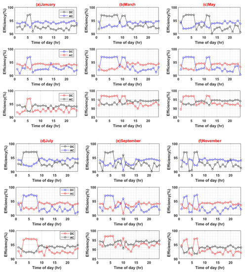
Figure 6. Efficiency analyses of AC and DC System (Weekdays).

The maximum efficiency values for the AC system are 96.82%, 96.87%, and 96.8%, at a standard deviation of 10%, 15%, and 20%, respectively. Similarly, the maximum efficiency values for the DC system are 97.63%, 97.58%, and 97.72%, at a standard deviation of 10%, 15%, and 20%, respectively. Hence, in the base case scenario, the DC system possesses a minute efficiency advantage over the AC system (see Figure 7).

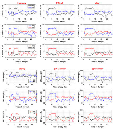
Figure 7. Efficiency analyses of AC and DC System (Weekends).

3.3. Comparative Sensitivity Analysis on Both Systems

Figure 8 and Figure 9 present the results of main XFMR and main SST efficiency variation for the AC and DC systems, respectively, incorporating a variation of −10% to 1%. The upper limit of 1% draws support from the fact that the main PEC’s maximum efficiency gain for the selected PEC cannot exceed 1% at the rated load.

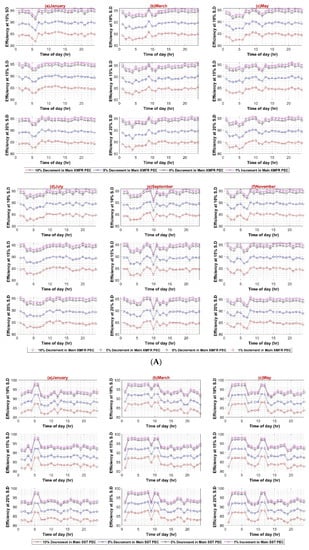
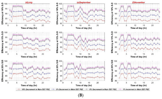
Figure 8. AC System efficiency with respect to XFMR efficiency variation (A) Weekdays; (B) Weekend.

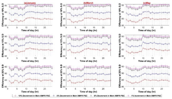
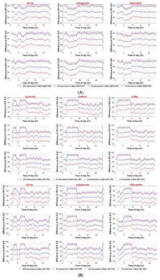
Figure 9. DC System efficiency with respect to XFMR efficiency variation (A) Weekdays; (B) Weekend.

The results depict the AC system efficiency varying between 81% and 96% for weekdays, whereas, for weekends, the efficiency variation is between 81% and 97%.

Similarly, the maximum system efficiency in the DC system is 98.5%, whereas the minimum efficiency value is 80% during the weekday scenario. The maximum and minimum efficiency values for weekends are 98% and 80%, respectively. The results depict strong dependence of systems efficiencies on main converters, i.e., transformer in AC case and SST in DC case. The reason for the direct dependence of the efficiency values on main converters lies in the fact that bulk power transfers from these converters to the rest of the system up to the load end. The higher efficiency of these converters presents overall lower losses and improves overall system efficiency. The effect of each of the in-house PEC efficiency variations is shown in Appendix A.

3.4. Discussion

This work aims to assist and inform an industry decision on whether to adopt DC power distribution in residential buildings or not. In comparison to previous research efforts, this work employs detailed mathematical modeling-based implementation to compare equivalent AC and DC residential building distribution networks powered through utility as well as a renewable energy source (RES). The electrical building models are composed of realistic load profiles and converter efficiency curves based on market data. The findings of this study are helpful in making a conclusion about the current position of AC and DC distribution systems and how it may change in the future with the improvement of technology in the future.

This research found that the baseline efficiency saving in the case of the DC distribution system is about 2% to 3% during the period of the day. The efficiency of the DC distribution system was found to be much better with larger solar PV capacity. In the practical world, where the load is always unpredictable and RER generation is stochastic in nature, extreme component condition variations are incorporated, i.e., variation of standard deviation ranging from 5% to 20% of mean load value, solar PV capacity variation between 1000 W to 9000 W and variation in PEC efficiencies for the sake of a fair comparison between both systems to make the system realistic as much as possible.

In the first case scenario, the efficiency of AC–DC PEC for inheriting the DC load in an AC system is varied from a 10% decrement to a 5% increment in a step of 5% to evaluate any possible effect on the whole AC system efficiency for 10%, 15% and 20% standard deviation of load, respectively for both weekdays and weekends. This is to account for future PEC technologies growth and higher penetration of inherited DC loads. The results in Figure A1A,B show an insignificant 0.8% decrease in overall system efficiency for weekdays, and for weekends, it is less than 0.5%. This is due to the reason that at each individual load, the AC–DC converter is already operating close to its nominal ratings, and, in comparison to the main XFMR, a very small current pass through it. Hence system loss is much smaller, and system efficiency is not notably affected.

In the second scenario, the efficiency of VSD in the AC system varied from 10% to 1% increments in steps of 5%. The mere 1% increment increase is due to the fact that the currently available VSD converter was already reaching efficiencies close to 100%. Therefore, a further increment was not needed here. Similar to the first case, the standard deviation of the load varied from 10% to 20% for both weekdays and weekends. Figure A2A,B shows a significant effect of VSD efficiency variation on AC system efficiency, in some months reaching as high as 13% for both weekdays and weekends. This was to be expected as most of the VSD loads are high-powered loads that draw extensive amounts of current. With as high as 20% load variation, this effect becomes more evident as a higher number of currents causes greater heat losses.

In the third case, PV capacity size is varied to evaluate the impact of higher onsite RER power injection into the AC system in the range of 1 kW to 9 kW in four equal intervals for 10%, 15%, and 20% standard deviation of load, respectively for both weekdays and weekends. It can be observed from Figure A3A,B that increasing the PV capacity has a notable effect on AC system efficiency as more power is readily available onsite. Hence less power is required from the utility, and ultimately less power flows through the main XFMR, and fewer transmission losses are incurred. Thus, the efficiency of the system increases with PV capacity. It can also be perceived from the weekend results that system efficiency is much lower at the start of the day as compared to weekdays. This can be attributed to the fact that load demand is reduced, and the main XFMR operates under nominal ratings and shows low efficiency at reduced loading.

Similar to AC systems, all case scenarios are performed for DC–DC, DC–AC, VFD PEC, and PV capacity for the DC system. As expected in the case of the DC–DC converter, system efficiency remains insensitive to the DC–DC converter efficiency variations because of the same reason as AC–DC for very low DC load. In the case of DC–AC efficiency variation, DC system efficiency is noticeably affected by it, ranging from 4% to 6% on weekdays and weekends, respectively, as shown in Figure A5A,B. For VFD loads, variation in efficiencies of VFD converters had a significant effect on DC system efficiency as VFD PEC is used for high power loads. Since VFD PEC is a two-stage converter in which first DC voltage is shifted to the required voltage level and then transformed into desired AC voltage for VFD loads. Thus, this two-stage conversion leads to higher efficiency losses. However, VFD PEC in the DC system is more efficient in comparison to VFD converters in the AC system because of the AC–DC rectifiers that are used in the first stage, which results in high power loss as compared to the DC–DC stage. The efficiency variation in VFD converters for the DC system varied between 7% and 8% in the worst case for weekdays and weekends, respectively, as shown in Figure A6A,B. In the last case for variations in PV capacity size, it had very little effect, roughly less than 3% variation in DC system efficiency in comparison to AC system, as shown in Figure A7A,B.

4. Conclusions and Future Recommendations

It can be concluded that the efficiency of the main PEC plays a major role in the superiority decision of one system over the other. In the authors’ opinion, since the transformer design field is well saturated already and its efficiency improvement is at its pinnacle; hence, further improvement in its efficiency may not occur soon in the future with the current technology. However, there is still room for improvement in the SST converters as regards efficiency, resulting in further enhancement in DC system efficiency. The current effort establishes a baseline for efficiency dominancy with DC; other factors which affect the system’s efficiency must be examined in order to reach a concrete decision. After performing the sensitivity analysis, the results of both AC and DC systems for all case scenarios are compared. It is evident that maximum system efficiency variation occurs with variation in main converter efficiency, and minimum system efficiency variation occurs with variation in solar PV capacity. The effect of variation in load end PECs is intermediate between that of main converters and solar PV capacity. The baseline efficiency advantage of 2% to 3% during the day exists for the case of the DC distribution system as compared to the AC distribution system.

For future work, the analyses of this work might be performed for different voltage levels for BB bus and with the respective voltage level PECs. Our analysis was based on 230 V AC. Ultimately, a comprehensive techno-economic analysis is required to thoroughly measure the savings of DC distribution and the decision that: are the savings obtained enough to justify the replacement of the AC system.

In summarizing, the current effort has attempted to highlight the shortcomings in the area of DC distribution efficiency analyses and has also attempted to partly fill in this gap by providing a variety of simulation studies comprising many comparative (AC vs. DC) sensitivity analyses. Nevertheless, limitations exist in this work, such as expanding averaged data to instantaneous data—a better option is to use actual instantaneous data of each individual load in a locality. Similarly, using a specific set of ratings of different loads can also is a limitation—a real-life-based wider set can yield closer to actual results. Future efforts in this direction can take guidance from the approach of the current work and try to overcome the shortcomings of this work as well as expand the scenarios presented in the current study.

References

- Sulzberger, C.L. Triumph of ac-from Pearl Street to Niagara. IEEE Power Energy Mag. 2003, 1, 64–67. [Google Scholar] [CrossRef]
- McPherson, S.S. War of the Currents: Thomas Edison vs. Nikola Tesla; Twenty-First Century Books: Chicago, IL, USA, 2012. [Google Scholar]
- Allerhand, A. A contrarian history of early electric power distribution [scanning our past]. In Proceeding of the IEEE; IEEE: Piscataway, NJ, USA, 2017; Volume 105, pp. 768–778. [Google Scholar]
- McNichol, T. AC/DC: The Savage Tale of the First Standards War; John Wiley & Sons: Hoboken, NJ, USA, 2011. [Google Scholar]
- Fairley, P. DC versus AC: The second war of currents has already begun [in my view]. IEEE Power Energy Mag. 2012, 10, 103–104. [Google Scholar] [CrossRef]
- Dastgeer, F.; Gelani, H.E.; Anees, H.M.; Paracha, Z.J.; Kalam, A. Analyses of efficiency/energy-savings of DC power distribution systems/microgrids: Past, present and future. Int. J. Electr. Power Energy Syst. 2019, 104, 89–100. [Google Scholar] [CrossRef]
- Capasso, C.; Rubino, G.; Rubino, L.; Veneri, O. Power architectures for the integration of photovoltaic generation systems in DC-microgrids. Energy Procedia 2019, 159, 34–41. [Google Scholar] [CrossRef]
- Musasa, K.; Nwulu, N.I.; Gitau, M.N.; Bansal, R.C. Review on DC collection grids for offshore wind farms with high-voltage DC transmission system. IET Power Electron. 2017, 10, 2104–2115. [Google Scholar] [CrossRef]
- Singh, M.; Khadkikar, V.; Chandra, A.; Varma, R.K. Grid interconnection of renewable energy sources at the distribution level with power-quality improvement features. IEEE Trans. Power Deliv. 2010, 26, 307–315. [Google Scholar] [CrossRef]
- Owusu, P.A.; Sarkodie, S. A review of renewable energy sources, sustainability issues and climate change mitigation. Cogent Eng. 2016, 3, 1167990. [Google Scholar] [CrossRef]
- Alassi, A.; Bañales, S.; Ellabban, O.; Adam, G.; MacIver, C. HVDC transmission: Technology review, market trends and future outlook. Renew. Sustain. Energy Rev. 2019, 112, 530–554. [Google Scholar] [CrossRef]
- Shinde, M.P.; Helonde, J.B. An Overview of HVDC Power Transmission System with Voltage Source Converter. Int. J. Recent Innov. Trends Comput. Commun. 2018, 6, 240–244. [Google Scholar]
- Gerber, D.L.; Liou, R.; Brown, R. Energy-saving opportunities of direct-DC loads in buildings. Appl. Energy 2019, 248, 274–287. [Google Scholar] [CrossRef]
- Thomas, B.A. Edison revisited: Impact of DC distribution on the cost of LED lighting and distributed generation. In Proceedings of the 2010 Twenty-Fifth Annual IEEE Applied Power Electronics Conference and Exposition (APEC), Palm Springs, CA, USA, 21–25 February 2010; IEEE: Piscataway, NJ, USA, 2010. [Google Scholar]
- Rathikrindi, K.S.; Paramasivam, S.; Sandeep, L. Energy saving opportunities through variable frequency drive for commercial air conditioners. In Proceedings of the 2018 4th International Conference on Electrical Energy Systems (ICEES), Chennai, India, 7–9 February 2018; IEEE: Piscataway, NJ, USA, 2018. [Google Scholar]
- Kamran, M.; Bilal, M.; Mudassar, M. DC home appliances for DC distribution system. Mehran Univ. Res. J. Eng. Technol. 2017, 36, 881–890. [Google Scholar] [CrossRef]
- NakuÃ, L.; Spahiu, A. Saving energy by replacing IM with BLDC MOTOR in fan application. Eur. J. Electr. Eng. Comput. Sci. 2018, 2. [Google Scholar] [CrossRef]
- Brenguier, J.; Vallet, M.; Vaillant, F. Efficiency gap between AC and DC electrical power distribution system. In Proceedings of the 2016 IEEE/IAS 52nd Industrial and Commercial Power Systems Technical Conference (I&CPS), Detroit, MI, USA, 1–5 May 2016; IEEE: Piscataway, NJ, USA, 2016. [Google Scholar]
- Fregosi, D.; Ravula, S.; Brhlik, D.; Saussele, J.; Frank, S.; Bonnema, E.; Scheib, J.; Wilson, E. A comparative study of DC and AC microgrids in commercial buildings across different climates and operating profiles. In Proceedings of the 2015 IEEE First International Conference on DC Microgrids (ICDCM), Atlanta, GA, USA, 7–10 June 2015; IEEE: Piscataway, NJ, USA, 2015. [Google Scholar]
- Gerber, D.L.; Vossos, V.; Feng, W.; Marnay, C.; Nordman, B.; Brown, R. A simulation-based efficiency comparison of AC and DC power distribution networks in commercial buildings. Appl. Energy 2018, 210, 1167–1187. [Google Scholar] [CrossRef]
- Manandhar, U.; Ukil, A.; Jonathan, T.K.K. Efficiency comparison of DC and AC microgrid. In Proceedings of the 2015 IEEE Innovative Smart Grid Technologies-Asia (ISGT ASIA), Bangkok, Thailand, 3–6 November 2015; IEEE: Piscataway, NJ, USA, 2016. [Google Scholar]
- Siraj, K.; Khan, H.A. Dc distribution for residential power networks—A framework to analyze the impact of voltage levels on energy efficiency. Energy Rep. 2020, 6, 944–951. [Google Scholar] [CrossRef]
- Atia, H.R.; Shakya, A.; Tandukar, P.; Tamrakar, U.; Hansen, T.M.; Tonkoski, R. Efficiency analysis of AC coupled and DC coupled microgrids considering load profile variations. In Proceedings of the 2016 IEEE International Conference on Electro Information Technology (EIT), Grand Forks, ND, USA, 19–21 May 2016; IEEE: Piscataway, NJ, USA, 2016. [Google Scholar]
- Sirsi, R.; Prasad, S.; Sonawane, A.; Lokhande, A. Efficiency comparison of AC distribution system and DC distribution system in microgrid. In Proceedings of the 2016 International Conference on Energy Efficient Technologies for Sustainability (ICEETS), Nagercoil, India, 7–8 April 2016; IEEE: Piscataway, NJ, USA, 2016. [Google Scholar]
- Vossos, V.; Garbesi, K.; Shen, H. Energy savings from direct-DC in US residential buildings. Energy Build. 2014, 68, 223–231. [Google Scholar] [CrossRef]
- Boeke, U.; Wendt, M. DC power grids for buildings. In Proceedings of the 2015 IEEE First International Conference on DC Microgrids (ICDCM), Atlanta, GA, USA, 7–10 June 2015; IEEE: Piscataway, NJ, USA, 2015. [Google Scholar]
- Weiss, R.; Ott, L.; Boeke, U. Energy efficient low-voltage DC-grids for commercial buildings. In Proceedings of the 2015 IEEE First International Conference on DC Microgrids (ICDCM), Atlanta, GA, USA, 7–10 June 2015; IEEE: Piscataway, NJ, USA, 2015. [Google Scholar]
- Viitanen, J.; Halonen, L. Electrical efficiency study of alternating current and direct current power topologies in office building with integrated photovoltaics in Matlab-Simulink environment. J. Renew. Sustain. Energy 2014, 6, 033123. [Google Scholar] [CrossRef]
- Hammerstrom, D.J. AC versus DC distribution systemsdid we get it right? In Proceedings of the 2007 IEEE Power Engineering Society General Meeting, Tampa, FL, USA, 24–28 June 2007; IEEE: Piscataway, NJ, USA, 2007. [Google Scholar]
- Nilsson, D.; Sannino, A. Efficiency analysis of low-and medium-voltage DC distribution systems. In Proceedings of the IEEE Power Engineering Society General Meeting, Denver, CO, USA, 6–10 June 2004; IEEE: Piscataway, NJ, USA, 2005. [Google Scholar]
- Montoya, O.D.; Serra, F.M.; De Angelo, C.H. On the efficiency in electrical networks with ac and dc operation technologies: A comparative study at the distribution stage. Electronics 2020, 9, 1352. [Google Scholar] [CrossRef]
- Ahmad, F.; Dastgeer, F.; Gelani, H.E.; Khan, S.; Nasir, M. Comparative Analyses of Residential Building Efficiency for AC and DC Distribution Networks. Bull. Pol. Acad. Sci. Tech. Sci. 2021, 69, e136732. [Google Scholar]
- Dastgeer, F.; Gelani, H.E. A Comparative analysis of system efficiency for AC and DC residential power distribution paradigms. Energy Build. 2017, 138, 648–654. [Google Scholar] [CrossRef]
- Gelani, H.E.; Dastgeer, F.; Siraj, K.; Nasir, M.; Niazi, K.A.K.; Yang, Y. Efficiency comparison of AC and DC distribution networks for modern residential localities. Appl. Sci. 2019, 9, 582. [Google Scholar] [CrossRef]
- Gelani, H.E.; Dastgeer, F. Efficiency analyses of a DC residential power distribution system for the modern home. Adv. Electr. Comput. Eng. 2015, 15, 135–143. [Google Scholar] [CrossRef]
- Gelani, H.E.; Nasir, M.; Dastgeer, F.; Hussain, H. Efficiency comparison of alternating current (AC) and direct current (DC) distribution system at residential level with load characterization and daily load variation. Proc. Pak. Acad. Sci. A. Phys. Comput. Sci. 2017, 54, 111–118. [Google Scholar]
- Rasheed, A.; Khan, S.; Gelani, H.E.; Dastgeer, F. AC vs. DC Home: An Efficiency Comparison. In Proceedings of the 2019 International Symposium on Recent Advances in Electrical Engineering (RAEE), Islamabad, Pakistan, 28–29 August 2019; IEEE: Piscataway, NJ, USA, 2019. [Google Scholar]
- Glasgo, B.; Azevedo, I.L.; Hendrickson, C. How much electricity can we save by using direct current circuits in homes? Understanding the potential for electricity savings and assessing feasibility of a transition towards DC powered buildings. Appl. Energy 2016, 180, 66–75. [Google Scholar] [CrossRef]
- Electric Power Research Institute (EPRI). End Use Load Shapes Data. 2012–2013. Available online: https://loadshape.epri.com/enduse (accessed on 11 May 2022).
- Table 2—2015 Residential Energy End-Use Splits, by Fuel Type (QuadrillionBtu). Available online: http://buildingsdatabook.eren.doe.gov/TableView.aspx? (accessed on 11 May 2022).
- Instantaneous Power Consumption of Appliances. Available online: https://www.daftlogic.com/information-appliance-power-consumption.htm (accessed on 11 May 2022).
- How Much Power is Consumed by Computer. Available online: https://www.kompulsa.com/much-power-computers-consume/ (accessed on 11 May 2022).
- How Much Power Do Your Appliances Use? Available online: https://www.wholesalesolar.com/solar-information/power-table (accessed on 11 May 2022).
- Typical Power Rating of Common Electrical Equipment. Available online: https://www.sgs-engineering.com/help-advice/typical-power-ratings-of-common-electrical-equipment/ (accessed on 11 May 2022).
- RECOM RACG150-12S 150 W AC-DC Converter. Available online: https://recom-power.com/pdf/Powerline_AC-DC/RACG150.pdf (accessed on 11 May 2022).
- CUI INC PDRB-300-24 300 W AC-DC Converter. Available online: https://www.cui.com/product/internal-ac-dc-power-supplies/din-rail/pdrb-300-series (accessed on 11 May 2022).
- MORNINGSTAR SI-300-115V-UL SI-300-220 V 300 W DC-AC Inverter. Available online: https://ww.morningstarcorp.com/products/suresine/ (accessed on 11 May 2022).
- SUNGROW SG8K-D 8000 W DC/AC Inverter. Available online: https://ww.gemenergy.com.au/wp-content/uploads/2019/12/SG8K-D-Datasheet.pdf (accessed on 11 May 2022).
- CALEX 24S12.12QSW (ROHS) 150 W DC-DC Converter. Available online: http://calex.com/pdf/qsw.pdf (accessed on 11 May 2022).
- TOSHIBA RD024 300 W Isolated DC-DC Converter. Available online: https://toshiba.semicon-storage.com/ap-en/semiconductor/designdevelopment/referencedesign/articles/300w-Isolated-dc-dc_powermanagement_rd024.html (accessed on 11 May 2022).
- Texas Instruments 600 W DC-AC Inverter Reference Design. Available online: http://www.ti.com/tool/TIDM-HV-1PH-DCAC?keyMatch=TIDM-HV-1PH-DCAC&tisearch=Search-EN-everything&usecase=GPN#Technical%20Documents (accessed on 11 May 2022).
- SMA SB1700 1700 W DC-AC Inverter. Available online: https://www.eco-logisch.nl/pdfupload/SMA%20SB%201700.pdf (accessed on 11 May 2022).
- ABB String Inverter PVI-5000-TL-OUTD 5000 W DC-AC Inverter. Available online: https://library.e.abb.com/public/056a93c2644e4f15b55475647c6e0156/PVI-5000-ENRev%20E.pdf (accessed on 11 May 2022).
- Baldwin, T.L.; Turk, R.J.; Myers, K.S.; Gentle, J.P.; Bush, J.W. Transformer Efficiency Assessment—Okinawa, Japan; U.S. Department of Energy: Portland, OR, USA, 2012. [Google Scholar] [CrossRef]
- ApECOR 200 kW Bidirectional DC-DC. Available online: http://apecor.com/pages/products/highpower/apecor_ev_bidirectional_dcdc.pdf (accessed on 11 May 2022).
- Lukhwareni, T.; Dobzhanskyi, O.; Gouws, R. Solar power pumping system for domestic appliances. In Proceedings of the Twenty-Second Domestic Use of Energy, Cape Town, South Africa, 1–2 April 2014; pp. 1–6. [Google Scholar] [CrossRef]
- Dastgeer, F.; Anees, H.M.; Gelani, H.E.; Amjad, K.; Javeed, M.R. A basic mathematical testbed for energy efficiency analyses of DC power distribution systems/microgrids. Bull. Electr. Eng. Inform. 2021, 10, 1484–1494. [Google Scholar] [CrossRef]
Publisher’s Note: MDPI stays neutral with regard to jurisdictional claims in published maps and institutional affiliations. |
© 2022 by the authors. Licensee MDPI, Basel, Switzerland. This article is an open access article distributed under the terms and conditions of the Creative Commons Attribution (CC BY) license (https://creativecommons.org/licenses/by/4.0/).