1. Introduction
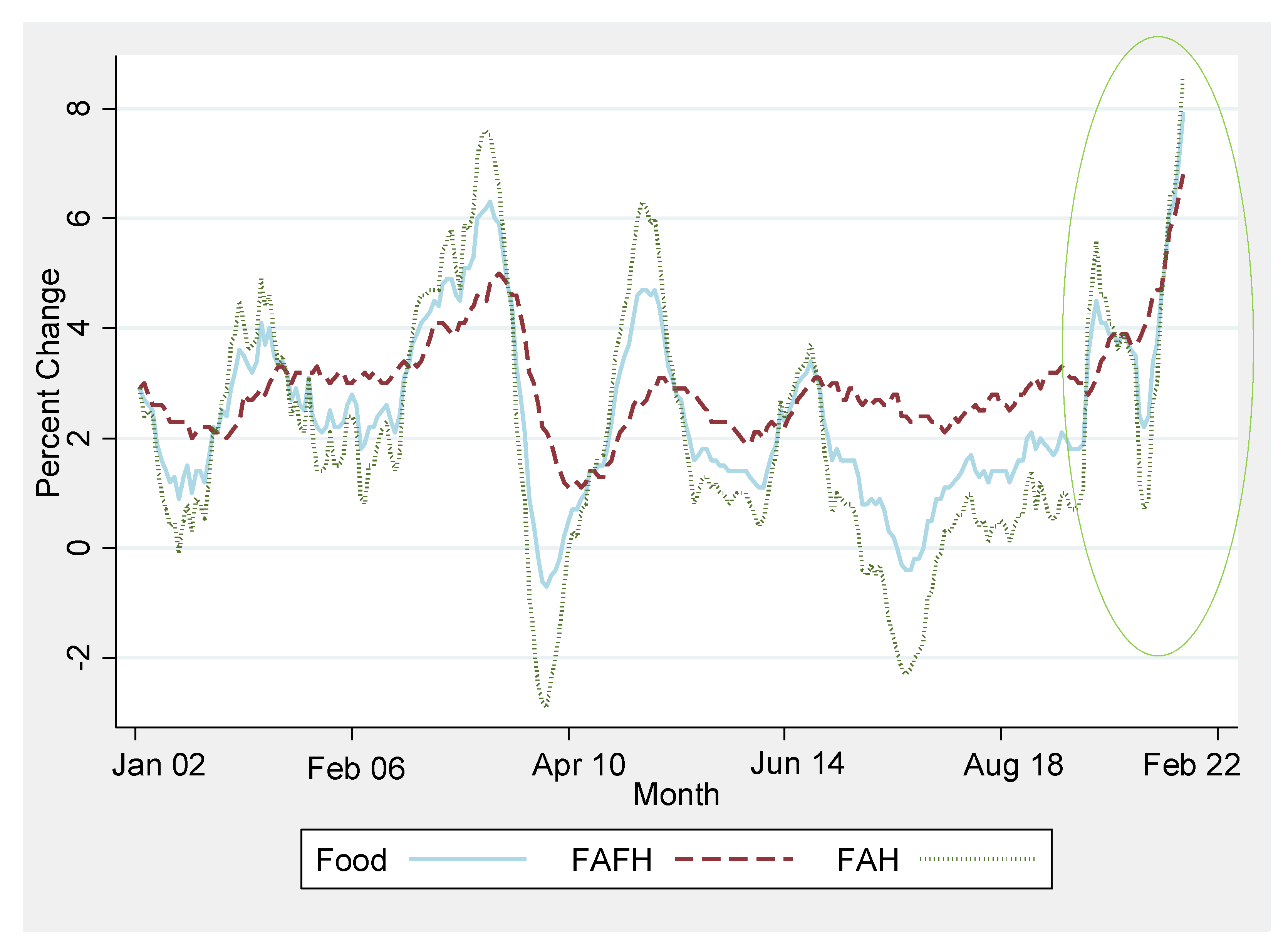
Food prices increased by 7.9% during the month of February 2022 in the U.S. [
1]. This corresponds to the largest annual food price increase in 40 years. The price surge primarily originated from a disruption in the food supply chains due to the COVID-19 pandemic [
2]. This unique food price shock placed a great financial pressure on the budgets of consumers [
3]. This price crisis entails both food at home (FAH) and FAFH. At the household level, exposure to the price shock varied across different regions of the country. The highest increase occurred in the Southern region, while the lowest increase happened in the Northeast.
For instance, at the starting point of the crisis, in the year 2020, the all-item consumer price index encountered an annual increase of 1.1% in the Northeast region of the U.S., whereas the Southern region faced a higher increase of 1.6%. Similarly, the Western and Midwest regions of the U.S. faced an increase of 1.4% and 1.2.%, respectively. The resulting difference in percent increase between the Northeast and Southern regions equals one-half of a percent.
Figure 1 illustrates the twelve-month percentage changes in price indexes for the last twenty years, starting from January 2002. The price shock under consideration in this research is highlighted with the ovoid shape on the right side of the graph.
This study aimed to shed light on the factors that determined U.S. household expenditure patterns for food products in the context of the price surge. For this purpose, the research question is to evaluate how likely households, faced with a price shock, purchase food products and to investigate the intensity of household food expenditures. For this study, all food includes FAH and FAFH. In our paper, the main idea developed rests on the influence of a price surge on expenditure patterns for FAH, FAFH, and all food. However, because all food and FAH exhibit the same shape of price variations, we focus the analysis on all food and FAFH. Chenarides et al. [
4] conducted an online consumer survey in May 2020 in two major metropolitan areas in the United States to investigate food shopping behaviors and consumption during the pandemic lockdown caused by COVID-19. Their findings stressed that food consumption patterns for major FAH groups seemed to stay the same for the majority of the surveyed participants.
Our research contributes to the literature on food demand analysis, in general, by producing new evidence relative to the effects of a particular price shock on food expenditure patterns within U.S. households. To the best of our knowledge, no previous study has addressed this issue, i.e., examining food expenditure patterns for U.S. consumers during a price crisis due to the COVID-19 pandemic. The three findings of this research are the following: First, more than all the other variables, price affected the likelihood to purchase FAH and the propensity to buy FAFH.
Second, price determined the likelihood to purchase FAH, but not significantly the amount spent on the food products in the specific situation of price hikes. In contrast, price significantly determined not only the likelihood to purchase but also the amount spent on FAFH in this unique price crisis experienced by households. Third, consistent with the inelastic nature of food products, conditional expenditure elasticities of income were less than one for food in general and for FAFH.
Based on the results, holding everything else constant, a 10% increase in income is associated with a 1.4% increase in the probability to purchase FAH and a 9.6% increase in propensity to spend on FAFH. However, with respect to price, both FAH and FAFH represent elastic goods during the price shock period. In addition, a 1% increase in own price implies a 7.78% decrease in the probability to spend on FAH (including all kinds of food) and a 20.93% decrease in the propensity to purchase FAFH. The results of this analysis elicit the profile of food products consumers in terms of their socio-demographic traits and location, key economics characteristics same as the inherent seasonal heterogeneity. Doing so, our article provides business managers and marketing experts with options for designing a strategic food-pricing policy. Additionally, food policy-makers can find rigorous indicators relative to the various kinds of disparities in food access that households might be experiencing because of the market price upsurge. Our findings might be useful for them in addressing disparities issues. The remaining sections of this study cover the relevant literature, the data used, the econometric model, the results, and the conclusions.
2. Related Literature
The total spending on food and beverages in the United States was USD 1.8 trillion in 2019 while the annual share of FAFH expenditures reached 51.6 percent, up from 47.3 percent in 1997 [
5]. Saksena et al. [
6] pointed out that FAFH has become increasingly integrated into the American diet. They argued relative price changes represented an important determinant of food choices. Hirvonen et al. [
7] argued that all households increased their consumption of staples relative to other types of foods and concluded that this pattern is much more suggestive of changes in relative prices than in the heterogeneity of demand changes related to income changes. Bozoglu et al. [
8] used a multivariate sample selection model to explore the effects of socio-demographic and economic factors of expenditures on FAFH and FAH in Turkey. Their empirical results highlighted that urban households tend to spend more on FAFH than FAH as incomes have increased.
Household size may also impact FAFH expenditures [
9]. Amoakon et al. [
10] explored the food expenditure patterns of college students in the United States relying on the Engel relation between food expenditures and income. Their findings suggested that the average college student spent about 30% of their income on food while the estimated marginal share was 0.076. Liu et al. [
11], using a Box–Cox double-hurdle model, investigated the effects of household composition along with income and education on FAFH expenditures in urban China. They found that household composition indeed had significant effects on FAFH consumption, both at the participation and expenditure steps. Further, employment and education status were common causes of both FAH and FAFH expenditures. Yet, marital status, race, and sex had mixed effects [
12]. Ogunmodede and Omonona [
13] investigated food consumption patterns and related illnesses among households and found that household consumption patterns were influenced by household-head sex, income, location, level of awareness of plant-based whole food, and total food expenditures. After examining food price shocks and the changing patterns of consumption expenditure across decile classes in rural and urban India, Sinha and Laha [
14] concluded that consumption expenditure differed in both spatial and temporal dimensions.
The COVID-19 pandemic directly impacted both FAH and FAFH expenditures [
15]. Government policies, at the state or city level, mandated the closure of restaurants and other FAFH venues, while local authorities treated grocery stores as essential businesses, in contrast. Expenditures on FAFH significantly declined as a result [
15,
16]. This analysis did not neglect FAFH expenses, rather this subject is a matter of our focus in addition to all food which includes FAH. As a substitution for the decline in FAFH expenditure, some authors [
15,
16,
17] noticed a significant increase in the proportion of households who used online grocery shopping during the pandemic. Similarly, the online SNAP pilot expanded during the pandemic [
16]. Chang and Meyerhoefer [
17] investigated how the coronavirus pandemic affected the demand for online food shopping services in Taiwan and found that some of the increased demand for food products was due to a substitution for FAFH.
Our article aims to extend on how several socio-demographic factors, among others, affect food expenditure patterns when U.S. households were impacted by a price shock. Because race and ethnicity are complex concepts and based on constructs, they need to be explained within a rigorous framework, and their relevance for this paper is pointed out. As socio-demographic factors, race and ethnicity are concepts of major importance in the U.S. They are sources of diversities. Alesina and La Ferrara [
18] argued that an ethnic mix brings about variety in experiences and cultures which may be productive and may lead to innovation and creativity. For them, racially mixed cities are constant producers of innovation in business. In the U.S., race and ethnicity are also sources of disparities [
19]. For example, the racial disparities span both income and access to food. Because race-related differences in economic outcomes have been a long-lasting concern in America, we found it pertinent to include the issues of race and ethnicity factors in our model. In accordance with almost all the previous studies on food expenditures patterns, we assume that, in conjunction with the other factors, race and ethnicity play a crucial role as determinants of household food expenditures. For this paper, ethnicity identifies whether or not the head of the household is Hispanic. Thus, race defines all the non-Hispanic racial groups, for instance, Black, White, Asian, American Indian, and Pacific Islander, same as the other minorities. Before the COVID-19 pandemic, from the year 2017 to 2018, more than one-third of U.S. adults consumed fast food on a typical day, with the highest levels among non-Hispanic Black people [
20]. The coronavirus pandemic has disproportionately impacted the racial and ethnic communities across the territory of the U.S. [
21]. Ellison et al. [
16] stressed that, in America, the pandemic could exacerbate inequalities and disparities in food access. It is relevant for this article to not only answer how race and ethnicity determined the food spending behavior of U.S. households in the context of COVID-19 but also to shed light on the inherent disparities.
Deaton and Muellbauer [
22] explained the influence of the economics factors on food consumption and found incomes and prices most importantly determined the consumer behavior for quantity and types of food bought. According to Engel’s law, the less wealthy a household is, the greater the proportion of total food expenditure. By contrast, the wealthier a household, the smaller the share of expenditure on food for total expenditure. Additionally, consumption of foods such as fresh fruits or meats increased with rising income, while consumption of basic foods such as potatoes and cereals, considered inferior goods, decreased with increasing income. However, consistent with Engel’s law, most food products are inelastic goods. Understanding the transformation that occurs in food expenditure patterns in response to a rapid price increase is a topic of interest for marketers, researchers, and policy makers. Reiss and White [
23] showed that U.S. households strikingly changed their energy consumption habits in response to a price shock confined to California state. Bitler et al. [
3] focused on the EBT payment effect on food hardship rather than spending behavior changes. Bauer et al. [
24] investigated the impact of governmental assistances on low-income households. Garner et al. [
25] elaborated on the descriptive analysis of the reported changes in behavior and concluded that the price crisis profoundly affected consumer spending patterns and suggested a more detailed multivariate investigation.
This paper lines up more with the research works on measuring the economic consequences of the ongoing market price crisis. Establishing not only on the theory of price and income relative to food consumption patterns but also considering how households can change their consumption expenditures on food products in the context of a price crisis, we formulated the testable hypothesis that the price shock affected not only the likelihood to purchase food products but also the expenditure level devoted to food products.
3. Materials and Methods
3.1. Data Description
To estimate the factors that determine the U.S. household expenditure patterns for food products in the context of price shocks, this study employed the data of Consumer Expenditure Diary Survey (CEX) for the year 2020. This corresponds to the most recent CEX data available when this paper was undergoing its writing process. Collected quarterly by the Bureau of Labor Statistics (BLS), the CEX data are fully accessible from their website and represent all the U.S. civilian non-institutionalized population. The unit of observation corresponds to the surveyed household. To be specific, the CEX gathers a wide range of data related to the purchases made by the households, including large spending, such as vehicles and property, same as regular spending, such as food expenditures and rents. Furthermore, the CEX provides detailed socio-demographic information such as family size, employment status, race, gender, marital status, age, annual wage, and welfare program involvement and received benefit amounts.
During each quarter, the Census Field Representative places the Diary Survey booklet in the household to be surveyed for two consecutive weeks. During these time windows, the respondents record expenditures for 7 consecutive days, i.e., the diary week. Each Diary Survey week is assigned to the Diary Survey quarter in which it was recorded. Thus, all Diary Survey files are organized as quarterly data. This research exploits the diary data spanning all four quarters of the year 2020. After cleaning the sample, mainly from 15 cases of households exhibiting negative income before tax, our full sample size equaled 10,453 observations. After examining the dataset, we found that each household was interviewed only once. Therefore, the full sample contains as many households as observations.
Consequently, to estimate the expenditure patterns of U.S. households while they faced an exceptional price shock for food products, our analysis relied on a set of four types of variables widely used in the analysis of food consumption patterns, namely the socio-demographic characteristics of the households, their geographical location, the seasonal trend, and price variables. Capps [
26] employed these four kinds of variables to analyze the U.S. consumer expenditure patterns for fish and shellfish. Identical to Byrne et al. [
27], except the price variable, who examined the expenditure patterns of U.S. households for FAFH from 1982 to 1989. Zhao et al. [
28] retained the same variables to evaluate the U.S. consumer expenditure patterns for fresh flowers. Recently, Cheng et al. [
29] included the four types of variables to estimate demand for nuts in the U.S. Dettmann and Dimitri [
30] had only focused on the socio-demographic characteristics to examine the expenditure patterns of U.S. consumers of organic vegetables.
Incorporation in our analysis of regional dummy variables intends to measure the differences in location-specific effects regarding expenditures on food products and FAFH at the household level. Seasonal dummy variables aim to capture the differences in expenditures by season (either warm or cold). Furthermore, variables such as income before tax, household size, age, education level, sex, marital status, race, housing status, and Supplemental Nutrition Assistance Program (SNAP) participation are introduced to control for the effects induced by the socio-demographic characteristics on the spending patterns of households. Following Capps [
26], we used Consumer Price Index (CPI) as the price variable. We obtained the CPI data from the BLS website, the institution that collects them.
Table 1 reports the summary statistics for both the dependent and independent variables used in this research in addition to their definition.
Because CPI is available monthly, we constructed a quarterly CPI for this study for FAH including all food and FAFH by averaging the monthly CPI over each quarter. From these quarterly CPI, we generated the corresponding price variable for every single observation in our dataset. Using CPI as price variable is relevant for this study in the sense that it captures the average changes over time in prices of fixed basket of goods and services of constant quality and quantity for urban consumers. Moreover, CPI reflects the spending pattern for all urban consumers and wage earners, spanning 93 percent of the total U.S. population.
3.2. The Model
3.2.1. Identification Strategy
Related to econometric issues such as censored responses, truncated data, or sample selection bias, zero expenditure is a concern characterized in empirical estimation of food expenditure patterns, as intended in this study. Also known as limited dependent variable issue, ignoring zero expenditure and estimating the expenditure function by a single equation using ordinary least square (OLS) regression method results in potential bias and inconsistency of the parameter estimates. To be precise, two issues can arise: sample selection bias and censored observations, concerns encountered in this paper with the CEX Diary data we employed. For instance, in the final sample, censored observations represent 9.05% for all-food subsample, 36.55% for FAFH subsample, and 16.70% concerning FAH subsample. Fortunately, the econometric literature provides several methods to handle these two concerns inherent with the estimation of food demand.
Among these models, three are widely used by economists: One is the Tobit model [
31]. It is a single-equation model. The Tobit technique restricts the directional effects to be identical for the decision to consume along with the intensity of expenditure share. Additionally, this model treats the choice to consume and the consumption-level decision as joint, thus providing a unique parameter estimate for both. Regardless of its weakness, Tobit is a well-known method and appropriate to handle censored response issues. However, we do not estimate the Tobit model in this paper for the need to distinguish between the decision to consume and the level of consumption.
The double-hurdle model [
32,
33] is another model to handle zero expenditure problem. Unlike the Tobit model, this method uses a double-equation model, which offers the ability to estimate the parameter estimates separately for the decision to consume and the consumption level decision. An alternative to the double-hurdle method is the Heckman two-step model [
34]. Suitable to data with sample selection issue, the Heckman two-step technique is a double-equation model, which distinctly estimates the decision to consume and the choice level. More importantly, this model corrects for sample selection bias and provides consistent parameter estimates.
It urges to clarify the distinction between the double-hurdle and the Heckman two-step models. From the standpoint of the first model, zero expenditure is due to consumers who choose not to participate in the decision-making stage, same as those not spending during the consumption stage due to some factors [
32]. Oppositely, the second model considers zero expenditure to occur predominantly during the selection stage, while positive expenditure is involved at the consumption step [
34]. Otherwise stated, the Heckman two-step model, unlike the double-hurdle model, assumes the quasi absence of zero expenditure in the second stage once the first stage or selection step is passed. But the double-hurdle considers the possibility of zero outcome in the participation stage. This article relies on Heckman approach and believes that zero expenditure occurs only predominantly during the selection stage. In addition, when inaccurate data source or self-retention justify the presence of zero expenditure, the double-hurdle model is more recommended [
35]. But when zero consumption results from purchase infrequency, especially when the reference period is short as weekly, the Box–Cox hurdle model is applied [
36,
37]. Because this paper used quarterly data, we assume that purchase infrequency is not a major concern; also, our CEX Diary data are exempt of any serious inaccuracy concerns. Therefore, we will only estimate the Heckman two-step model to investigate the expenditure patterns for food products under the context of price crisis.
Byrne et al. [
27] and Zhao et al. [
28], the same as Dettmann and Dimitri [
30], used Heckman two-step as their empirical model to estimate expenditure patterns. Cheng et al. [
29] used it to estimate consumption of nuts in the U.S. Following Cheng et al. [
29], but unlike the previous studies [
27,
28,
30], we added the price variable to the empirical model. We assumed that the effect of price on the expenditure patterns could be evaluated separately from other region-specific effects. The consumers can be expected to become more price sensitive in the context of COVID-19 crisis [
15].
Early in the data section, we have already showed the arguments supporting the independent variables involved in our regression model. Further, the regressors successfully passed the test for variance inflation factor (VIF). Accordingly, the VIF for each of the explanatory variables was less than 10, and all ratio 1/VIF were non-negative. The VIF test served to establish that our empirical model is free of any multicollinearity issues.
Table 2 presents the details of the VIF test.
3.2.2. Heckman Two-Step Empirical Model
This article aimed to estimate the expenditure patterns of U.S. households while they faced an exceptional price shock for food products. For this purpose, we assumed that spending on food products was a two-step process decision. First, the consumer decides whether to purchase food products. Second, the household decides the level of spending share to be devoted to the chosen food products. In other words, this process refers to a two-stage decision mechanism for the consumer. This mechanism connects the first stage to a participation decision, while the second stage is associated with the expenditure-level decision.
Following Heckman [
34], the purchase decision for food products and the amount spent on purchasing has been modeled through two separate regressions. In accordance with the Heckman two-step approach, the first stage involves a Probit regression allowing to access the probability of participation in food products consumption, while the second stage employs an OLS regression to determine the level of expenditures on the food items. By adopting a traditional Heckman two-step, the second stage estimation omitted all zero observations for the dependent variable, for instance, expenditure on food or FAFH.
Table 3 reports the descriptive statistics for the subsamples of households with non-zero expenditures on all food, FAFH, and FAH. However, a potential sample selection bias may occur with the OLS regression while dropping the zero expenditures. To correct for the sample selection bias, Heckman proposes the inverse Mills ratio, a specification derived from the first stage and included in the second-stage estimation, which serves as instrument for the omitted variables.
Also known as selection equation, the first stage of Heckman two-step is modeled through a Probit method as presented in Equation (1).
where
= 1 represents a household that bought food or FAFH, Pr {…} is for probability, and i = 1, ……, N refers to all the households in the uncensored sample.
corresponds to the vector of all the explanatory variables.
Table 1 exhibits more details for all the explanatory variables included.
denotes the vector of the coefficients to be estimated while
is the error term.
Estimated from the Probit regression, the inverse Mills ratio connects the participation decision and the expenditure-level decision. The ratio is computed as presented in Equation (2).
where
is the inverse Mills ratio calculated for every single consumer unit.
corresponds to the density function, and
refers to the cumulative distribution function of the normal distribution.
It follows that the second stage or outcome equation of Heckman procedure is modeled with an OLS regression as presented in Equation (3).
where
corresponds to the amount spent by the household to purchase food product.
is the inverse Mills ratio and
is its equivalent parameter estimate.
represents the same explanatory variables included in the Probit regression, except the variable housing status dummies that was excluded to account for the exigence to restrict at least one variable between the first and second stage of Heckman two-step estimation method.
is a vector of the estimated expenditure coefficients. Finally,
is the error term regarding the outcome equation. We estimate the above-exposed Heckman model through the two-step command of STATA that allows us to estimate simultaneously both the Probit and the OLS regression.
Equation (4) reports the conditional marginal effects formula, while Equation (5) presents the conditional elasticity formula.
where
refers to the conditional expectation function from the second stage, Equation (3).
is the partial derivative of the inverse Mills ratio with respect to
, any explanatory variable used in both stages of the model.
4. Results
In this paper, using the Heckman two-step model, we estimate the expenditure patterns of U.S. households while they experience a unique price shock for all food products. The following sections expose the results obtained through the Probit and the OLS regressions.
4.1. Households’ Likelihood to Spend on Food Products
When challenged by a price shock, the households firstly decide whether to purchase food products. Accounting for a situation of a price surge, we estimate the factors that determine the propensity of the U.S. consumer units to simply buy or not buy any food products but also to spend or not spend on FAFH. The first stage of the Heckman model serves to elucidate the direction of the likelihood to spend on food, all kind included, or just FAFH. Yet, except for the direction, the magnitudes obtained from the participation stage are meaningless. For this reason, we computed the conditional marginal effects to capture more precision about the parameters.
4.1.1. Likelihood to Purchase Food including Food at Home
The findings from the participation stage, column 1 of
Table 4, highlight that price has a significantly negative effect associated with the likelihood to purchase food. The conditional marginal effect on price indicates that the households have a decreasing tendency to purchase food, all kind included, when prices rise. Income before tax exhibits a significant positive relationship with the propensity to buy food. For the sampled consumer units, the conditional marginal effect stresses that an increase in income is associated with a higher propensity to buy food. This is consistent with Byrne et al. [
19] who found a positive relationship between income and the likelihood to purchase food. But participating in SNAP had a significantly negative link with the likelihood to purchase food. The estimated results suggest that the households which earn a low income and benefit from SNAP are less likely to buy food compared to those that are not SNAP participants. A statistically significant regional difference occurs in the likelihood to consume food. Compared to the households living in the Midwest region, those residing in the Southern region of the U.S. were less likely to acquire food through the market. However, the findings from our sample suggested that living either in the Northeast or in the Western region had no significant link with the propensity to purchase food.
Our results pointed out that marital status, education level, seasonal trend, race, and ethnicity showed a significant effect on the probability to purchase food. It follows that the married had more tendency than the unmarried to purchase food. Compared to the household headed by someone who attended high school but without graduating, those headed by highly educated people, a bachelor’s, master’s, or Ph.D. holder, were more likely to buy food. Spending on food more likely occurred during the first and fourth quarters, i.e., the cold season, than during the warm season. A household headed by a Black individual was less likely to purchase food. Compared to non-Hispanic people, a household led by a Hispanic person was significantly more likely to purchase food. However, the variables such as household size, age of the reference person in the household, sex of the reference person, number of dependents younger than 18 years old, and housing status, each of them separately taken, had a statistically insignificant effect on the likelihood to purchase food according to the sample analyzed. Relatively, these findings emphasized that price affected the likelihood to purchase food more than all the other variables.
4.1.2. Likelihood to Buy Food Away from Home
From the participation stage, column 3 of
Table 4, the sample results stress that price had a significantly negative relationship with the likelihood to buy FAFH. The conditional marginal effect on price signals that the households had a decreasing propensity to purchase FAFH when prices surged. Income before tax exhibited a significant positive relationship with the likelihood to buy FAFH. The conditional marginal effect stressed that an increase in income is associated with a higher propensity to buy FAFH. But participating in SNAP had a significantly negative association with the likelihood to purchase FAFH. The households which earned a low income and benefited from SNAP were less likely to buy FAFH relative to those who did not use SNAP. The findings demonstrated a statistically significant regional difference in the likelihood to consume FAFH. The households, whether they were in the Northeast or in the South, were less likely to purchase FAFH relative to those in the Midwest region. Results from our sample suggested that living in the Western region had no significant relationship with the likelihood to purchase FAFH.
Our findings suggested age, marital status, education level, seasonal trend, race, sex of the reference person, and housing status showed a significant effect on the probability to consume FAFH. Households headed by a person between 40 and 65 years old were more likely to purchase FAFH relative to those headed by a person younger than 40 years old. The consumer units led by a married person had more tendency than those led by an unmarried individual to purchase FAFH. The consumer units headed by highly educated people, i.e., bachelor’s, master’s, or Ph.D. holders, were more likely to buy FAFH compared to those headed by someone who attended high school with no degree. Spending on FAFH more likely occurred during the cold season than during the warm season, i.e., the second and third quarters. When the household was headed either by a Black person or an Asian person, the consumer unit was less likely to purchase FAFH. The households led by a male were more likely to consume FAFH than those led by a female. Also, a reference person residing in student housing was more likely to buy FAFH. Yet, the variables such as household size, ethnicity, and number of dependents having an age less than 18 years old, each of them separately taken, did not have a statistically significant effect on the likelihood to purchase food according to the sample analyzed. Results highlighted that, relatively, price affected the likelihood to purchase FAFH more than all the other variables in the model.
4.2. Intensity of Household Expenditures on Food Products
When challenged by a price surge, after deciding whether to purchase food products in a first step, the households decided in a second step how much to spend on the chosen food products. Under a situation of high price shock, we estimated the factors that determined the amount that the U.S. households spent on any chosen food product. The second stage of the Heckman model served to measure the intensity of the expenditure share on food, all kind included, and FAFH.
4.2.1. Intensity of Expenditures on All Food
From the expenditure stage, column 2 of
Table 4, our estimated results suggested that price had no significant effect on the expenditure shares on food products in general. For instance, price determined the likelihood to purchase food but insignificantly affected the amount spent on food product in this special situation of a price crisis. Our sample results pointed out that as income or size increased, holding everything else constant, the households consistently spent more on food products. Findings also suggested a regional difference in expenditures for food by the households. Compared to the households in the Midwest, the households in the Northeast and West consistently spent less on food in general. Relative to the warm season, i.e., the second and third quarters, the cold season was associated with significantly more expenditures on food. Consistently, expenditures on food products for households headed by highly educated people were higher than food expenditures for a household led by a person who attended only high school with no degree. Married couples significantly spent more on food than unmarried people. The findings suggested a racial difference because Black people consistently spent less on food than White people. The remaining variables did not have a significant effect on the intensity of the amount a consumer unit spends on food for this unique situation of a market price crisis.
4.2.2. Food Away from Home Expenditure
As shown in
Table 4, our estimated results established that price had a significant effect on the expenditure devoted to FAFH. Price significantly determines not only the likelihood to purchase FAFH but also the amount spent on the FAFH under this circumstance of a price crisis experienced by the households included in the sample analyzed. A price increase, holding everything else constant, implied a significant decrease in household expenditures on FAFH. Our finding contrasts with results from Capps [
26], using a quadratic expenditure model, that increases in price, i.e., CPI as in this paper, led to concomitant increases in household expenditures on fish and shellfish. But fish products and FAFH may exhibit some distinct qualities related to unobserved heterogeneity that the consumers interpret differently.
Our findings indicated that as incomes increased, holding everything else constant, the households consistently spent more on FAFH. Compared to the households that were not SNAP beneficiaries, the participant households consistently spent less on FAFH. Obviously, a SNAP voucher does not allow for buying FAFH. Once the household had decided to consume FAFH, our results suggest an absence in regional difference in the amount spent on FAFH. Compared to the warm season, the cold season, for instance, the first and fourth quarters, is associated with significantly more expenditure on FAFH. Expenditures on FAFH for a household headed by a highly educated person were consistently higher than FAFH expenditures by a household led by a person with lower education or no degree. Married people significantly spent more on FAFH than unmarried people. Households with a person whose age is more than 40 years old consistently spent less on FAFH compared to a household headed by a person younger than 40 years old. The findings suggest a racial difference because Black people and Asian people consistently spent less on FAFH than White people, but Asian people spent relatively less on FAFH compared to Black people. The remaining variables did not have a significant effect on the intensity of the amount a household devotes to FAFH in general.
4.3. Conditional Expenditure Elasticities
Table 5 presents the conditional expenditure elasticity of price, income, and size on the probability to consume food in general (which includes FAH) or FAFH. Consistent with the inelastic nature of food products, conditional expenditure elasticities of income were less than one for food in general and FAFH, specifically. Holding everything else constant, a 10% increase in income was associated with a 1.4% increase in the probability to purchase food (including FAH) and a 9.6% increase in the propensity to spend on FAFH. But relative to price, both food and FAFH represent elastic goods in this unique situation of a price shock. A 1% increase in own price implies a 7.78% decrease in the probability to spend on all food and a 20.93% decrease in the propensity to purchase FAFH. This is consistent with Saksena et al. [
6] who showed that the price effect generally caused the quantity of FAFH demanded to decline, depending on the degree of price elasticity. While the conditional elasticities of price and income were all statistically significant at the 1% level, our sample results demonstrated that the conditional elasticities of household size and number of dependents younger than 18 years old were statistically insignificant.
5. Discussion, Conclusions, and Policy Implications
The goal of this study was to understand the factors that determined U.S. household expenditure patterns for food products in the context of the exceptional price shocks due to the COVID-19 pandemic. For this purpose, our analysis relied on the Consumer Expenditure Diary Survey (CEX) for the year 2020. In this study, the household or consumer unit represented the unit of observation, and total food expenditures, spending on FAFH, in addition to FAH expenses were investigated. With a sample size of 10,453 observations, the empirical estimation of the Heckman two-step model provided the following interesting results:
First, the Wald Chi-squared tests were statistically significant at the 1% level for each of the three food products. This suggests the existence of the sample selection bias. Because sample selection bias was present, the adoption of the Heckman selection model was justified. Second, except FAH, the estimated Mills ratio coefficient was statistically significant at the 1% level for FAFH and at the 10% level for all food including FAH. For these two late cases, our results establish that the selection bias was appropriately corrected. Such an argument also justifies why our analysis less involves the estimated results which are relative to FAH. Nonetheless, our model produced consistent and asymptotically efficient estimates for all the parameters regarding all food and FAFH. We could not estimate the expenditure levels and obtain the results without first accounting for the decision to purchase food products. Consistent with Chenarides et al. [
4], taken separately, major FAH groups were less influenced by the price crisis.
Third, consistent with Byrne et al. [
27], we found a positive relationship between income and the likelihood to purchase all food (including FAH). But participating in SNAP had a significant negative link with the likelihood to purchase food. Fourth, relatively more than all the other variables, price affected the likelihood to buy food but also the propensity to consume FAFH. Fifth, price determined the likelihood to acquire food, but for the amount spent on the food products in the particular situation of a price crisis, the estimation was statistically insignificant. Oppositely, for FAFH, price significantly determined the probability to purchase, the same as the amount devoted to purchase in this unique situation of a price crisis experienced by households in our sample. Sixth, consistent with the inelastic nature of food products, conditional expenditure elasticities of income were less than one for both food, in general, and FAFH, specifically. Holding everything else constant, a 10% increase in income was associated with a 1.4% increase in the probability to purchase food and a 9.6% increase in the propensity to spend on FAFH. Seventh, relative to price, both food and FAFH were exemplified to be elastic goods in this special situation of a price shock. A 1% increase in own price implied a 7.78% decrease in the probability to spend on food including FAH and a 20.93% decrease in the propensity to purchase FAFH. Price effects generally caused the quantity of FAFH demand to decline [
6] more drastically than the demand quantity of all food.
Given that our results shed light on the characteristics of food products consumers in terms of their socio-demographic traits and location, key economics characteristics same as the inherent seasonal heterogeneity in a situation of a price crisis, business managers and marketing experts may find some key elements to elaborate their pricing strategy. Food policy-makers can find rigorous indicators to identify and assist the households that might be experiencing disparities in food access because of the market price upsurge. One limitation of this article ties with the impossibilities to produce evidence on the substitution and complementarity links between FAFH and FAH. The econometric model that we estimated does not permit it. Future research may extend on this avenue by estimating an appropriate complete demand model to exemplify such missing evidence from the present article. Future research may also consider online food shopping to further investigate this problem of U.S. household food demand in a context of an exceptional price shock.


