1. Introduction
The spread of the COVID-19 health crisis has created turmoil and a climate of uncertainty in financial markets and businesses, among other effects, and this is reflected in the case of the United States [
1,
2]. Measures to curb the spread of the COVID-19 pandemic in the community and changes in consumer behavior have affected the economies of states, including the economy of the US [
3,
4,
5]. In the international literature, a comprehensive determination of the effects of the COVID-19 pandemic on the US economy has not been recorded, and this is normal as the pandemic is ongoing and continues to create new effects. What have been captured in the international literature are the economic impact assessments and the individual approaches to sectors of the US economy, particularly during the first period of the COVID-19 pandemic [
1,
6,
7]. The research of Walmsley et al. [
3], which estimated the impact on the economy and on employment of a quarterly lockdown in the US, showed that GDP fell by 20.3 percent year on year to USD 4.3 trillion. The financial cost of the first two months spent fighting the pandemic in the US was estimated by Makridis and Hartley [
8] at USD 2.14 trillion. The stock returns of 125 sectors in the US during the COVID-19 period, examined by Thorbecke’s research [
4], showed that the recovery of large parts of the economy does not depend on the microeconomic environment but on the control of the health crisis itself.
The effects of the COVID-19 pandemic on US small- and medium-sized enterprises had a negative impact on their sales. Bloom et al. [
1] surveyed a sample of 2050 small- and medium-sized enterprises, which in the 2nd quarter of 2020 reached an average sales loss of 29 percent. Changes in oil demand during the COVID-19 period in the US affected the economy and the stability of the global energy chain [
9,
10]. The fear and uncertainty created by the COVID-19 pandemic affected all stock markets, including in the United States [
2], especially during the first period of the pandemic [
11]. The strengthening of the instability of the financial markets in the US is also confirmed by the research of Albulescu [
12]. Qureshi’s [
13] research assessing the impact of the COVID-19 pandemic in the US on economic indicators showed that the pandemic had a strong impact on long-term forecast economic variables. On the other hand, the cost–benefit analysis of the first wave of COVID-19 in the US, from the state repression policies investigated by Broughel and Kotrous [
14], showed that the total economic benefits in production from the beginning of April to 1 August 2020 ranged between USD 632.5 billion and USD 765 billion, while the cost of the repression policies ranged between USD 214.2 billion and USD 331.5 billion. Other research agrees that the scales are tilted to the benefit side [
15,
16]. Goolsbee and Syverson’s research [
17] attributed the recession not to the lockdown policies imposed but to the very behavior of the consumer public that reduced consumption under the fear of contamination. In addition, it has to be taken into consideration that the medical cost is high [
18], and it has a major impact on the US economy [
19].
Drawing upon the fact that the US economy is suffering from a reduction in production and employment losses higher and more severe than the latest financial crisis, this paper aims to expand our current knowledge on the effects of the COVID-19 economy by investigating key sectors and the structural capabilities of the US economy. It therefore highlights the drivers of economic growth by considering the output, employment, and import multipliers and identifying the key sectors, not only for a short-term effective demand management policy, but also for a long-term structural policy.
More specifically, an essential question for any economy concerns which sectors the policy makers should spend more on for a recovery and resilient plan after a negative shock. There are many different and ambiguous approaches to answering this question, where the spending multipliers are the key factors. Most of these approaches are based on econometric methods, while others apply an IO (input–output) methodology. The main drawbacks of the econometric approaches are characterized by (i) the inability to take into account the interrelationships between the sectors; (ii) the strong sensitivity to the structural breaks; (iii) the availability and the quality of the most recent data; (iv) the need for a “comparison between normal times and bad ones”; and (iv) the difficulty in giving robust valuations in industry/sectoral terms. Conversely, the IO tables can be considered the core of the National Account Systems, as they capture the interrelationships between the sectors, the commodities they produce, and the sectors that use these commodities. Additionally, IO tables have also the advantage that they do not depend on the structural breaks in the data because the structural change of the economy is a long-term process, and therefore, the research can be based on the more recently available IO data. Hence, multipliers that have been estimated on the basis of the structure of IO systems have the advantage of considering the technology of all sectors of the productive system and the technical relations established amongst them, summarizing this complex network of technical relations into single indicators. For this reason, the IO approach is considered more adequate as a basis for a resilient recovery plan.
The purpose of this article is to estimate the output, employment, and import multipliers for the US economy, a few months after the election of the new US president, using the latest data at that time from the OECD IO tables, i.e., the 2015 tables. In contrast with other advanced IO models for measuring the multipliers, our approach is based on an analytical framework that, except for technical conditions of production, also draws attention to the feedback effects of imports, income distribution, savings (out of wages and profits), and consumption patterns. It has to be noted that this framework for studying multiplier effects was constructed by Kurz [
20] and Metcalfe and Steedman [
21]. Further developments in a more generalized framework can be found in Mariolis [
22]. For relative empirical applications, see, e.g., Mariolis and Soklis [
23] and Mariolis et al. [
24]. For extra details on the theoretical framework and more empirical applications, see Demiroglou [
25] and the references therein. Furthermore, it includes, as limit cases, the usual (Keynesian) multiplier [
26] and the multipliers of the traditional input–output analysis [
27]. Thus, this article focuses on intersectoral analysis and especially on indexes for the short-term (i.e., to boost employment and growth) and long-term policies (i.e., to increase productivity and control import dependency). The primary consideration of our results aims to provide insights for policy makers in order to be able to evaluate different plans for the post-COVID-19 era that combine growth and economic efficiency with social cohesion and justice. For those reasons, our empirical evidence is presented in a simple and easy way that allows the policy makers the evaluation of any possible recovery and sustainable program. We chose not to formulate our own alternative plans but to state how our analysis is implemented in an already announced program. We therefore evaluate the impact of the two main pillars of the economic policy of the Joe Biden administration, the American Jobs Plan and the American Families Plan. In general, our findings support the idea that US policy makers have a wide range of sectoral policies to meet the current challenges of the US economy.
The remainder of this paper is structured as follows:
Section 2 of the paper offers an analytical framework, while
Section 3 applies this to the structural economic basis of the US economy.
Section 4 investigates the structure of the elements of the final demand of the US economy and analyzes the growth dynamic of the various sectors based on the multiplier effects of each sector.
Section 5 evaluates the impact of the American Jobs Plan and the American Families Plan. Finally,
Section 6 offers some concluding remarks.
2. Methods and Materials
We assume a linear, open economy of a single production with
sectors and commodities, in which there are two types of income, i.e., income out of wages and income out of profits. The system of the physical quantities of the economy is described by
where
is the vector of the gross outputs of the economy, with dimensions
,
is the square matrix of the direct technical coefficients, each element of which represents the quantity of commodity
necessary to produce one unit of commodity
as the gross output, and
is the vector of the net outputs of the economy, with dimensions
. Solving Equation (1) for
we obtain
The vector of net products of the economy can decomposed as follows
where
is the vector of the final consumption demand of the wage earners, with dimensions
,
is the vector of the final consumption demand of the profit earners, with dimensions
,
is the vector of import demand, with dimensions
, and
is the vector of autonomous demand (gross fixed-capital formation, the government’s final consumption expenditure, and the exports demand), with dimensions
.
The price side of the economic system is given by the following equation
where
is the vector of prices of the commodities of the economy, with dimensions
,
is the diagonal matrix formed by the sectoral profit rates,
is the vector of sectoral wages, with dimensions
,
is the diagonal matrix of the sectoral employment coefficients, and
is the sign of the transpose of a matrix entity. After rearrangement, Equation (3) can be written as
where
and
.
Equations (2) and (5) imply that final consumption demand can be expressed as
and
where
is the propensity to save out of wages,
the propensity to save out of profits, and
is the exogenously given consumption pattern, which, for simplicity’s sake, is assumed to be uniform between the incomes from wages and profits.
Substituting Equations (6) and (7) into Equation (3) we obtain
where
represents the total consumption demand of the economy,
is the total import demand of the economy, and
is the diagonal matrix formed by the elements of
.
Finally, solving Equation (8) for the net outputs of the economy,
, we obtain
where
represents the
matrix, which links the autonomous demand, as represented by the
vector
, with the net product of the economic systems, as represented by the vector
. Thus, the matrix
represents the “multipliers” of the commodities of the economic system, and the values of this matrix depend in a complex way on the socio-technical conditions of the production, the imports, the saving patterns, and the structure of autonomous demand. (For more information on this modelling, see Kurz [
20], Metcalfe and Steedman [
21], Mariolis [
22], Mariolis and Soklis [
23], Mariolis et al. [
24] and Demiroglou [
25])
On the basis of the matrix of mutlipliers, the matrix of employment multipliers is given by
, where
is the matrix of the employment coefficients, i.e., the total employment (direct and indirect) necessary to produce one unit of output for each commodity. Thus, the vector of the levels of employment of each industry,
L, is given by
In a similar way, we may derive the matrix of import multipliers,
, while the vector of imports of each commodity,
, corresponding to different levels of autonomous demand, is given by
In what follows, we apply the previous analysis for the US economy, using data from the IO table for the year 2015, i.e., the latest available data at the time of this research, provided via the OECD’s (Organisation for Economic Co-operation and Development) database,
https://stats.oecd.org (accessed on 5 September 2021), for the polar case where all the wages are consumed and all the profits are saved, i.e., for the case where
and
. In order to apply our analytic framework, we need to extract
,
,
,
,
, and
from the available data. The IO table of the US economy describes the production of 36 commodities by 36 sectors of a single production. Thus, if we denote by
the
matrix of intermediate consumption, directly available from the IO table, then the matrix of direct technical coefficients,
, is derived by
, where
is the
column vector of the sectoral gross outputs, directly available from the IO data, and
is the diagonal matrix formed by the elements of
. Similarly, the elements of the vector of the direct labor coefficients,
, are derived by dividing the total labor employed per sector by the total sectoral gross output. Τhe vector of total import demand,
, is directly available as a relative column in the IO table of the US economy. Similarly, the vector of the consumption pattern is identified with the elements of the column “Final consumption expenditure of households”, directly available from the IO table. The elements of the vector of sectoral wages are derived by dividing the sectoral “Compensation of employees” by the total labor employed in each sector. Finally, the price vector
is identified with the summation vector
, i.e., the physical quantity of measurement of each commodity is set equal to that quantity which is worth one monetary unit. (The monetary unit in the IO table of the US economy is set to be equal to USD 1 million.)
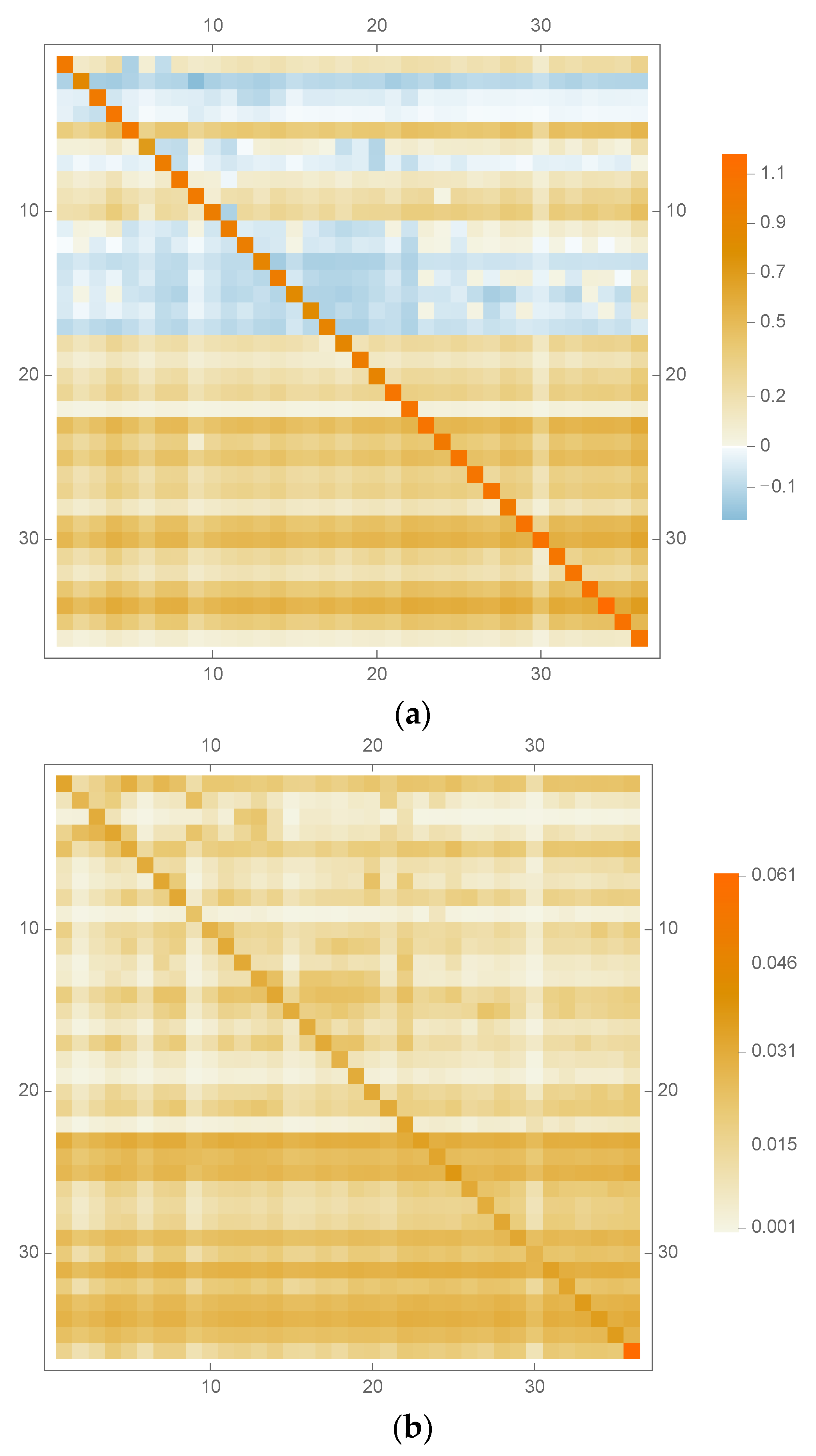
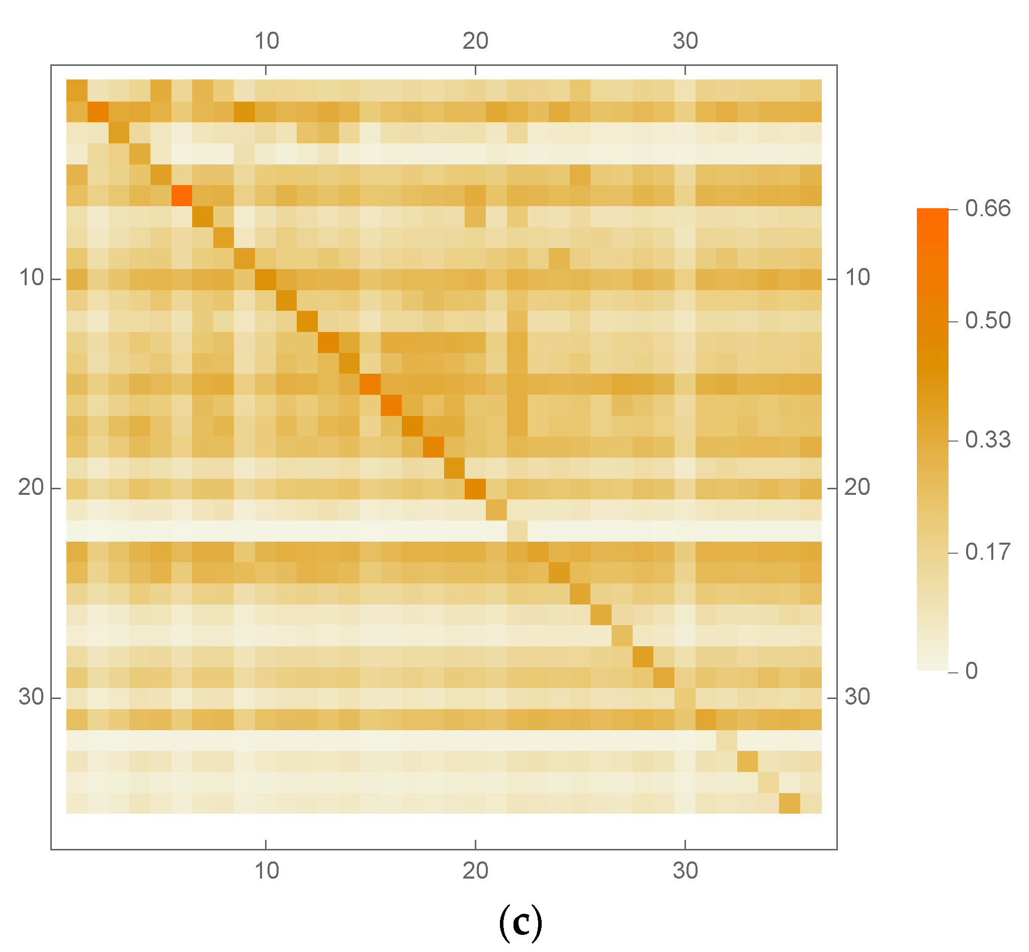
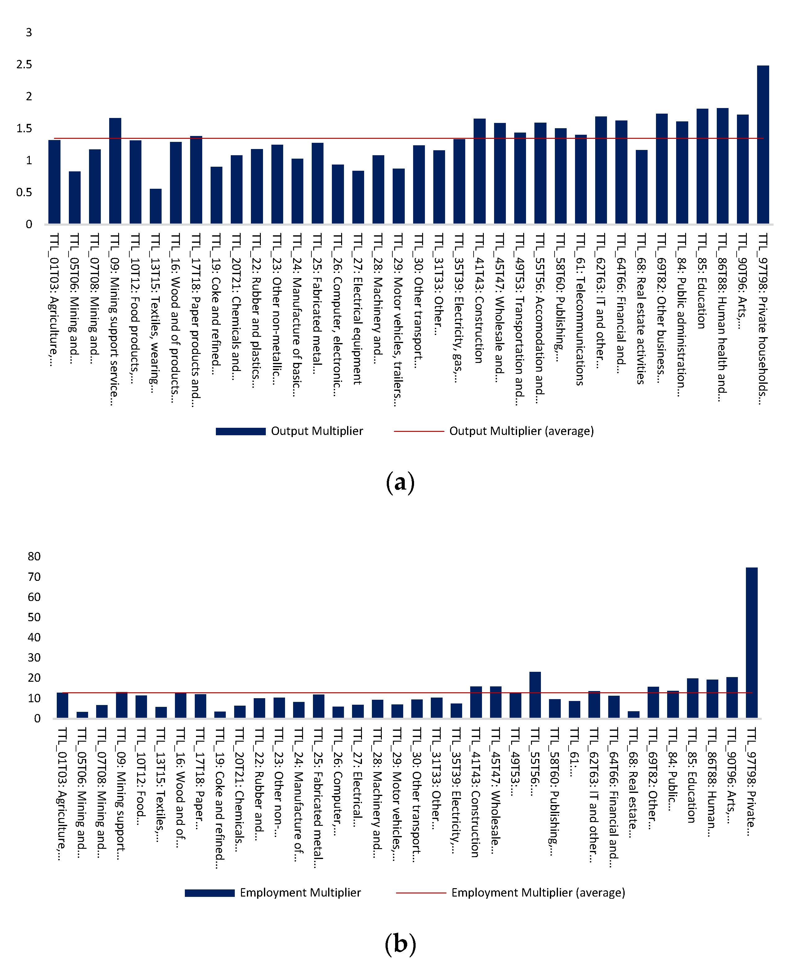
To obtain a general picture of the basic elements of the analysis, in
Figure 1,
Figure 2 and
Figure 3 we provide the matrix plots of the output, employment, and import multipliers (see Equations (9)–(11), respectively) of the US economy. Commodities 1–4 belong to primary production. Commodities 5–22 belong to industry. Commodities 23–36 belong to services.
From the plots of the matrix multipliers, we observe that favorable multiplier effects are concentrated mainly with the services. Now, we can proceed to the following definitions. (For more details, see Mariolis et al. [
24]). We characterize as a key commodity each commodity that simultaneously demonstrates (i) the average output and employment multiplier indices that are above the economy’s average and (ii) the average import multiplier indices that are below the economy’s average. More specifically, these key commodities are considered as appropriate for the implementation of a demand policy in the short term, i.e., for boosting growth and job creation. Moreover, we characterize as key commodities for a long-term, structural policy each commodity that is characterized by (i) an average ratio of output to employment multiplier indices that is above the economy’s average and (ii) an average ratio of output to import multiplier indices that is above the economy’s average. The former ratio can be conceived as a productivity index of each commodity, while the latter can be conceived as an import dependency index of the economy. Hence, a long-term, growth-oriented, structural policy should also consider those two types of multiplier indices.
3. The Structural Economic Basis of the US Economy
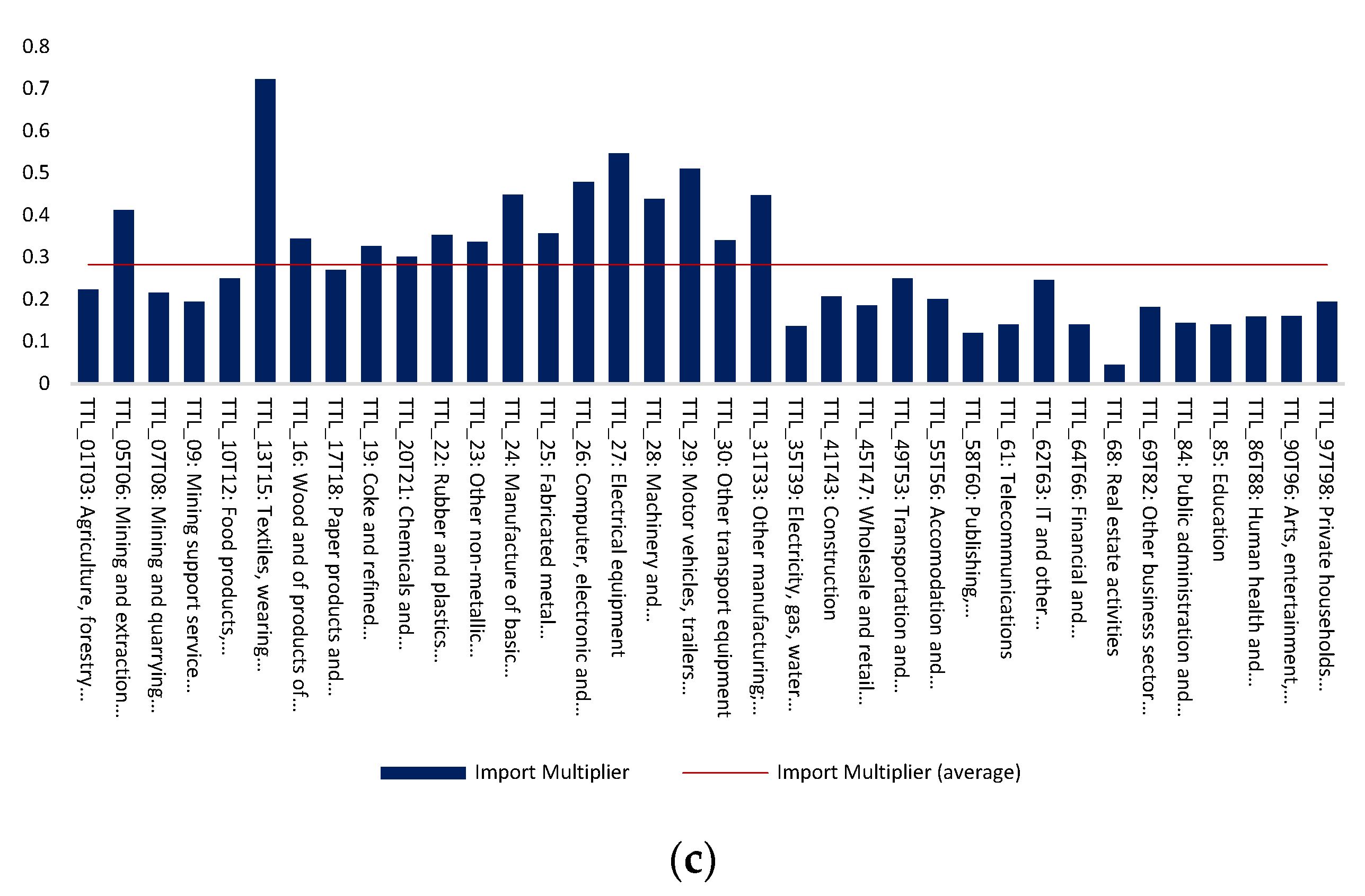
Based on the previous analysis, and using data from the input–output (IO) table of the US economy for the year 2015, we estimate the output, import, and employment multipliers for the 36 different commodities/sectors that are described in the IO table (
Figure 2). The first column of
Figure 2a–c indicates that a change of 1 monetary unit in the demand for “Agriculture, forestry and fishing” induces a change of 1.32 units in product output, a change of 12.76 employment units, and a change of 0.22 units in imports, respectively. The remaining columns of these figures are constructed in a similar way. Hence, a change of USD 1 million in demand causes an average change of USD 1.35 million in product output, a change of 12.87 persons employed in the production, and a change of USD 0.28 million in imports. (All the detailed empirical results are available on request. It is also noted that the construction of the relevant empirical variables necessary for the empirical analysis was based on the usual procedure followed in other similar studies in the field (see, e.g., Mariolis et al. [
28], Appendix A1).)
We observe that the key commodities for effective demand management policy are “Mining support service activities”, “Construction”, “Wholesale and retail trade; repair of motor vehicles”, “Transportation and storage”, “Accommodation and food services”, “IT and other information services”, “Other business sector services”, “Public administration and defense; compulsory social security”, “Education”, “Human health and social work”, “Arts, entertainment, recreation and other service activities”, and “Private households with employed persons”. Hence, leaving aside the construction sector, all the key commodities detected in the US economy correspond to sectors of services. This finding is not unexpected if we consider the structure of the matrix multipliers of the US economy (see also
Figure 1 above). These commodities are characterized by output and employment multipliers that are above the economy’s average and, at the same time, by import multipliers that are below the economy’s average. Thus, the economic policy authorities could implement an effective demand management policy by stimulating demand for these commodities. Such a policy could lead to a significant increase in output and employment without affecting in a negative way the external sector of the economy. To further delve into this finding, in
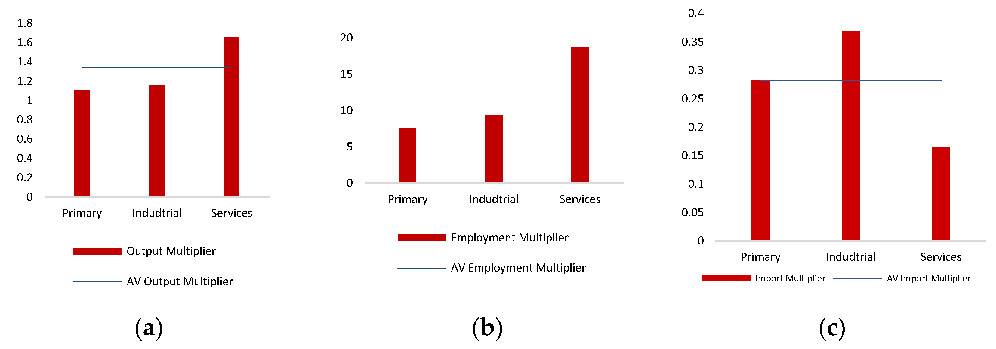
Figure 3 we present the average output, import, and employment multipliers for primary production, industry, and services.
Reading
Figure 3 in the same way as
Figure 2, we confirm that services is the only sector that demonstrates favorable output, import, and employment multipliers. However, this finding changes if we consider the key commodities for structural policy, i.e., the incremental output-employment ratios and the output-import multipliers (
Figure 4).
From
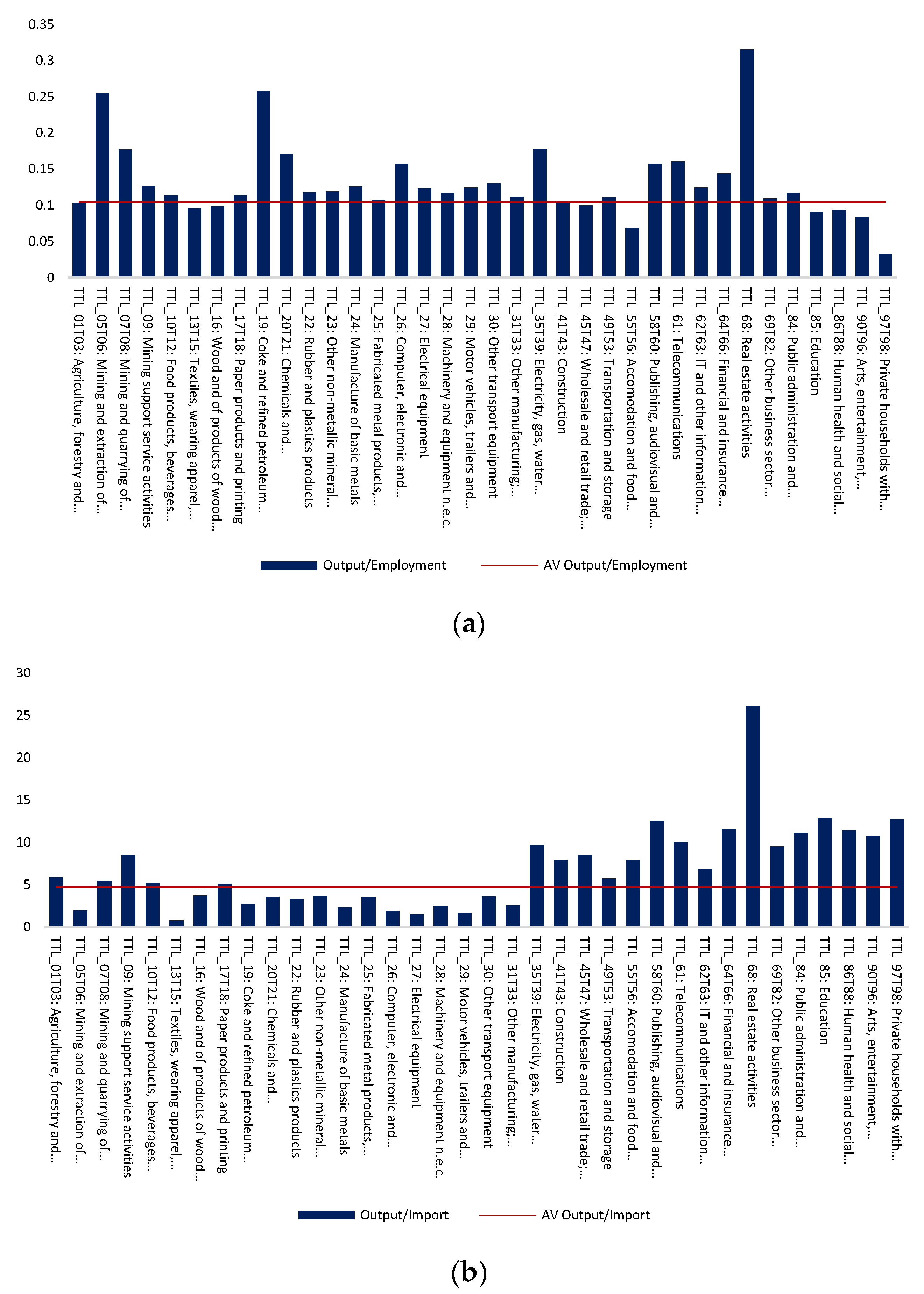
Figure 4, we observe that the incremental output-employment (output-import) ratio for primary production and industry is above (below) the economy’s average, while for services the opposite is true. However, if we estimate the incremental output-employment and output-import at the level of the 36 sectors, we observe that most of the sectors that are characterized by a high incremental output-employment and/or high output-import ratio belong to services (
Figure 5).
For a detailed analysis,
Table 1 presents the sectors with the incremental output-employment and output-import ratios above the economy’s average. In other words, it presents the sectors that should be considered for a long-term structural policy in order to enhance productivity and reduce import dependency.
4. Economic Growth Drivers
A demand policy can be applied by government expenditures, investments, or exports. Therefore, it is important to decompose the elements of total demand and to study the multiplier effects of each component separately. In this regard, the available data from the OECD split total final demand into the government’s final consumption expenditure, (government hereafter), gross fixed capital formation (investments hereafter), and exports. (For the multiplier effects of tourism in the US economy, see Rodousakis and Soklis [
29].)
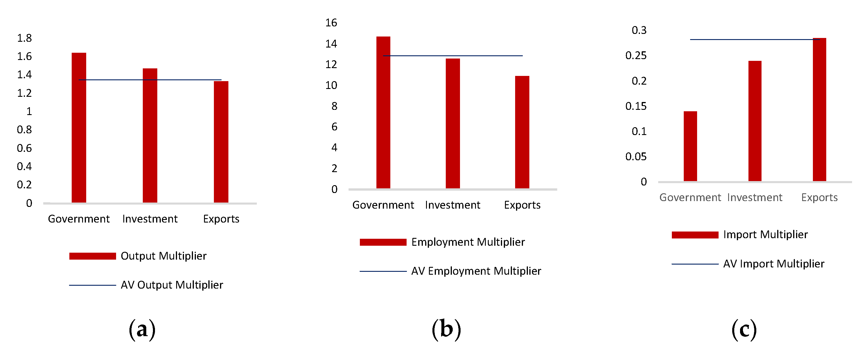
Figure 6 provides our estimation of the multiplier effects per category of the final demand of the US economy. It is observed that the government can be considered as the main agent for a demand policy. As there is, in the case of investments, a short distance between the employment multiplier and the economy’s average, we can also consider investments as an effective tool for boosting growth and employment.
Focusing now on the productivity indices and the import dependency indices per category of demand of the US economy, in
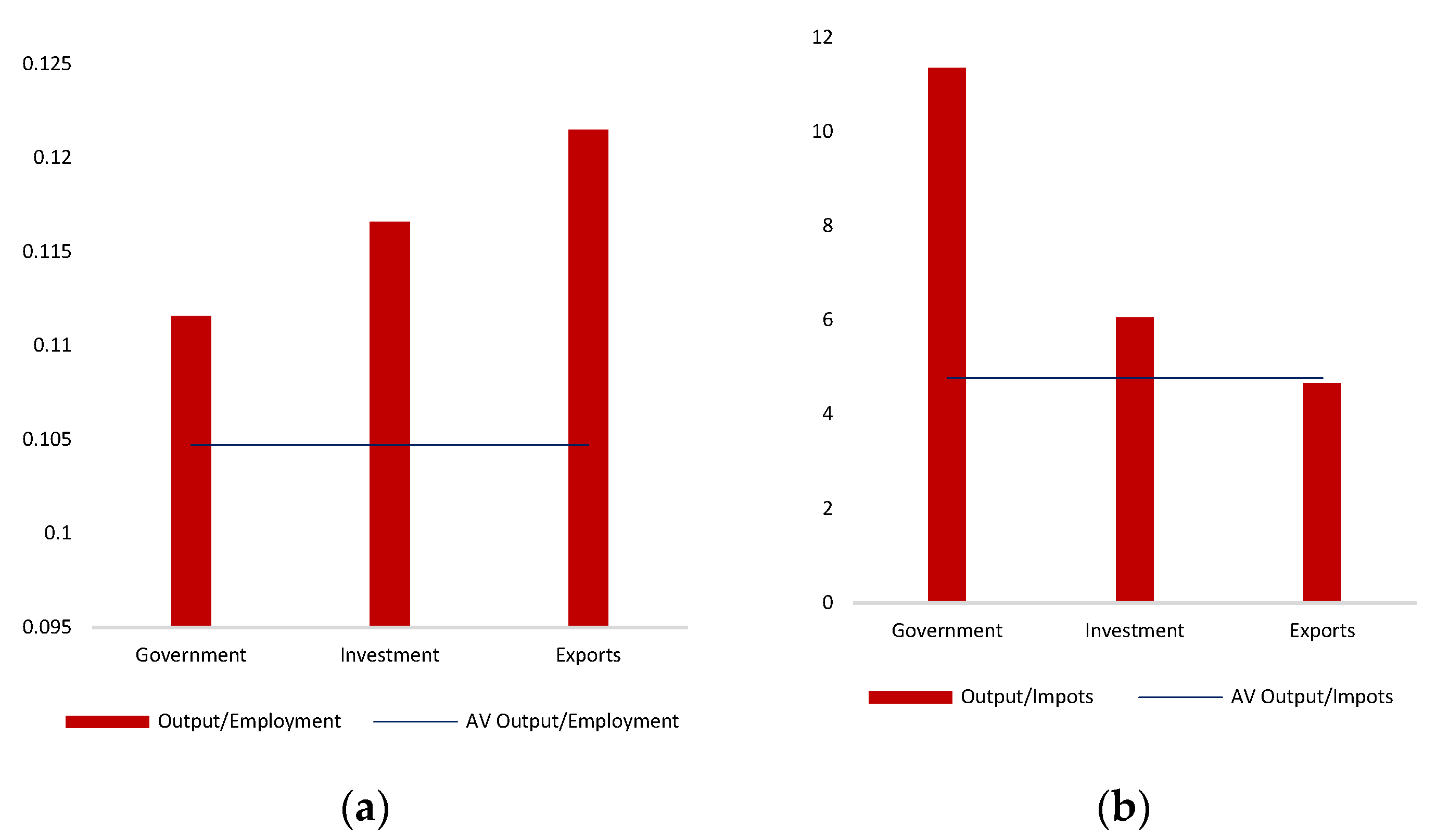
Figure 7 we present these indices for government expenditures, investment, and exports, as derived from our estimates presented in
Figure 6.
From
Figure 6, we observe that all the categories of final demand are characterized by favorable indices. (Note that for the exports the import dependency index is almost at the average levels.)
From the previous empirical findings, it follows that a short-term demand policy to boost economic growth for the US economy could be implemented through government spending and investments, as well as through exports. Furthermore, as all the sectors demonstrate a high incremental productivity index and low import dependency indices, this means that there is a great variety of short-term and long-term growth-oriented policies which can be adjusted accordingly to meet the challenges facing the US economy.
To conclude, the results of our analysis indicate that a change in government consumption spending by USD 1 million will cause:
A change in product output of about USD 1.64 million.
A change in employment levels of about 14.698 persons.
A change in the total imports of about USD 0.144 million.
Additionally, a change in investment by USD 1 million will cause:
A change in product output of about USD 1.47 million.
A change in employment levels of about 12.609 persons.
A change in total imports of about USD 0.242 million.
Finally, a change in exports by USD 1 million will cause:
A change in product output of about USD 1.33 million.
A change in employment levels of about 10.950 persons.
A change in total imports of about USD 0.285 million.
5. The Impact of the “American Jobs Plan and the American Families Plan”
In response not only to the COVID-19 pandemic-associated crisis but also to other significant problems in the US economy and society, many scholars have mentioned the necessity for a significant infrastructure plan and have shown that such a plan will also have significant benefits on a macroeconomic level (see, e.g., Papadimitriou et al. [
30]; Nikiforos and Zezza [
31]; and Papadimitriou et al. [
32]). In the same line, and mostly to increase the social cohesion of the US society, it also stressed the need for more education and health care. These proposals are relevant today because of the two main pillars of President Biden’s policy plan, i.e., “the American Jobs Plan and the American Families Plan”.
The first plan focuses on (re)building the aging infrastructures of the US. It is expected to utilize USD 2 trillion over a period of eight years. The second plan focuses on education, health care, and childcare. It recognizes that policies for the innovation and growth of tomorrow must focus on human capital and make life easier for American families. It is expected to utilize USD 1.8 trillion in a ten-year period.
This spending increase will be offset by corporate taxes, an increase on high-income households, and a reduction in the tax gap.
Considering the drivers of economic growth presented in the previous section, both plans are effective for short-term growth and job creation, as such a target could be implemented basically through government spending and investments. (The infrastructures correspond to a combination of “Construction” and “Other manufacturing; repair and installation of machinery and equipment”, while the education, health care, and childcare correspond to a combination of “Education” and “Human health and social work”). Furthermore, infrastructures are characterized by a high incremental productivity index and low import dependency indices and therefore are one of the best options for long-term growth-oriented policies, while the indexes for education and health are below average and therefore may not be the first choice for the implantation of such a long-term goal.
Based now on the multipliers of output, employment, and import for the 36 sectors of the US economy, the American Jobs Plan will cause a total increase in product output of about USD 2.81 trillion, while the American Families Plan will cause an increase of about USD 3.26 trillion.
The US GDP for 2020 reached USD 20.94 trillion and, therefore, from the previous analysis of the impact of the “American Jobs Plan and the American Families Plan” on the US economy, it is deduced that the USD 3.8 trillion is associated with a cumulative increase in output by almost 28 percent (USD 6.07 trillion) over a period of ten years. (The estimated cumulative financial costs of the COVID-19 pandemic related to the 3.4 percent decline in GDP.)
Of course, the purpose of this study is not a detailed evaluation of the American Jobs Plan and the American Families Plan, but it is, rather, to give an example of the usefulness of the multipliers estimation. Based now on the analysis of the properties of the US economy, one can design a number of alternative policy scenarios in order to achieve its multiple policy goals, namely to increase output and employment while taming imports. It can then be tested on several alternative policy scenarios based upon different compositions of the expenditure. i.e., picking ex ante the sectors in which to invest to deliver (a) the best growth results, (b) the best results in terms of employment, (c) the results that boost the productivity, and (d) the optional sector to control the import dependency, as well as to find (e) the “optional” sectors to combine the cases (a)-(d). Hence, the multipliers and the productivity import dependency indexes from the authorities can be used to test several alternative policy scenarios.
Finally, in the case of the availability of the necessary data, the multiplier effects brought by changes in the components of autonomous demand following the analytical budget expenditures can be explored. An example of this is the detailed evaluation per component of expenditure (i.e., 106 different investments expenditures) of the Greek Recovery and Resilience Plan (RRP) for the period of 2021-26, see [
33].
Last but not least, it should be mentioned that the proposed intersectoral analysis does not take into account the role of reforms which can in some cases change the structure of the economy and therefore the empirical evidence. This may be considered as the main weakness of our policy recommendations.
6. Concluding Remarks
The COVID-19 health crisis has affected the US economy dramatically. To alleviate this effect, policy makers, on the one hand, are trying to determine the sectors that should be considered for long-term policy to enhance productivity and reduce import dependency and, on the other hand, are highlighting the most effective policy response by considering output, employment, and import multipliers. Our research is based on an advanced input–output model which, except for the technical conditions of production, takes into account imports, income distribution, savings, and consumption patterns. The findings suggest that a change of USD 1 million in demand causes an average change of USD 1.35 million in product output, a change of 12.87 persons employed in production, and a change of USD 0.28 million in imports, while there is a wide range for deferment sectoral policies that allow concrete measurements of the concrete situation.
In general, the main proposal for the US policy makers is that the short-term policies to boost economic growth could be based on construction and services, while, judging in terms of the components of GDP, the most effective tools for implementing such a policy are the public consumption expenditures, investments, and exports. On the other hand, our long-term proposal to enhance productivity and reduce import dependency can take place through mining, food products, energy, public administration services, telecommunication, and logistics, among others. Judging now in terms of the components of GDP, a long-term policy plan could be based again on public consumption expenditures, investments, and exports. Hence, it is confirmed that there is a great variety of short-term and long-term policies that can be adjusted according to the circumstantial challenges of the US economy. (As a counter-example to the policy proposals of this paper for the US economy, we could refer to the case of the Greek economy, in which the application of the current analysis [
24] indicated that a short-term growth-oriented policy could be implemented basically through the service sector, while the fact that the sectors that are characterized by the highest productivity exhibit at the same time the highest import dependency index, implies that the policy makers have to deal with an impossible puzzle.)
Thus, the current analysis provides an analytical view of the structure and the interrelationships of the US economy, and therefore, policy makers can choose from a variety of alternative policy plans the most appropriate to achieve the recovery or/and resilient goals set by the authorities. We could have constructed different examples for a post-COVID-19 program; however, we evaluated the already announced plans in order to assess the impact of the post-COVID-19 policies under implementation. Hence, we estimate the impact of the recently announced infrastructure and families plans, of which the size is about USD 3.8 trillion for a ten-year period. It was found that these programs are associated with a cumulative increase in output by almost 28 percent, i.e., these plans are able to ensure a strong growth for the US economy for the next ten years. All of the above suggest that addressing the impact of the pandemic requires planning and targeted sectoral policies and, furthermore, show that a government spending program based on infrastructures and education would have a significant positive impact on the US economy and society, ensuring impressive macroeconomic benefits. Of course, the current analysis does not consider the implications of unpredictable events such as the recent Ukrainian crisis. Such an event can of course have an impact on imports and exports, as well as on the structure of the economy, which could significantly alter the estimated effects of this study. Another limitation of our analysis is that we do not take into account the role of reforms and how they can also affect our results. However, the knowledge of the structural capabilities of the US economy offered by this study can easily incorporate alternative scenarios caused by unforeseen shocks, such as a pandemic and/or a war.
