Experimental Study on the Carbon Sequestration Benefit in Urban Residential Green Space Based on Urban Ecological Carrying Capacity

Abstract

The CO₂ concentration of urban residential green space in Changsha was experimentally investigated. Based on the experimental results, the variation characteristics and influencing factors of CO₂ concentration in residential areas were analyzed considering both the measuring time and ecological plant structure. Then, through the concept of urban ecological bearing capacity, the carbon sequestration index of the urban residential areas was proposed in this paper. Finally, the regulating effects of varieties of vegetation on CO₂ concentration among four urban residential areas were deeply analyzed and discussed. Results showed that green space with an ecological plant structure of trees-shrubs-grass exhibited greater improvement in the environmental carbon balance than those of shrubs or grass, and the atmospheric carbon sequestration capacity was significantly affected by the total quantity of the green space.

1. Introduction

The urban residential areas, as an essential component of ecosystem, have become a topic of everlasting interest to researchers and practitioners. In order to maintain the sustainable development of the urban residential areas, during the preceding decades, much effort has been directed towards the exploration on the ecological environmental bearing capacity of the green spaces [1,2], the coupling effects of human activities and variations of natural ecological environment [3], as well as the environmental amenity in urban residential areas [4,5]. Recently, due to the unceasing acceleration of global climate change (also known as the greenhouse effect) induced by the uncontrolled emission of CO₂ and other greenhouse gases [6], the concept of low-carbon development has been treated as the main theme on the topic of sustainable development in urban residential areas around world [7,8].

So far, in order to mitigate the greenhouse effect, a number of countries have introduced several limitation targets against carbon emissions to aim to achieve efficient carbon sequestration. For example, China has pledged to achieve the target of carbon neutrality by 2026. In detail, the main components of the greenhouse gases are H₂O, CO₂, CH₄, and CO. Specifically, the main route of the carbon cycle can be demonstrated as follows: CO₂ from atmosphere is firstly absorbed by land and marine plants, then returned to the atmosphere through biological and geological processes and human intervention. During this cycle, the effects of CH₄ and CO are relatively moderate when compared with CO₂ [9,10]. Due to the fact that H₂O is usually not affected by human activities and CO is an indirect element, the CO₂ can be treated as the most contributing factor that enhances the greenhouse effect [10]. Therefore, a number of countries have conducted a series of programs to monitor the urban atmospheric CO₂ concentration [10,11,12].

At present, since most research regarding carbon sequestration mainly focuses on the bearing capacity of land, forests, lakes, and other large-scale spaces, the studies on smaller-scale green spaces are limited. For example, Rowntree and Nowak [13] estimated the carbon storage of urban forests in the United States, then analyzed the carbon absorption for urban green space and the reduction effect on carbon emission caused by human activities in two cities; Idso et al. [14,15] studied the distribution of near-surface atmospheric CO₂ concentration in Phoenix based on the inverse distance weight interpolation method and indicated that the concentration was significantly higher before sunrise than that of middle of day, and the causes were concluded to be the coupling effects of the atmospheric vertical mixing and vegetation photosynthesis; Wentz et al. [16] addressed the correlations among near-surface atmospheric CO₂ concentration, urbanization level (in terms of population, average traffic flow, and employment), and the vegetation coverage rate based on mobile monitoring data with regression analysis; Henninger et al. [17] studied the near-surface atmospheric CO₂ concentration in Essen based on mobile monitoring data, and the results showed that there were significant variations in different measuring areas and times for the concentration, and the average value in cities was 8.9% higher than that in suburbs. In addition, the research also found that the concentration variation was greater in winter when compared with summer, which resulted from the seasonal alterations in carbon emissions, the efficiency of the vegetation photosynthesis, and atmospheric conditions.

Concretely, with the continuous improvement of residents’ living conditions, green plants have been treated as an indispensable component for the construction of modern urban residential areas [18,19,20,21,22,23,24,25]. For instance, Liang [21] studied the greenhouse effect by focusing on the green plants in residential areas and pointed out that the special physiological process of green plants, including carbon fixation and oxygen releasing, can contribute to the mitigation of the greenhouse effect. Meanwhile, in order to achieve eco-friendly and low-carbon development in both urban and rural areas, several countries have also issued a series of guiding documents specific to green plants [26,27,28].

According to previous studies, most researchers believed that the ecological environmental benefits resulting from the carbon sequestration of green plants were chiefly dependent on the efficient areas of leaves for completing the photosynthesis. Such benefits were usually determined by measuring the green quantity in certain regions [29,30,31,32], and plant carbon sequestration ability was generally calculated based on the relative biomass [33]. Hence, in this research, the CO₂ concentration is treated as the main operable factor for evaluating the effect of greenhouse gas on the urban ecological environmental condition. The relationship between the quality of the green space and the ecological environmental bearing capacity will be analyzed based on the measurement of CO₂ concentration in several sampling points.

Therefore, based on the above assertions, the main objective of the current research is to investigate the effects on the CO₂ concentration resulting from measuring time, location, and the plant community structure of the green spaces in urban residential areas. It is believed that the results can provide a theoretical basis and practice support for planning and constructing green spaces in order to efficiently improve the ecological environment in urban residential areas.

2. Materials and Methods

2.1. Observation Sites Setup

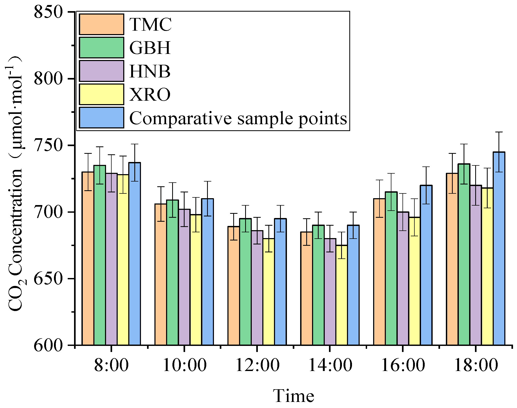
The observation sites were set up in four urban residential communities, which were located in the North (Xiangjiang River One and Huasheng New Band, aka XRO and HNB, respectively), central (Tongtai Meiling Court, aka TMC) and South (Ginkgo biloba home, aka GBH) areas of Changsha City in China, respectively. Specifically, in those communities, the plant spaces were all constructed after 2007, so the comparability for relevant analysis can be guaranteed. All sampling points were set up in accordance with the principle of randomness and uniformity and arranged in intersection points with help of GPS positioning. Meantime, the locations of these sampling points were fine-tuned according to the plant community structure of the green spaces. The detailed information of the plant community structure is listed in

Table 1. Plant community structure of green spaces and vegetation coverage.

Green Space Type	Vegetation Coverage (%)
	Trees	Shrubs	Grass
Trees-Shrubs-Grass	70	50	50
Shrubs-Grass	30	80	20
Lawn	30	40	60
Trees	100	0	0
Shrubs	0	100	0
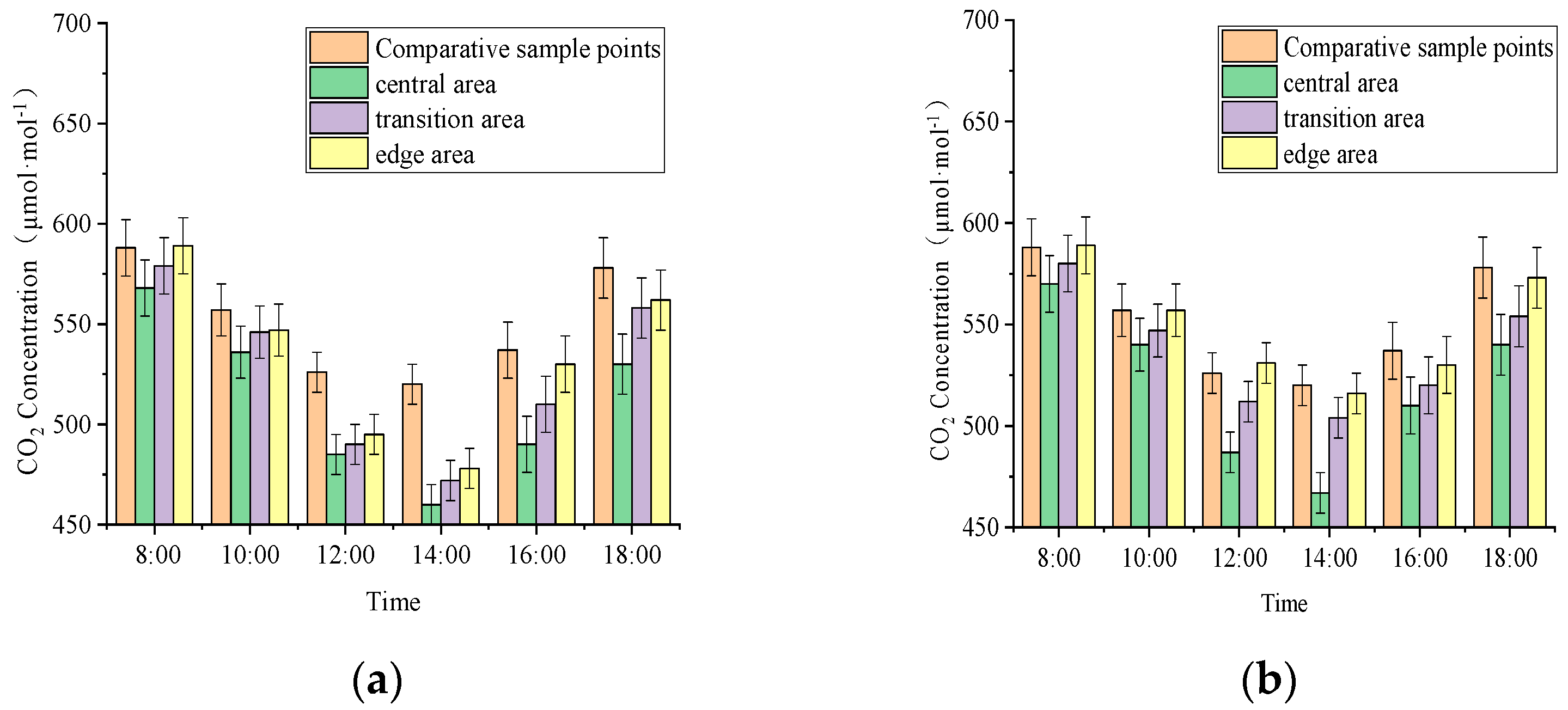
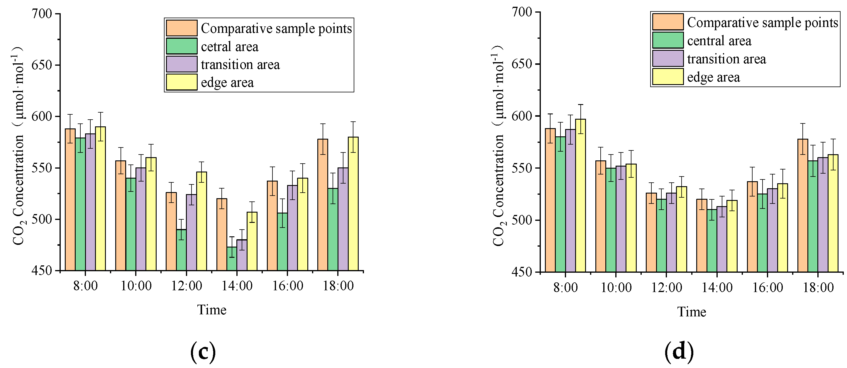
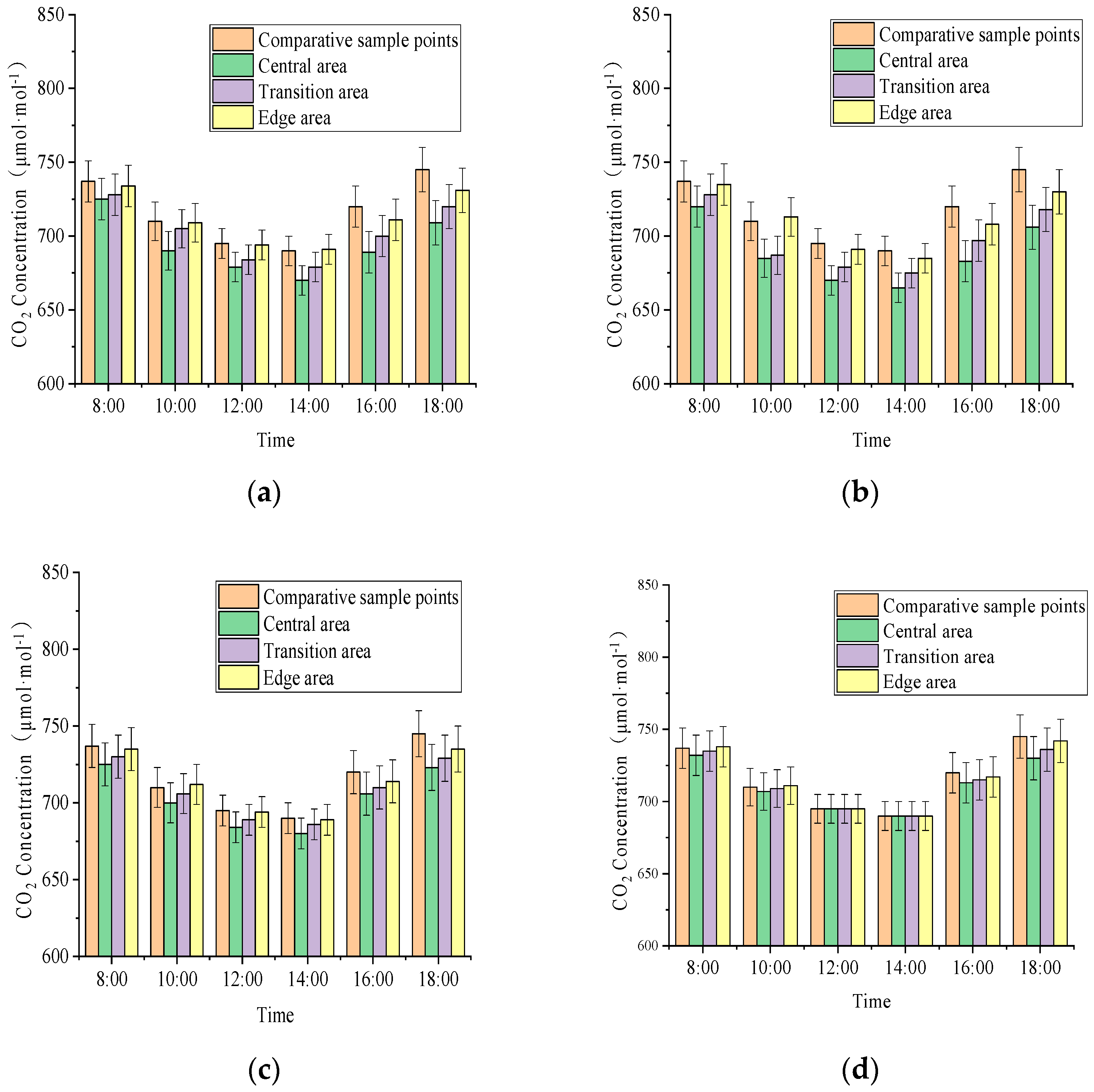
Grass	0	0	100

. In addition, in order to obtain the spatial gradient of CO₂ concentration in the urban residential areas, for each observation site, the measuring areas were separated into central zone, transition zone, and edge zone.

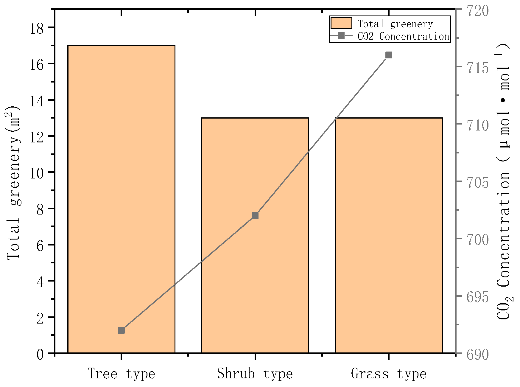
Concretely, the ground green space chiefly consisted of shrubs, grass, and the trunks of trees. Therefore, the total green quality in this research is determined as the sum of the areas of the shrubs, grass, and the vertical projection of trees. Additionally, by considering the overlapping effect of the above-mentioned areas, the value of the vegetation coverage for the different varieties of vegetation can be eventually obtained.

Moreover, the bearing capacity of residential green space refers to the ability of the ecosystem to maintain its normal operation under various conditions. The relative bearing capacity index (also known as bearing capacity index ratio) is generally determined by the ratio of the measured value for ecosystem’s bearing capacity and the critical value for that in certain conditions. Specifically, when the bearing capacity index ratio is larger than 1, it indicates that the pressure of the whole ecosystem in the region is greater than the standard, and the ecosystem can no longer bear economic activities. When the bearing capacity index equals 1, it indicates that the pressure generated by the residential economic activities of the residential green ecosystem is equal to the supporting force of the system, which is within the bearing capacity range. When the bearing capacity index is less than 1, it indicates that the pressure faced by the ecosystem does not exceed the maximum value it can bear, and the threat brought by the economic activities of residents in the community has not caused a relatively obvious impact, so the overall ecosystem tends to develop healthily. When the number of impact factors becomes lower, the ecosystem effect will be better, and people will feel more comfortable and work more efficiently.

After the geographical positions of the sampling points were determined, measuring instruments were placed in the center of each point. Additionally, the canopy density and plant community structure were measured. In this research, the average CO₂ concentrations from two comparison sample points were treated as the background data of the ecological environment for the urban residential areas. In detail, the comparison sampling points were located on the east side of GBH and HNB, with a small number of surrounding green landscape environments, respectively. The detail information for the sampling points is listed in

Table 2. Basic information of sample points in residential green space.

Sample Point	Location	Plant Community Type	Canopy Density
Comparison sample point 1	112°98′73″ E, 28°14′65″ N	-	-
Comparison sample point 2	112°98′30″ E, 28°21′70″ N	-	-
A	112°96′59″ E, 28°29′96″ N	Trees-Shrubs-Grass	0.75
B	112°96′55″ E, 28°29′95″ N	Shrubs-Grass	0.45
C	112°96′55″ E,28°29′92″ N	Shrubs-Grass	0.45
D	112°98′14″ E, 28°21′71″ N	Trees-Shrubs-Grass	0.75
E	112°98′09″ E, 28°21′71″ N	Trees-Shrubs-Grass	0.75
F	112°98′05″ E, 28°21′73″ N	Shrubs-Grass	0.45
G	112°99′88″ E, 28°14′46″ N	Trees-Shrubs-Grass	0.75
H	112°99′88″ E, 28°14′46″ N	Shrubs-Grass	0.45
I	112°99′88″ E, 28°14′46″ N	Lawn	0.30
J	112°98′82″ E, 28°14′57″ N	Lawn	0.30
K	112°98′86″ E, 28°14′57″ N	Lawn	0.30
L	112°98′89″ E, 28°14′57″ N	Lawn	0.30

.

2.2. Measurements Method

In this research, the instrument for measuring the CO₂ concentration is Bohu intelligent CO₂ detector. It is based on gold-plated infrared photoconductivity technology and capable of automatic calibrating with a measurement accuracy of ±30 ppm. During the measuring process, the self-contained software of the instrument was used to record CO₂ concentration data per 60 s due to its sampling response time.

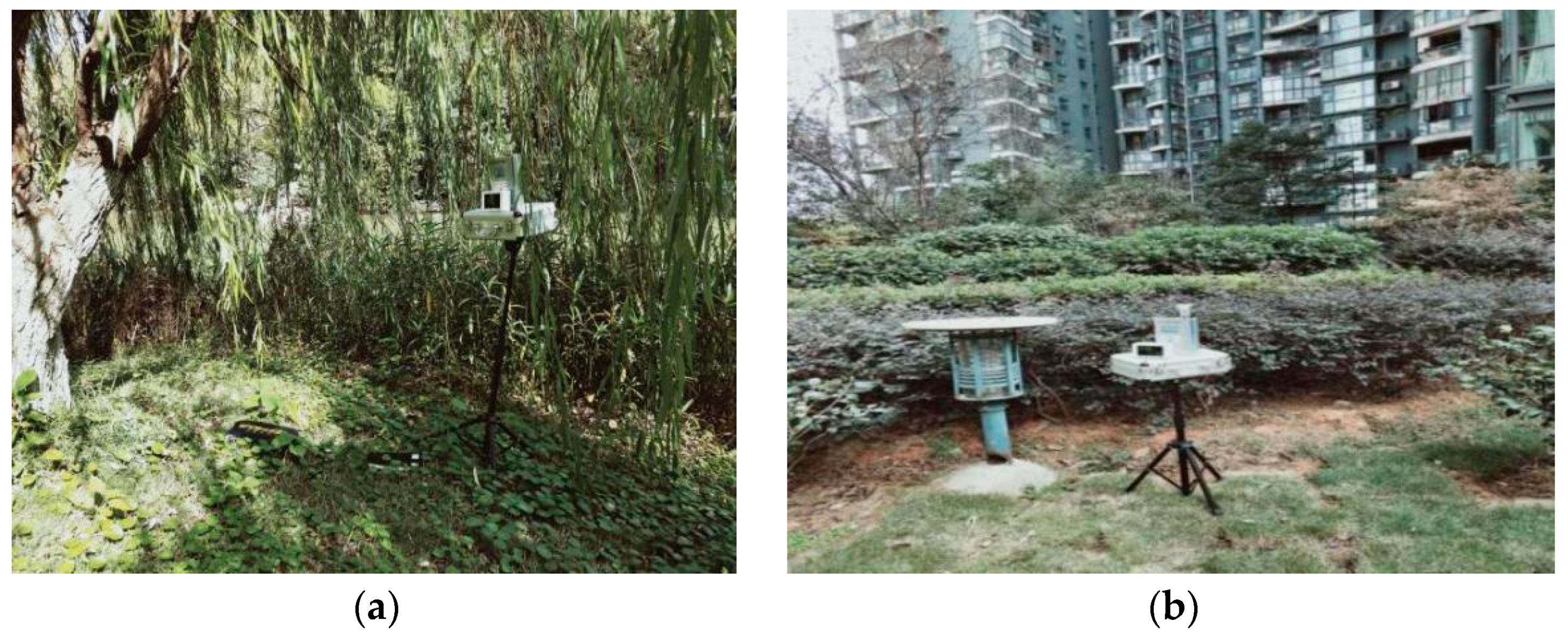
In order to guarantee the measured results are representative of spatio-temporal and ecological benefit factors, in this research, the measurements were conducted on a day when meteorological conditions and the weather conditions were relatively stable. During the measuring process, the instrument was kept within a certain distance from the ground (generally 1.4 m, and the monitoring time ranged from 8:00 to 18:00), as shown in Figure 1. To avoid the influences of atmospheric temperature and humidity, data collection was carried out within an interval of two hours with a detection time of 5 min.

Moreover, in order to obtain the annual variation of CO₂ concentration in urban residential green space, monthly measurements of CO₂ concentration were also conducted between the 20th and 25th from May 2019 to May 2020. During the data analysis process, the average value of measured CO₂ concentration of sample points was compared individually to indicate the environmental background data of the urban residential areas.

After obtaining the measuring data, the two-way and one-way variance analysis was conducted on the diurnal variation of measured CO₂ concentration based on difference method by considering the monthly variation and plant community structures, which was attempted to examine the influences resulting from both the measuring time and the location. In detail, relevant calculation methods are shown in

Table 3. Variance analysis of regional samples and time CO₂ concentration of urban residential green space.

	Quadratic Sum	Degree of Freedom	Mean Square	Mean Square Percentage	Probability (α = 0.05)
	SS	DF	MS	F	P
Location	$S_A^2=\mathrm{sm}{\displaystyle \sum _{i=1}^r(\overline{X_i}}-\overline{X}{)}^2$	$r-1$	${\overline{S}}_A^2=\frac{S_A^2}{r-1}$	$F_A={\overline{S}}_A^2/{\overline{S}}_E^2$	$P_A=P(F_A>F_{1-p_A})$
Error	$S_E^2={\displaystyle \sum _{i=1}^r{\displaystyle \sum _{j=1}^s{\displaystyle \sum _{k=1}^m(X_{ijk}}}}-{\overline{X}}_{ij}{)}^2$	$r\mathrm{s}(m-1)$	${\overline{S}}_E^2=\frac{S_E^2}{rs(m-1)}$	/	/
Time	$S_B^2=\mathrm{rm}{\displaystyle \sum _{j=1}^r(\overline{X_j}}-\overline{X}{)}^2$	$s-1$	${\overline{S}}_B^2=\frac{S_B^2}{s-1}$	$F_B={\overline{S}}_B^2/{\overline{S}}_E^2$	$P_B=P(F_B>F_{1-p_B})$
Error	$S_E^2={\displaystyle \sum _{i=1}^r{\displaystyle \sum _{j=1}^s{\displaystyle \sum _{k=1}^m(X_{ijk}}}}-{\overline{X}}_{ij}{)}^2$	$r\mathrm{s}(m-1)$	${\overline{S}}_E^2=\frac{S_E^2}{rs(m-1)}$	/	/

and

Table 4. One-way ANOVA of monthly and seasonal CO₂ concentration of urban residential green space.

Quadratic Sum	Degree of Freedom	Mean Square	Mean Square Percentage	Probability (α = 0.05)
SS	DF	MS	F	P
$S_E^2={\displaystyle \sum _{i=1}^r{n}_i}{(\overline{Y_i}-\overline{Y})}^2$	$r-1$	${\overline{S}}_A^2=\frac{S_A^2}{r-1}$	$F=\frac{{\overline{S}}_A^2}{{\overline{S}}_E^2}$	P
$S_E^2={\displaystyle \sum _{i=1}^r{\displaystyle \sum _{j=1}^{n_i}(}}\overline{Y_{ij}}-\overline{Y_i}{)}^2$	$n-r$	${\overline{S}}_E^2=\frac{S_E^2}{n-r}$	/	/
$S_E^2={\displaystyle \sum _{i=1}^r{n}_i}{(Y_{ij}-\overline{Y})}^2$	$n-1$	/	/	/

, respectively.

Where $r$ is the level number of factor A, that is, the number of months and seasons; n is the total number of samples, $\overline{X}$ denotes the mean of samples, n_j denotes the number of repeated experiments under the level A_j, X_i is the average CO₂ concentration under the level A_j (month and season), and X_ij is the CO₂ concentration in the jth region in the ith month or season

3. Results and Discussion

3.1. Diurnal and Gradient Variations of CO₂ Concentration in Urban Residential Green Space

(1) CO₂ concentration in urban residential green space during plant growing season.

The CO₂ concentration in the urban residential green space of the sampling points firstly exhibits a significant decreasing trend from 8:00 AM to 14:00 PM followed by a boom up until 18:00 PM (Figure 2). The maximum daily variation of the sample points and the comparison sample points are 118 μmol·mol⁻¹ (occurred in XRO) and 68 μmol·mol⁻¹, respectively. Additionally, there is a significant difference in the CO₂ concentration during the changes of the measuring times and locations. It is also noted that among the four measured urban residential communities, the highest to the lowest measured CO₂ concentrations occurred in GBH, TMC, HNB, and XRO, respectively.

In addition, the CO₂ concentration of sample points in the core zone for each urban residential community are all less than those in the transition zone and the edge zone (Figure 3). The variation trend of CO₂ concentration in the comparison sample points are similar to those in the four urban residential areas. However, it is note-worthy to stress that for the comparison sample points, the variation range is lower than that measured in the core area, which is 68μmol·mol⁻¹.

Specifically, in Figure 2, it is observed that the for all sampling points, the CO₂ concentration are gradually declined between 8:00 a.m. to 12:00 a.m. After the CO₂ concentration reached the lowest point at 14:00 PM, the values tended to increase slowly.

By comparing the CO₂ concentration in different locations during the plant growth season, it can be found that for all the locations, including the core, transition, and edge zones, the CO₂ concentrations are increasing significantly. Moreover, although both the measuring locations and the times can impact the CO₂ concentrations, different measuring times will cause greater changes in CO₂ concentration (

Table 5. Regional samples and variance analysis of CO₂ concentration in the growth season of urban residential green space.

	Quadratic Sum	Degree of Freedom	Mean Square	Mean Square Percentage	Probability (α = 0.05)
	SS	DF	MS	F	P
Location	11,542.61	3	3847.54	16.15	5.76 × 10−4
Error	2144.76	9	238.31	/	/
Time	79,906.97	5	15,981.39	143.39	4.11 × 10−12
Error	1671.82	15	111.45	/	/

).

(2) CO₂ concentration in urban residential green space during plant non-growing season.

The overall change pattern shows a trend of decreasing first and subsequent increasing, which is similar to the corresponding change result in the plant growing season (Figure 4). In addition, the CO₂ concentration at all sample points are higher than those measured during the growing season.

According to Figure 5, it is demonstrated that the variating trend of the measured CO₂ concentration during 8:00–12:00 in the plant non-growing season is similar to that of growing season (Figure 5). In detail, the measured results for all the sampling points displayed a trend of firstly increasing before 14:00 PM and then declining. Compared with core and the transition zones, the largest decreases were found in the edge zone.

It is also worth stressing that when compared with the measurement location, the measuring time yields a more significant impact, and the overall influence is lower in the plant non-growing season than in the plant growing season (

Table 6. Analysis of variance of CO₂ concentration in non-growing season regional samples and time of urban residential green space.

	Quadratic Sum	Degree of Freedom	Mean Square	Mean Square Percentage	Probability (α = 0.05)
	SS	DF	MS	F	P
Location	4218.13	3	1406.04	11.10	0.002
Error	1140.46	9	126.72	/	/
Time	32,113.88	5	6422.78	521.12	2.94 × 10−16
Error	184.88	15	12.33	/	/

).

3.2. Monthly Variation Characteristics of CO₂ Concentration for Green Space Plants in Residential Area

The monthly average CO₂ concentration and the relative analysis of variances from May 2019 to May 2020 are illustrated in Figure 6 and

Table 7. Variance analysis of monthly CO₂ concentration of regional sample points in urban residential green space.

	Quadratic Sum	Degree of Freedom	Mean Square	Mean Square Percentage	Probability (α = 0.05)
	SS	DF	MS	F	P
Inter-group	614,779.65	11	55,889.06	89.88	0
Intra-group	29,848.00	48	621.83	/	/
Sum	644,627.65	59	/	/	/

, respectively. From Figure 6, it is observed that significant diversities occurred in different measured locations. Specifically, the highest CO₂ concentrations were found in November, December, and January. In detail, in December, the average CO₂ concentration of GBH reached 718 μmol·mol⁻¹, while that obtained from a comparison sampling point is 720 μmol·mol⁻¹. The measurement results of CO₂ concentrations in May, June, July and August were comparatively low. For example, the average minimum CO₂ concentration of XRO in July was 400 μmol·mol⁻¹, and that of the comparison point was 490 μmol·mol⁻¹. Moreover, the monthly average CO₂ concentration measured from the sampling points were lower than the comparison sampling points. In Table 7, it was found that there were significant changes in CO₂ concentration gradients in terms of months with different measured locations (Table 7).

3.3. Seasonal Variation Characteristics of CO₂ Concentration in Residential Green Space

It was found that the CO₂ concentration varied significantly in different seasons (Figure 7). In detail, the corresponding location and season with the lowest value were found to be XRO and summer, with an average value of 450 μmol·mol⁻¹, which is lower than the comparative sampling point, 501 μmol·mol⁻¹. Moreover, the CO₂ concentration for all sampling points only presented a small difference in winter, and the measured values of the sampling points were all smaller than those of the comparison sampling points. The results of seasonal variance analysis are listed in

Table 8. Variance analysis of CO₂ concentration in different seasons of regional samples in urban residential green space.

	Quadratic Sum	Degree of Freedom	Mean Square	Mean Square Percentage	Probability (α = 0.05)
	SS	DF	MS	F	P
Inter-group	159,529.20	3	53176.40	165.34	2.99 × 10−12
Intra-group	5146.00	16	321.63	/	/
Sum	164,675.20	19	/	/	/

.

3.4. CO₂ Concentration and Plant Community Structure of Urban Residential Green Space

As can be seen from

Table 9. Plant community structure and CO₂ concentration in residential green space (μmol·mol⁻¹).

Types of Plant Community Structure	Sample Point	Concentration of CO2 (μmol·mol−1)
Comparison sample points 1	/	725	724
Comparison sample points 2	/	723
Trees-shrubs-grass type	A	685	692.25
	D	695
	F	696
	G	693
Shrubs-grass type	B	700	702.5
	C	703
	E	705
	H	702
Lawn type	I	713	716
	J	717
	K	714
	L	720

, among all the measured sampling points, the lowest value of CO₂ concentration occurred in the plant community structure of trees-shrubs-grass with 692.25 μmol·mol⁻¹, while the highest value emerged in the plant community structure of lawn with 720 μmol·mol⁻¹. For the plant community structure of shrub-grass, the value of the CO₂ concentration was 702.5 μmol·mol⁻¹. Notably, according to the variance analysis in

Table 10. Variance analysis of CO₂ concentration of plant structure types of regional samples in urban residential green space.

	Quadratic Sum	Degree of Freedom	Mean Square	Mean Square Percentage	Probability (α = 0.05)
	SS	DF	MS	F	P
Inter-group	1849.75	3	616.58	51.49	2.19 × 10−6
Intra-group	119.75	10	11.98	/	/
Sum	1969.50	13	/	/	/

, it was revealed that the CO₂ concentrations of the varied community structures experienced significant differences.

3.5. Analysis of the Relationship between Total Amount of Residential Green Space and CO₂ Concentration and Ecological Bearing Capacity

3.5.1. The Relationship between the Total Green Quantity of Residential Green Space and CO₂ Concentration

Residential green space is mainly composed of trees, shrubs, and grass. Considering the existence of trees in the ground space that mainly in the form of trunks, the ground green space is mainly composed of the shrubs and grass. In this research, the total green quantity is represented by the sum of grass (A_lawn), shrubs (A_shrub) and vertical projection area of the tree crowns (A_a1) in residential green space, which can be calculated by

$$A_{totalgreenquantity}=A_{lawn}+A_{shrub}+A_{al}$$

(1)

Considering the overlapping effects of above components, the minimum and maximum value of the greening volume ratio (R_g) are assumed to be 0 and 2 in this research, respectively, and it can be evaluated by the ratio between the summation of the areas of grass (A_lawn), shrubs (A_shrub), and the tree crowns (A_tree) on the total green quantity (A_{green space}), such as

$$R_g=(A_{lawn}+A_{shrub}+A_{tree})/A_{greenspace}$$

(2)

Table 11. Plant areas, total green quantity, and green capacity in sample points area of residential green space.

Residential Communities	Area of Total Green Space (m2)	Trees (m2)	Shrubs (m2)	Grass (m2)	Total Green Quantity (m2)	Greening Volume Ratio
GBH	5269	1580.7	2107.6	3161.4	6849.7	1.3
TMC	5589	2828.3	3543.1	2045.9	8417.3	1.5
HNB	6677	4036.7	3220	3457	10,713	1.6
XRO	6720	4060.2	3683.8	3036.2	10,780	1.6

shows the calculation results of different varieties of vegetation, plant areas, total green quantity, and greening volume ratio from the sampling points in urban residential green space:

Plants can significantly reduce the concentration of CO₂ in the ecological environment, which is imperative for the achievement of carbon and oxygen balance in cities. As can be seen from Figure 8, the greater the total green number of plants in residential areas, the higher the carbon sequestration amount and the lower the CO₂ concentration. In addition, the total amount of trees is the main factor that reflected the total amount of green per unit area, which contributed more to the total amount of green than shrubs and grass. Moreover, in regard to the total green quantity, the green plot ratio reflects the quality of green space. The lower the CO₂ concentration, the larger the green area or the higher the green area ratio. In terms of carbon sink of urban residential green space, vegetation in residential green spaces is the main part of fixed and accumulated CO₂. The influencing factors of plant carbon sequestration capacity mainly include vegetation species, growth years, and community structures. In addition, environmental climate, external disturbance, vegetation coverage, and layout rationality can certainly affect the carbon sequestration ability of plants as well.

Specifically, it can also be observed in Figure 9 that the highest to lowest carbon sequestration capacities for different varieties of vegetation are trees > shrubs > grass.

3.5.2. Analysis of the Relationship between Total Green Quantity and Bearing Capacity of Residential Green Space

The classification of environmental bearing capacity of residential green space is shown in

Table 12. Classification standards of CO₂ bearing capacity of urban residential green space.

Capacity Evaluation Value	Description
evaluation value > 3.0	excessive overload
1.0 < evaluation value < 3.0	overload
evaluation value = 1	full load
0.7 < evaluation value < 1.0	reasonable bearing
evaluation value < 0.7	well bearing

, and the calculation value can be divided into excessive overload, overload, full load, reasonable bearing capacity, and good bearing capacity.

The actual bearing capacity of residential green space to CO₂ concentration is determined by the maximum number of pollutants it can accept. Small amounts of CO₂ will not pose a threat to human survival, but if human beings and other organisms inhale too much CO₂ in a short period of time, it will cause different level of risk. The relationship between CO₂ concentration and human comfort is shown in

Table 13. CO₂ concentration versus human comfort.

Degree	Human Discomfort Symptoms at Different CO2 Concentrations	Symptom
1	350–400 μmol·mol−1	Healthy
2	400–700 μmol·mol−1	Normal level
3	700~1000 μmol·mol−1	Acceptable
4	1000–200 μmol·mol−1	Tired and discomfort
5	2000–4000 μmol·mol−1	Dyspneic

:

As can be seen from the above table, the critical value of CO₂ concentration for human comfort is 700 ppm.

For the index of capacity R_i, it can be calculated as following equation and the calculated results are listed in

Table 14. Index of bearing capacity of green space in each residential area.

	XRO	HNB	TMC	GBH
Index of bearing capacity	0.78	0.8	0.81	0.82
Degree of bearing	Reasonable bearing	Reasonable bearing	Reasonable bearing	Reasonable bearing

$$R_i=C_i/C_{i0}$$

(3)

in which the R_i denotes the index of capacity (refers to relative occupancy ratio of CO₂ concentration on ecological environmental bearing capacity; C_i is the measured result of the CO₂ concentration; C_i0 is the critical value of the CO₂ concentration, which can be directly obtained from Table 13; when R_i is less than 1, the degree of ecological environmental bearing capacity is overloading.

Results in Table 14 reveals that the green space of the four residential areas studied in this paper are in a reasonable bearing state at present and fall short of the requirements of well bearing capacity. Therefore, the bearing capacity of the corresponding residential green space to CO₂ concentration can be improved by increasing a certain area of ecologically complex green spaces of trees-shrubs-grass.

4. Conclusions

In this paper, experimental investigations of CO₂ concentration in typical urban residential communities were reported. By taking into account the ecological carbon sequestration capacity of green spaces, its benefits and efficiencies were explored by dint of analyzing several dominant influence factors, including total green quantity, location, and plant community structure. The key conclusions can be drawn as follows:

(1)

The CO₂ concentration in urban residential area is essentially dependent on the location, measuring time, and plant community structure of the green space. The total green quantity has a positive correlation with carbon sequestration capacity;

(2)

The maximum and minimum CO₂ concentrations emerged in winter and summer, respectively. Such seasonal variations were attributed to human activities and plant phenology in urban residential communities;

(3)

Plant community structures with trees-shrubs-grass had the highest carbon sequestration capacity compared with other types. In same ground area, ecologically complex green spaces containing shrubs, trees and grasses performed much better than simple green spaces only containing single plant species such as grass;

(4)

The green spaces in urban residential areas studied in this paper were all in the degree of reasonable bearing. In order to improve the local ecological environment, planning authorities could plant ecologically complex green spaces instead of the current plant community structures.

References

1. Verhulst, P.F. Notice sur la loi que la population suit dans sonaccroissement.Correspondance mathématique et physiquepubliée par A. Quetelet 1838, 10, 113–121. [Google Scholar]
2. Yan, H.; Wu, F.; Dong, L. Influence of a large urban park on the local urban thermal environment. Sci. Total Environ. 2018, 622, 882–891. [Google Scholar] [CrossRef] [PubMed]
3. Bishop, A.B. Carrying Capacity in Regional Environment Management; Government Printing Office: Washington, DC, USA, 1974.
4. Schneider, D.; Odschalk, D.R.; Xler, N. The Carrying Capacity Concept as a Planning Tool; American Planning Association: Chicago, IL, USA, 1978. [Google Scholar]
5. Baruch, G. Outdoor comfort research issues. Energy Build. 2003, 35, 77–86. [Google Scholar]
6. IPCC. Climate Change 2007: Mitigation of Climate Change; Cambridge University Press: Cambridge, UK, 2007. [Google Scholar]
7. Jenks, M.; Burton, E.; Williams, K. The compact city: A sustainable urban form. Urban Des. Int. 1996, 1, 293–294. [Google Scholar]
8. Levin, I.; Graul, R.; Trivett, N.B. Long-term observations of atmospheric CO2 and carbon isotopes at continental sites in Germany. Tellus B 1995, 47, 23–34. [Google Scholar] [CrossRef] [Green Version]
9. Geng, Y.B.; Dong, Y.S.; Memg, W.Q. Research advances on terrestrial carbon cycle. Adv. Geogr. 2000, 19, 297–306. [Google Scholar]
10. Xu, Q.; Dong, Y.X.; Yang, R. Influence of land urbanization on carbon sequestration of urban vegetation: A temporal cooperativity analysis in Guangzhou as an example. Sci. Total Environ. 2018, 635, 26–34. [Google Scholar] [CrossRef]
11. Idso, S.B.; Idso, C.D.; Balling, R.C., Jr. Seasonal and diurnal variations of near-surface atmospheric CO2 concentration within a residential sector of the urban CO2 dome of Phoenix, AZ, USA. Atmos. Environ. 2002, 36, 1655–1660. [Google Scholar] [CrossRef]
12. Grimmond, C.S.B.; King, T.S.; Cropley, F.D.; Nowak, D.J.; Souch, C. Local-scale fluxes of carbon dioxide in urban environments: Methodological challenges and results from Chicago. Environ. Pollut. 2002, 116, S243–S254. [Google Scholar] [CrossRef]
13. Rowntree, R.A.; Nowak, D.J. Quantifying the role of urban forests in-removing atmospheric carbon dioxide. J. Arboric. 1991, 17, 269. [Google Scholar] [CrossRef]
14. Idso, C.D.; Idso, S.B.; Balling, R.C., Jr. The urban CO2 dome of Phoenix, Arizona. Phys. Geogr. 1998, 19, 95–108. [Google Scholar] [CrossRef]
15. Zhang, L.; Meng, J.G.; Liu, Y.F.; Liang, X.; Yang, S.Q.; Xian, Y. Concentration variation characteristics of atmospheric greenhouse gases at Waliguan and Shangdianzi in China. Earth Sci. 2021, 46, 2984–2998. (In Chinese) [Google Scholar]
16. Wentz, E.A.; Gober, P.; Balling, R.C., Jr.; Day, T.A. Spatial patterns and determinants of winter atmospheric carbon dioxide concentrations in an urban environment. Ann. Assoc. Am. Geogr. 2002, 92, 15–28. [Google Scholar] [CrossRef]
17. Henninger, S.; Kuttier, W. Near surface carbon dioxide within the urban area of Essen, Germany. Phys. Chem. Earth 2010, 35, 76–84. [Google Scholar] [CrossRef]
18. Li, Y.M.; Zhang, J.H.; Gu, R.Z. Study on the relationship between urban greening and heat island effect in Beijing. Chin. Tradision Gard. 2004, 1, 72–75. (In Chinese) [Google Scholar]
19. Tong, X.; Li, X. Effects of carbon sequestration, oxygen release and cooling and humidification on five species of green trees in Shenyang. Liaoning For. Sci. Technol. 2010, 3, 14–16. (In Chinese) [Google Scholar]
20. He, J.; Xiao, Y.; Wu, Y.; Wu, L.; Kang, W. Four Types of Green Space in Urban on the Reduction of Heat Island Effect. Chin. Agric. Sci. Bull. 2011, 27, 70–74. (In Chinese) [Google Scholar]
21. Liang, X.Q. Urban Forestry; China Forestry Publishing House: Beijing, China, 2001. (In Chinese) [Google Scholar]
22. Christen, A.; Coops, N.C.; Kellett, R.; Crawford, B.; Heyman, E.; Olchovski, I.; Tooke, T.R.; van der Laan, M.T. A LiDAR-Based Urban Metabolism Approach to Neighborhood Scale Energy and Carbon Emissions Modeling; University of British Columbia: Vancouver, BC, Canada, 2010. [Google Scholar]
23. Li, H.; Zhao, W.Z. Effects of different types of green space in residential areas on oxygen release, carbon fixation and cooling and humidification. Environ. Sci. 1999, 20, 41–44. (In Chinese) [Google Scholar]
24. Zang, B.H. Research on the Planning and Design of Residential Area under the Concept of Low Carbon. Ph.D. Thesis, Suzhou University of Science and Technology, Sunzhou, China, 2011. (In Chinese). [Google Scholar]
25. Zhao, L.; Duan, H.M. Empirical study on carbon source-carbon sink of urban residential district. Environ. Sci. Manag. 2012, 37, 76–81. (In Chinese) [Google Scholar]
26. Nie, M.S.; Qin, Y.G.; Jiang, Y. China Green-low Carbon Living Area of Technology Assessment Manual; China Building Industry Press: Beijing, China, 2011. (In Chinese) [Google Scholar]
27. Ministry of Housing and Urban-Rural Development in China. Green Low-Carbon of Focus on Small Towns Construction Evaluation; Ministry of Housing and Urban-Rural Development, Ministry of Finance, National Development and Reform Commission: Beijing, China, 2011. (In Chinese)
28. Xu, W. Low Carbon Residential and Community Application Guidelines; China Building Industry Press: Beijing, China, 2012. (In Chinese) [Google Scholar]
29. Impens, R.; Delcarte, E. Survey of urban trees in Brussels, Belgium. J. Arboric. 1979, 5, 169–176. [Google Scholar]
30. Parker, J.H. Landscaping to Reduce the Energy Used in Cooling Building. Landsc. J. 1983, 81, 82–105. [Google Scholar]
31. Profous, G.V.; Rowntree, R.A.; Loeb, R.E. The urban forest landscape of Athens, Greece: Aspects of structure, planning and management. Arboric. J. 1988, 12, 83–107. [Google Scholar] [CrossRef]
32. Lai, G.M. Carbon sink capacity of Dalingshan urban forest park in dongguan low-carbon city construction. For. Resour. Manag. 2010, 3, 34–38. (In Chinese) [Google Scholar]
33. Li, H.; Zhao, W.Z. The effects of oxygen release, carbon fixation, cooling and humidification for different types of green space in residential areas. Environ. Sci. 1999, 11, 41–44. (In Chinese) [Google Scholar]
Figure 1. Photographs of observation sites: (a) XRO; (b) HNB.
Sustainability 14 07780 g001
Figure 2. CO2 concentration of sample points and comparison points in green space of urban residential area during growth season (μmol·mol−1).
Sustainability 14 07780 g002
Figure 3. CO2 concentration of regional samples and comparison samples in urban residential green space during the growth season (μmol·mol−1): (a) XRO; (b) HNB; (c) TMC; (d) GBH.
Sustainability 14 07780 g003aSustainability 14 07780 g003b
Figure 4. CO2 concentration of sample points and comparison points in urban residential green space during non-growing season (μmol·mol−1).
Sustainability 14 07780 g004
Figure 5. CO2 concentration of regional samples and comparison samples in urban residential green space during non-growing season (μmol·mol−1): (a)XRO; (b)HNB; (c)TMC; (d) GBH.
Sustainability 14 07780 g005
Figure 6. Monthly CO2 concentration in residential area sample points (μmol·mol−1).
Sustainability 14 07780 g006
Figure 7. CO2 concentration in different seasons in residential areas (μmol·mol−1).
Sustainability 14 07780 g007
Figure 8. Relationship between daily average CO2 concentration and total green quantity in plant growing season and non-growing season: (a) Plant growing season; (b) Plant non-growing season.
Sustainability 14 07780 g008
Figure 9. Relationship between CO2 concentration of different plant types per 10 m2 and total green quantity of residential green space.
Sustainability 14 07780 g009