Abstract
Upward trends in commuting duration and distance due to urban sprawl in the United States have raised concerns about the ensuing environmental, social and economic problems. Various urban planning approaches have been developed, hypothesizing that built environment variables such as density, diversity, design, distance to transit and destination accessibility contribute to reducing travel consumption. This study evaluates the impact of the built environment on commuting duration in Mecklenburg County, North Carolina, in two steps. First, the built environment is classified into four types of exurban, suburban, urban, and compact and transit-accessible development (CTAD). Second, the impact of built environment types on commuting duration is evaluated for 2000 and 2015 using spatial panel data models controlling for selection bias. Results show that CTAD areas have shorter commuting durations than other areas in 2015; however, the commuting duration in both CTAD and urban areas has increased over time. Given the multifaceted nature of urban transportation-built environment interactions and their importance for sustainable futures, this calls for further attention from urban researchers and planners to more comprehensively consider the various dimensions of this matter, with an explicit focus on the changing nature of urban environments.
1. Introduction
In the United States, there has been an upward trend in urban sprawl development and car dependency [1], in average vehicle miles traveled (VMT) [2], and in commuting duration [3] over the last decades. These trends have awakened concerns about the ensuing environmental, economic and social costs, such as fossil fuel consumption, environmental pollution, climate change and social exclusion. In order to alleviate these problems, various urban planning and design approaches have been developed. These include new urbanism, smart growth, sustainable urbanism, compact development and transit-oriented development (TOD). Their aims are to reduce travel demand and consumption by bringing destinations closer together, to improve accessibility and increase the number of travel options for a broad variety of social groups. The typical argument is that these objectives can be achieved by increasing residential and employment density, enhancing diversity of social groups, housing types and affordability, land-use mix, improving urban design with the development of pedestrian and bicycle-friendly neighborhoods with small block sizes, and increasing accessibility to a variety of transit options.
Whether or not these approaches have been effective at improving travel outcomes and the related issues discussed above have been germane to the ongoing urban policy and planning debates situated at the intersection of urban sustainability, urban livability and quality of life, and community-based approaches to city building, as advocated by Jane Jacobs [4]. If travel demand impacts are proved to exist, policy makers can more readily feature the relevant urban planning and urban design principles as part of an integrated vision and practice for transportation planning. As a result, a large number of studies have investigated the relationship between the built environment and travel behavior over the recent decades [5,6,7,8]. These studies have been aimed at finding an answer to whether changes in the built environment have an impact on travel demand and consumption. Testing this hypothesis in different study areas in the United States using different data sources and different methodologies, studies have found somewhat inconsistent results. Some studies concluded the existence of positive impacts [9,10,11,12,13,14,15], but some others found either no statistically significant relationship or very weak impacts [7,8,16,17,18,19,20].
Many of the studies investigating the relationships between the built environment and travel behavior suffer from some shortcomings in research design and methodologies, which may have led to the mentioned confounding findings. One of these methodological issues is selection bias or self-selection [7,21,22,23]. Self-selection means that individuals’ travel behavior may not necessarily be influenced by the built environment, but they may select themselves into those built environments due to their travel preferences. This is fundamentally an endogeneity issue that is known to be rather pervasive in the social sciences [24]. The second issue that needs to be taken into account is the spatial dependence or autocorrelation that may explain a significant amount of variation in the outcome variable. Spatial autocorrelation means that there is a spatial relationship between values of geographic unit areas and their neighbors based on methods like geographic adjacency or proximity [25]. Positive spatial autocorrelation indicates similar values between close neighbors, and negative spatial autocorrelation indicates dissimilar values between close neighbors. Such spatial effects are often intertwined with internal and external contextualization considerations that may mask relationships [26]. A related issue is the modifiable areal unit problem (MAUP), which concerns the potential statistical bias arising from the areal scale of analysis. Closely aligned with the well-known challenge of ecological fallacy, MAUP indicates that the results of the analysis are sensitive to the granularity and spatial definition of data. In other words, results may change if analysis is conducted at a different level of geography, for example, census tracts instead of census blocks, or other census designation areas [27].
Furthermore, it is important to distinguish work trips from nonwork trips when studying the different components of travel behavior as their dynamics are not the same, particularly because the former are compulsory while the latter are discretionary. In this article, we revisit the relationship between the built environment and commuting duration through an empirical case study in the United States. To address some of the methodological issues mentioned above, the study uses a longitudinal design as a means to control for self-selection in testing the impact of the built environment on the commuting duration component of travel behavior. This impact is evaluated in two years (2000 and 2015) in Mecklenburg County, North Carolina. In addition, spatial panel models are applied to account for the spatial dependence that may be embedded in the concepts, relationships and data used for this analysis.
The study is conducted in two main steps to test the hypothesis that the built environment type has an impact on the commuting duration and that built environment types with higher levels of density, diversity, design, destination accessibility and transit proximity have shorter commuting duration. First, variables related to the built environment are used to classify the built environment into 2015 in four types, comprised of the exurban, suburban, urban and compact transit-accessible development settings. Second, non-spatial and spatial panel data regression models are estimated to study the impacts on commuting duration.
2. Literature Review
There is a large body of literature on the relationship between the built environment and travel behavior that dates back to the 1990s. A majority of these studies found that the features of the built environment have a significant impact on reducing travel demand and consumption, while others found no evidence of such an impact. When a relationship is detected, it is normally found that travel demand is lower where urban development assumes denser and more compact forms. Yet the conclusions of research studies remain somewhat at odds. The disparity in conclusions reported in the literature may reflect less on the true nature of this relationship than other design considerations, such as the multidimensional and contextual nature of the relationship or its bidirectionality. Both the built environment and travel behavior are complex and multifaceted concepts. Considering their components, both concepts have been apprehended through a variety of dimensions across the extant literature.
The built environment has been apprehended by the so-called 5 Ds, which stand for density, diversity, design [28], destination accessibility [29] and distance to transit [6]. Density is measured by population, residential or employment density. Diversity is measured by land-use mix or diversity in housing affordability. Design is measured by intersection density or road density as a proxy for small block sizes and therefore the ease of non-motorized travel. Destination accessibility is measured by the ease of access to jobs, retail outlets and services. Finally, distance to transit is measured by the distance to the public transit options. Some studies have directly examined the impact of these variables on travel behavior [17,28,30,31,32], while some others have investigated the heterogeneity in travel behavior in different built environment types defined based on the D factors mentioned above [13,14,15,16,33]. As for travel behavior, it is standard to measure it through its components of trip length (distance or time), trip frequency and travel mode for different trip types. The working hypothesis is then that the prevalence of the 5 Ds that describe the built environment brings about a reduction in travel activities. Literature can be further synthesized as follows.
Using travel diary data in the San Francisco Bay Area, Cervero and Kockelman [28] investigated the impacts of density, diversity and design on trip rates and mode choice and found a statistically significant response to these three built environment factors, although the effects were weak. Cervero [34] used travel and land-use data from Montgomery County, Maryland, and found significant evidence that density and land-use mix had an impact on travel mode choice, while design had a modest impact only. Cervero and Duncan [35] studied the impact of jobs-housing balance and retail-housing mix on VMT with travel survey data from the Bay Area, California; they found a significant impact on travel reduction, with the jobs-housing balance being more influential. Using travel diary data from the New York Metropolitan Area, Chen et al. [11] studied how mode choice in work trips responds to population and employment density, accessibility, and transit proximity in both home place and work place. They found that job accessibility had the most significant impact, followed by density and transit proximity. Zhang et al. [36] investigated how factors of density, land-use mix, block size and CBD proximity influences VMT reduction using household activity survey data in the four metropolitan areas of Seattle, WA, Richmond-Petersburg and Norfolk-Virginia Beach, VA, Baltimore, MD, and Washington, DC; they found significant impact, but there was heterogeneity in this effectiveness both between and within metropolitan areas. Finally, using household travel data in 15 US regions, Ewing et al. [30] investigated the impact of the 5 Ds on several travel behavior components, namely car trips, walk trips, bike trips, transit trips and VMT. They too concluded that significant impacts existed in the form of a drop in travel demand.
The other strand of literature boils the diverse characteristics of the built environment down to a typology that can be more effective at discriminating behavioral responses. Khattak and Rodriguez [13] used travel survey data from Chapel Hill and Carrboro, North Carolina, and found that built environment types, including neo-traditional and conventional neighborhoods, significantly deflate trip frequency by trip type. With travel survey data in California, Salon [14] studied the heterogeneity in the relationships between the VMT and built environment characteristics in the built environment types (rural, rural-in-urban, suburban, urban and central city) and found that this relationship is strongly dependent on both the built environment type and trip purpose. In other words, for specific trip purposes and built environment types, there is a significant impact, but not for others. In their study of travel survey data from 8 neighborhoods in Northern California, Handy et al. [33] found significant differences in travel behavior between traditional and suburban neighborhoods. In a similar paper using survey data from four traditional and four suburban neighborhoods in Northern California, [9] found that changes in the built environment are significantly associated with changes in driving reduction, with a large negative impact from accessibility variables. Finally, Cao et al. [22] studied the impact of residential location (namely, environments defined as urban, suburban, exurban and inner ring suburbs) on vehicle miles driven using regional travel diary data from Raleigh, North Carolina, as a case study, and found a significant impact with decreasing auto dependence and vehicle miles driven in areas that are more urban.
The studies mentioned earlier in this section found some relationship between the built environment and travel behavior in the sense that the 5 Ds are effective at reducing travel demand, either in all or in part of the built environment and travel behavior components. However, a small number of other studies found no such relationship or a rather weak relationship between the two. Among these, Crepeau [17] studied this relationship on travel survey data in San Diego, California, and found evidence that design would have an impact on travel decisions but found little impact of density. Bagley and Mokhtarian [16] studied the impact of residential neighborhood types (specifically traditional and suburban neighborhoods) on travel demand measurements of vehicle miles traveled, transit miles traveled and trip frequency. Using travel survey data from the Bay Area, California, they found very little impact.
Given the literature’s rather inconsistent findings, Leck [37] performed a meta-analysis on the impact of urban form on travel behavior to draw generalizable conclusions. In this study, urban form was measured by residential and employment densities, land-use mix and street patterns. Travel components included VMT, vehicle hours traveled (VHT), vehicle trips, non-work vehicle trips and the probability of commuting by automobile, transit, or by walking. Studying 17 prior case studies on this topic, this meta-analysis concluded that residential and employment densities and land-use mix had statistically significant impacts on travel behavior and dampened travel demand, even after controlling for socio-demographic attributes. However, street layout did not show a significant impact. Ewing and Cervero [7] conducted another meta-analysis on more than 50 studies of the relationship between the built environment and travel behavior, updating some of them and obtaining the effect sizes. Their paper found that VMT was associated with accessibility and street network design, that walking was associated with diversity, design and accessibility, and that transit use was associated with transit proximity, design and diversity. It is important to point out that the magnitudes of influence were found to be small. In a more recent meta-analysis study of this topic, Stevens [8] reviewed the literature to answer the question of whether the built environment and compact urban development reduce travel, or conversely, whether this link is nonexistent or tenuous and other urban scenarios explain the evolution of the urban system. He discussed the selective reporting bias as an important issue and as one of the most important potential reasons for the incongruous results in the literature. Studying the findings of 37 papers, he found that some of the D variables measuring the built environment had a statistically significant impact on reducing VMT; however, the impacts were so small that he suggested planners to not rely on compact developments for reducing travel unless the costs were very small or their expectations of reducing travel were very low. In his meta-analysis work, the statistical significance and direction of impacts on travel varied over different built-environment variables. Job accessibility by transit and jobs-housing balance had no statistical significance. An increase in population density reduced travel; however, an increase in diversity and a decrease in CBD proximity increased VMT. Similarly, Guerra [38] found that areas closer to the CBD had longer VMT. In addition, Jin et al. [39] studied the impact of densification on travel duration and found that densification increased traffic congestion and consequently increased travel duration.
Aside from using somewhat different sets of attributes of the built environments and of travel behavior in their research design, these studies may also exhibit discordant conclusions owing to some methodological considerations, particularly how self-selection is addressed, if at all [9,13,14,15,23,33]. The self-selection issue boils down to the possibility that the association between the built environment and travel behavior found in the literature does not clearly indicate a causal relationship between the two. In other words, the built environment may not necessarily lead to changes in travel behavior (i.e., travel reduction), but it may well be the individuals’ travel preferences that encourage them to select themselves into neighborhoods with specific characteristics (e.g., compact and diverse development with higher accessibility to transit and different modes of travel). Studies have used different approaches to tackle the self-selection issue, including direct surveying of individuals, statistical control through attitudinal information, instrumental variables estimation, purposeful sample selection designs, joint discrete choice models, structural equation modeling and longitudinal data models [23].
3. Materials and Methods
3.1. Research Design
This study is comprised of two parts to investigate the impact of the built environment on commuting duration. First, the city space is partitioned into four distinct types of environments, namely the exurban, the suburban, the urban, and compact and transit-accessible development (CTAD), based on their built environment elements. The exurban, urban and suburban built environments are dominant built environment types in the US, with population density and intensity of land use being the most distinctive and discriminating factors. In this study, the CTAD type is defined based on the discussed 5 Ds of the built environment. Owing to the historical patterns of urban development in the US, the geographic delineation of these types does not necessarily follow a strong concentric pattern from the city center nor does it exhibit contiguity; some leapfrogging is often detected in the geography of the urban fabric of US cities. Built environment elements bundled together as built environment types are used instead of individual built environment variables to evaluate impacts on commuting duration to circumvent the potential for collinearity among 5 D elements. This approach to evaluating the impact of the built environment on travel behavior through a built environment or neighborhood typology has been used in some other studies [13,14,15,16,33]. Accordingly, we use a multivariate clustering approach to identify built-environment types that denote the most discriminated structures in the built environment based on the combination of built-environment variables. Practically, census block groups are classified into mutually exclusive and collectively exhaustive types through a stepwise process that incorporates Ward’s clustering method [40]. Second, we estimate a non-spatial panel data model of the effect of the built environment on commuting duration as well as several corresponding spatial models. In order to control for the selection bias issue, the difference in differences (DiD) technique is incorporated in our panel data models. The DiD method takes the difference in change in outcome variable in treatment groups from change in outcome variable in control groups, as shown in Equation (1):
y = α + β1D + β2T + β3D × T + u
In the above equation, D is a binary variable representing the treatment and control groups, and T is a binary variable indicating times before and after the treatment; y is the outcome variable, u represents the error term, and α is the intercept. The interaction term between the groups and time helps to resolve the selection bias issue by removing the unobserved variables. In this study, the two years of 2000 and 2015 are chosen as the before and after years of operation of the Lynx light rail service and of implementation of compact transit-accessible development along the transit corridor.
It is important to distinguish work trips and nonwork trips when studying the different components of travel behavior, as their dynamics are not the same. In this study, the trip to work is selected as it is the most important trip type for a majority of individuals and it is the trip purpose with the greatest structuring effect on other travel aspects for most individuals, owing to its compulsory nature. Duration of work travel is taken as the dependent variable as it reflects choices made by individuals in terms of home place, work place, mode of travel and routing, as well as the reciprocal adjustments from the urban systems in the form of traffic congestion in dense urban areas. In other words, this variable effectively controls for traffic congestion that high-density developments are expected to generate [41]. This selection of dependent variable stands in contrast with many previous studies that used VMT or VMT per capita for investigating the relationship between the built environment and travel behavior; however, they are not as compelling as travel duration. As a matter of fact, as a travel distance measure, VMT does not account for traffic congestion in general, while the problem with VMT per capita is that the development of high-density and diverse areas with high transit accessibility may decrease VMT per capita in the entire area but not necessarily in the compact areas. There is a small number of studies using commuting duration as the travel outcome [42,43,44,45], however, most of these studies are conducted on cases outside of the United States. As a result, this article studies the commuting duration to address one of the other gaps in the literature.
In addition to the commuting duration component of travel behavior, to measure the built environment, a variety of indicators including housing density, road density, intersection density, land-use mix, single family housing size, multifamily housing percentage, jobs-housing ratio, jobs accessibility and rail transit proximity, are used for measuring the multiple facets of the built environment and its context.
3.2. Study Area
The area of study is Mecklenburg County, North Carolina, and unit areas are census block groups. As the most populous county in North Carolina until 2020 and with the city of Charlotte as its seat, Mecklenburg County has been experiencing fast population growth and accelerated economic development over the past decades. Anticipating continued growth of the population and of the local economy, some plans were developed for this county to better integrate land use, urban design and transportation systems, such as the 2025 Transit/Land-Use plan, which was finalized in 1992. This plan entails five transit corridors and developments along them; the first corridor started operating in 2007 as the Blue Line of the Lynx light rail service on a 9.6 mile right of way with 15 stations. The cost of this light rail line, as one of the five corridors planned as a complete citywide rail system, reached $462.7 million, more than twice the original estimate of $225 million announced a decade earlier [46]. Establishment of this light rail line has led to compact and diverse developments incorporating 5D design elements by private land developers, including transit-oriented development projects in proximity to the rail transit stations. From the opening of the original light rail line in 2007 to 2019, official records show that mixed-use projects investing more than $2.8 billion were planned or completed within a half-mile distance of the LYNX Blue Line. These mixed-use projects include office, retail and residential developments [47]. One of the main objectives of these transportation/land-use plans was to reduce travel demand and consumption [47]. In order to study the impact of the built environment types, two years, 2000 and 2015, are selected to capture the conditions before and after the establishment of the light rail line and the implementation of compact development areas.
3.3. Data Sources
Data for classifying the built environment are collected from the National Historical Geographic Information System (NHGIS) [48], including primary data drawn from the American Community Survey (ACS). In addition, GIS shapefiles were sourced from the Mecklenburg County GIS Center [49], while some travel and mobility data came from the Longitudinal Employer-Household Dynamics (LEHD) Origin-Destination Employment Statistics (LODES) [50]. Data from NHGIS facilitated the integration of data longitudinally, as this data source provides interpolated 2000 data in 2010 census boundaries. To control for the socio-demographic attributes, data on median population age, median household income, median housing value, race, educational attainment and car ownership are collected from NHGIS and ACS. Commuting duration data are also collected from the ACS.
3.4. Built Environment Types: Classification and Factors
Partitioning and classification of the city space is performed for the year 2015 in three sequential steps on the basis of built environment considerations. First, rural areas are extracted from the Mecklenburg County block groups using the Census Bureau’s urban-rural classification data [51] to form the exurban area type for the purpose of the present study. Second, non-rural block groups are classified into either suburban or other environments using built environment factors of land-use mix, road density, intersection density, housing density, multifamily percentage, and single-family housing size. Third, the latter set of block groups is classified into urban and CTAD using the built environment factors of land-use mix, jobs-housing ratio, jobs accessibility, housing density and multifamily percentage, with the condition that a block group must be within 0.5 mile of any Lynx Blue line station to be classified as CTAD. Table 1 reports the descriptive statistics of these variables in the pooled dataset. Ward’s method was used for steps two and three of the classification process.

Table 1.
Descriptive statistics of built environment related variables in 2015 (N = 546 census block groups).
Further elaboration on the built environment variables used in this process is warranted. Housing density is the number of all housing units per square mile using ACS data sourced from NHGIS. Road density is the total length of street centerlines per square mile extracted from the street network shapefile from the Mecklenburg County GIS Center. For intersection density, four-way intersections are created from the street network shapefile and density is calculated as their count per square mile; this density is a proxy for block size, which tends to be smaller in more urban environments and CTAD neighborhoods. Land-use mix is calculated using the entropy index relative to a reference geography. The entropy index is a common method for measuring diversity in land use as a function of the percentages of two or more land uses in an area. However, an issue with this method is that equal percentages of land uses will produce the highest degree of mixture. For example, 50% housing and 50% industrial land uses will create a perfect entropy index of 1, while it is not a desirable mixture. To solve this issue, Song et al. [52] proposed normalizing this measure by using the percentages of land uses in a well-balanced reference geography, for example, the entire study area, if considered well-balanced. To obtain the entropy index using the mentioned method, land use data are extracted from the tax record dataset sourced from the Mecklenburg County GIS center. Land uses for the year 2015 were classified into the following categories: Commercial, Industrial, Recreation, Single-family, Multifamily, Institutional, Office and Other. After using this enhanced variant of the entropy index, one more improvement is made to the method. With the entropy index, larger block groups will have higher diversity scores since they can encompass a larger variety of different uses. To circumvent this drawback, the entropy index is normalized by the area of the block group. Single-family housing size is the mean of the area of all lots with single-family houses. Multifamily housing share is the percentage of multifamily housing of all residential units. The data for area of single-family lots and multi-family housing are obtained from the tax record dataset sourced from the Mecklenburg County GIS center. The jobs-housing ratio is the ratio of the number of employees to residents in each unit area using LEHD data. Jobs accessibility is the total number of jobs within the 5-mile distance of each areal unit, using LEHD data. Rail transit proximity is an indicator variable of whether an areal unit is within 0.5 mile of a rail transit station or not.
3.5. Non-Spatial and Spatial Panel Data Models
A panel data model of commuting duration is estimated to test the impact of the built environment type, accounting for the selection bias. The model used in this study follows the difference in differences approach in that it takes the differences between both built environment groups and time periods into account. Two groups are included in the model specification: urban and CTAD; exurban and suburban serve as reference groups. Second, interactions between these two groups and the year variable are added to the model to test changes in commuting duration in these groups over time. Socio-demographic variables are added to the model to control for their impact. Among the sociodemographic variables, the population percentage with some form of college degree, population percentage with a Master’s degree, and median housing rent value are removed from the model due to the collinearity. Table 2 shows the descriptive statistics of the variables used in this model.
Table 2.
Descriptive statistics of independent variables used in the panel data model of commuting duration (Minutes) (n = 1092 block groups for the pooled dataset, n = 546 for 2000 and 2015).
After estimating the non-spatial panel data model, spatial autocorrelation in the dependent variable and in residuals is tested with Global Moran’s I [53] (see Table 3). Based on Table 3, there is strong statistically significant autocorrelation in the dependent variable and statistically significant autocorrelation in the model residuals. As a result, both spatial lag and spatial error models are considered to handle the spatial dependences in the data [54]. Spatial lag accounts for the spatial dependence in the dependent variable and spatial error accounts for the spatial dependence in residuals in explaining variations in the dependent variable. In addition to the spatial lag and spatial error models, spatial Durbin and spatial error Durbin models are also implemented. The spatial Durbin model incorporates the spatial lag of the dependent variable and independent variables, and the spatial error Durbin model incorporates the spatial lag of the error and spatial lag of the independent variables in the model. All the spatial models are estimated using a spatial weight matrix based on the adjacency of block groups. This spatial weight matrix is an NxN matrix indicating whether two block groups are neighbors or not, with row standardized weights. N is the number of block groups. The queen contiguity criterion is used for determining spatial relationships between neighbors.
Table 3.
Spatial autocorrelation in dependent variable and model residuals using Global Moran’s I.
In addition to the Global Moran’s I statistic, Lagrange Multiplier (LM) tests are used before running spatial models [54] (see Table 4). LM-lag and LM-error test for spatial lag and spatial error in regression model, respectively. Robust LM-lag tests for spatial lag in the presence of spatial error and robust LM-error tests for spatial error in the presence of spatial lag. Based on LM tests, both spatial lag and error model are diagnosed. All the spatial models are implemented in the Spatial Panels MATLAB package developed by Elhorst [55].
Table 4.
LM and robust LM tests for spatial lag and spatial error models.
4. Results
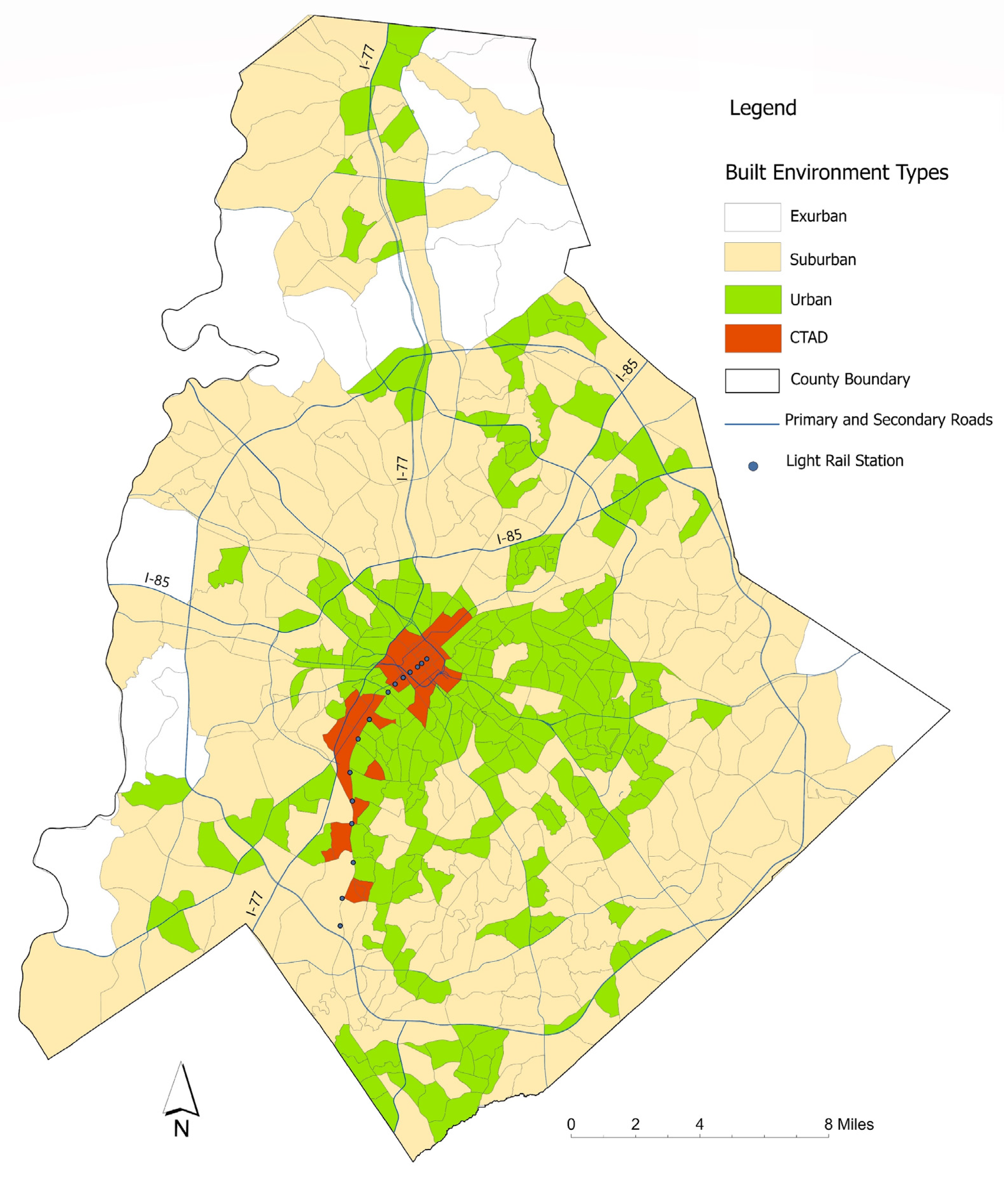
Figure 1 shows the results of the built environment type classification in 2015. Starting from the Bureau of the Census’ definition of urban and rural areas, 16 block groups were identified as exurban, mainly at the periphery of the county. Using the Ward’s clustering method, 252 of the non-rural block groups are classified as suburban, 259 census block groups are identified as urban, mainly in the urban core and along the corridors of development. Finally, 28 census block groups are identified as CTAD. These CTAD areas are located in the CBD and along the south corridor, in proximity to the light rail Blue Line. Statistics of the centroid of each of these clusters are reported in Table 5. The four built-environment types are found to be quite distinct from one another. Comparing the cluster centroids to the county-wide statistics (Table 1) shows that the four built-environment types align well with the sorting of block groups according to their degree of urbanity. As Figure 1 indicates, suburban business districts and edge cities such as the Ballantyne and South Park areas (to the south of the city center), the South End (adjacent to the city center on the southwest side), and the University area (northeast of the city center) are identified as part of the urban area clusters. Some of these clusters, such as the South Park area, provide employment opportunities to the surrounding urban and suburban areas.
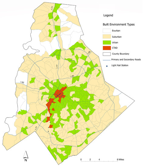
Figure 1.
Classification results for built environment types in Mecklenburg County, NC (2015).
Table 5.
Built environment type cluster centroids (2015).
The coefficients for the (non-spatial) Ordinary Least Squares (OLS) model estimated on a sample of 1092 block groups are reported in Table 6. In this specification, some independent variables were log-transformed to secure homoscedasticity. Based on these results, both CTAD and urban built environment types have a statistically significant impact on commuting duration, all else being equal. Specifically, we find that the average commuting duration in CTAD areas was 1.98 min shorter than in the reference areas (2.576 − 4.554 = −1.978) in 2015. However, for urban areas, their 2015 average commuting duration was longer by 0.36 min (1.084 − 0.726 = 0.358) compared to reference areas. In addition, the average treatment effects show an increase in commuting duration over time in both CTAD and urban built environment types, with coefficients of 2.58 min and 1.08 min, respectively. These two coefficients are equal to the difference in differences between treatment groups and reference groups over time, as shown in Equations (2) and (3). In these equations, y denotes the commuting duration and base denotes the reference group formed of exurban and suburban block groups.
CTAD × year 2015 Coefficient = (yCTAD-2015 − yCTAD-2000) − (ybase-2015 − ybase-2000)
Urban × year 2015 Coefficient = (yUrban-2015 − yUrban-2000) − (ybase-2015 − ybase-2000)
Table 6.
Non-spatial panel data model results.
In contrast, exurban and suburban built environment types have experienced a reduction in commuting duration of 1.52 min from 2000 to 2015. Sociodemographic control variables, including white percentage, African American percentage, Asian percentage, median housing value, median age, Ph.D. degree holders, CBD proximity and car ownership, all have a statistically significant impact on commuting duration, all else being equal.
While the OLS results were an important step in the model building process, we now move on to the analysis with a similarly specified spatial Durbin model, for which estimation results are reported in Table 7. This model was selected among all the spatial models that were tested, including spatial lag, spatial error and spatial error Durbin models, as the best performing model, while avoiding bias and maintaining efficiency. The best model is selected based on the goodness of fit measures of R2, squared correlation coefficient between the fitted values and observed values, maximum likelihood, and after investigating the plots and maps of model residuals. The R2 of the spatial Durbin model is 0.422, which is an improvement of 0.08 over the OLS model.
Table 7.
Spatial Durbin panel data model results.
According to the spatial Durbin model, after controlling for spatial dependence in the dependent variable and in independent variables, CTAD areas have an impact on commuting duration that is significantly different statistically from the suburban and exurban environments, all else being equal. The average commuting duration of CTAD areas was shorter by 0.99 min (2.614 − 3.605 = −0.991) compared to other areas in 2015. Similar to the non-spatial model, commuting duration has increased in both CTAD and urban areas, with average effects of 2.61 min and 0.97 min, respectively, between 2000 and 2015 (Table 7). The coefficient of 2.61 for CTAD areas indicates changes over time in differences in commuting duration between CTAD and reference groups (exurban and suburban). In addition, the coefficient of 0.96 for urban areas shows the differences in commuting duration (minutes) between the urban areas and reference groups (exurban and suburban) and between the two years of 2000 and 2015. Mathematically, the rationale for what these coefficients mean is provided in Equations (1) and (2), respectively. Exurban and suburban areas, on the other hand, experienced a decrease in commuting duration in the order of 1.33 min on average.
Like in the non-spatial model, sociodemographic control variables, including white percentage, African American percentage, Asian percentage, median housing value, median age, Ph.D. degree holders, CBD proximity, and car ownership, have a statistically significant impact on commuting duration, all else being equal. Overall, the spatial Durbin model shows results in line with those of the OLS model.
Mecklenburg County has been experiencing sociodemographic changes (Table 2), mainly as a result of population growth and fast economic development. Accordingly, it has been going through built environment changes such as light rail transit, new compact developments along the planned transit corridors and new employment centers, including Ballantyne, South End, South Park and University areas. As shown in the spatial and nonspatial panel data model results, the changes in commuting duration outcomes over the study period have been affected by the dynamics in sociodemographic and built environment characteristics of Mecklenburg County.
5. Discussion
In order to alleviate the economic, environmental and social consequences of high-cost travel behaviors such as long travel distances or duration, and the consequences of car-dependent travel, new urban planning and design ideas have been advocated, such as new urbanism, sustainable urban development and transit-oriented development. These approaches purport to reduce travel demand and consumption by encouraging density, diversity, design, destination accessibility and reduced distance to transit. There is a considerable body of literature on the relationship between the built environment and travel behavior to evaluate the impact built environment interventions on travel behavior [6,7,8,10,34,56], which stands as a core element of these innovations. These studies have reached diverse conclusions, with some finding statistically significant reduction in travel [11,14,34,35] and others with very slight or no impact [8,28] in neighborhoods with denser and more compact development. One of the shortcomings in this literature is that the majority of studies investigated the relationships in a cross-sectional format while these relationships are fundamentally dynamic. Very few studies have emphasized the longitudinal dimension in this body of literature [23,57].
We pointed out some methodological issues in this body of literature. One of these issues stems from self-selection embedded in the data. Self-selection means that the difference in travel behavior associated with the built environment may have less to do with differences in the built environment itself than with people who in fact self-select themselves into built environments with specific characteristics owing to their travel preferences [23]. Spatial dependence is a second consideration that may distort the true nature of the relationship between the built environment and travel behavior components, including the commuting duration studied here. To alleviate these issues, this study used longitudinal design as a method for removing unobserved factors; the design also controlled for spatial dependence by accounting for the spatial dependence econometrically. By focusing on the difference in differences, we aimed at sorting the impact of the built environment on travel demand.
Spatial panel data model results reveal that both the CTAD and urban built environments have a statistically significant impact on commuting duration, in comparison with our reference groups comprised of exurban and suburban built environments. Both the CTAD and urban areas have shorter commuting duration. However, the average treatment effect increased over the study period in these two areas. In contrast, the exurban and suburban areas experienced a decrease in commuting duration over time. Our analysis results show that the built environment has an impact on commuting duration; however, increase in the 5 Ds of the built environment does not lead to a reduction in commuting duration. Given the importance of such results for policy making in cities that face the thorny challenges of balancing continued growth and land development, on the one hand, and mobility imperatives, on the other, we find our work contributes to understanding the link between travel demand and the built environment. Importantly, we also realize that it does not settle the matter in simple terms, while opening the door to alternative explanations that are broached below.
The apparent lack of consistency between the results of our analysis and large segments of the extant literature begs the question of the possible causes for such differences. In this respect, we believe a highly pertinent observation is that most of the empirical literature treats relatively populous cities, such as Los Angeles, CA, the New York Metropolitan Area, San Diego, CA, Boston, MA, and the San Francisco Bay Area, CA, that are quite mature. Population densities are higher in these case studies than in Charlotte, and transit systems, including subway or light rail systems, have been operating for much longer periods. More transit options are available in these areas, with strong connectivity between different mobility options such as bus and rail. Charlotte stands in sharp contrast as it has an established reputation as a sprawling city [58,59] and has only rather recently experienced a process of densification [60], while the Lynx light rail service is still quite new (it started operation in Fall 2007) and offers low coverage and low connectivity, and has low ridership. These striking differences have several implications on the study of the relationship between the built environment and travel demand. First, by 2015, the residential density of Charlotte’s light rail corridor had increased. This increase may have exacerbated the traffic congestion in those compact areas as the transit system still provided low coverage and low connectivity, which led to an increase in commuting duration of 2.61 min in CTAD and 0.96 min in urban areas. Second, in 2015, the transit and population density may not have been in conditions conducive to encouraging people living in CTAD or urban areas to use transit instead of their personal vehicles. Residents of CTAD areas may still find their personal vehicles more convenient. Thus, these land development and transit network properties may have led to traffic congestion and an increase in commuting duration in compact areas, as policy makers and planners failed to consider their various aspects comprehensively, such as connectivity, coverage, availability of parking facilities near transit stations, and public transit ridership. Along with this point, it can be argued that travel mode is as important as travel duration. As a result, it will be insightful to study commuting duration by travel mode, such as driving to work or using public transit. Third, the suburban and exurban areas of Charlotte have themselves evolved tremendously over the study period, with a frantic pace of land development but also with new highway infrastructure that has succeeded in curbing traffic congestion in these areas.
We contend these differences are critical because, in urban planning and design, compact developments and transit-oriented plans are long-term in nature. Our analysis spans 15 years (2000 to 2015), yet Charlotte is still in search of a “steady state” in its development form and in its transportation infrastructure. For instance, the Charlotte community has recently approved a new transit vision plan [61] that will dramatically enhance the current single-line Lynx service to a fully built-out system, along with integrated land-use planning and transit-oriented development as its cornerstones. As evidence of the evolving mindset and priorities of the community, the City of Charlotte is in the midst of the approval and implementation of a new Comprehensive Plan [62] that espouses the principles of community-centered development with “10-min neighborhoods” as its first goal. Hence, 2015 shows an urban landscape full of nuances that cannot be fully assessed outside of the long-term adjustments towards a new land-use-mobility “equilibrium”. It remains to be seen whether impacts may change in future years, when the transit network properties are improved, and population density is higher. In future conditions of a more populous city, people may have a greater tendency towards using transit.
In addition, the majority of the research on the impact of the built environment on reducing travel consumption has been performed on all trip types, while this work studied work travel. This is important to consider because the response of non-work trips might well be different from work trips in CTAD and urban areas. The 5 Ds may have a greater impact on non-work travel duration or distance than on work travel since the options for services for daily needs and their accessibility increase in compact and diverse neighborhoods.
Given the points raised on the status of residential development, transport infrastructure and mobility in Mecklenburg County in 2015 and given the broader implications this may have on settling the nature of the relationship between the built environment and travel consumption, an agenda can be laid out for future research. First, we propose that cities with diverse degrees of development and transit properties should be studied through comparative approaches to gain insights and shed a better light on the important considerations discussed above.
Second, the longitudinal design method for alleviating the selection bias is based on the assumption that travel preferences are constant over time, while this may not hold true in the fast changing urban context, such as with the emergence of new housing options and new mobility options (e.g., novel Mobility-as-a-Service (MaaS) providers). Having access to primary survey data on travel preferences may help in a better understanding of the role of selection bias for future work.
In addition, given the potential changes in traffic conditions in compact areas during a period of fast transformation of the urban fabric, it would be helpful to control for traffic congestion effects brought about by localized population and employment growth. In addition, with the growing multimodality of urban travel, some measures of walk-and-ride, park-and-ride and other first/last mile coping behaviors should be helpful to the modeling work.
Furthermore, MAUP is another important issue that needs to be considered in studies of the built environment and commuting duration. In this study, the finest level of geography at which the data are available was census block groups. Therefore, possible ecological fallacy cannot practically be circumvented by downscaling the analysis at a finer granularity such as the census blocks. It may be useful, however, to conduct the analysis at the disaggregated level of the individual residents based on travel behavior data.
Lastly, the relationship between the built environment and travel consumption is a multifaceted and multidirectional phenomenon. Bidirectional relationships are possible between different components of travel behavior, such as travel duration, travel distance, travel mode, trip type, trip frequency and mode choice, different factors of the built environment and travel preferences. As a result, more holistic models that can investigate complex relationships in a multidirectional phenomenon, such as structural equation modeling, should be considered for future work.
6. Conclusions
This paper empirically studied the impact of built environment types on commuting duration as a core travel behavior component. There were two hypotheses. First, built environment types have an impact on commuting duration. Second, areas whose urban fabric is deeply associated with density, diversity, design, destination accessibility and reduced distance to transit have shorter commuting duration.
To test the two stated hypotheses, the built environment in 2015 was classified into types of exurban, suburban, urban and CTAD on the basis of built environment factors indicative of the 5 Ds. Their differential impact was then evaluated using spatial panel data models. Spatial econometric results show that the built environment in both CTAD and urban areas has a statistically significant impact on commuting duration in comparison to other built environments, namely the city’s suburbs and exurbs. Both the CTAD and urban areas had shorter commuting durations. However, our analysis reveals that this impact consists of an increase in average treatment effect over time, that is between 2000 and 2015 in our case study, while exurban and suburban areas have experienced a reduction in commuting duration over this period, even after controlling for spatial dependence. It decreased by 1.33 min per commute trip on average in the spatial Durbin model.
In conclusion, the findings of this case study confirm that the built environment is not a neutral context within which travel behavior happens to take place. Statistical evidence tells us that commute duration varies across built-environment types. The results of our case study are similar to others that found a statistically significant impact, although practically small. They are not consistent with the notion that a built environment developed according to the 5 D principles dampens travel demand, however. Instead, they align with studies that have argued that compact developments lead to higher traffic congestion and greater travel duration. We discussed the results of the analysis conducted in the light of the highly dynamic urban environment used for our case study. We argued for the need to direct future research towards enhancing the research design to explicitly accommodate the dynamics of the urban systems where land use structures and the mobility of residents mutually interact.
Author Contributions
Conceptualization, F.H. and J.-C.T.; methodology, F.H. and J.-C.T.; formal analysis, F.H.; investigation, F.H. and J.-C.T.; data curation, F.H.; writing—original draft preparation, F.H.; writing—review and editing, F.H. and J.-C.T.; visualization, F.H.; supervision, J.-C.T.; project administration, J.-C.T. All authors have read and agreed to the published version of the manuscript.
Funding
This research received no external funding.
Institutional Review Board Statement
Not applicable.
Informed Consent Statement
Not applicable.
Data Availability Statement
Not applicable.
Conflicts of Interest
The authors declare no conflict of interest.
References
- Barrington-Leigh, C.; Millard-Ball, A. A century of sprawl in the United States. Proc. Natl. Acad. Sci. USA 2015, 112, 8244–8249. [Google Scholar] [CrossRef] [PubMed]
- US-Department-of-Energy. Annual Vehicle Miles Traveled in the United States. Available online: https://afdc.energy.gov/data/10315 (accessed on 3 February 2022).
- American-Community-Survey. United States Commuting At A Glance: American Community Survey 1-Year Estimates. Available online: https://www.census.gov/topics/employment/commuting/guidance/commuting/acs-1yr.html (accessed on 3 February 2022).
- Jacobs, J. The Death and Life of Great American Cities; Vintage: New York, NY, USA, 1961. [Google Scholar]
- Crane, R. The Influence of Urban Form on Travel: An Interpretive Review. J. Plan. Lit. 2000, 15, 3–23. [Google Scholar] [CrossRef]
- Ewing, R.; Cervero, R. Travel and the Built Environment: A Synthesis. Transp. Res. Rec. J. Transp. Res. Board 2001, 1780, 87–114. [Google Scholar] [CrossRef]
- Ewing, R.; Cervero, R. Travel and the Built Environment: A Meta-Analysis. J. Am. Plan. Assoc. 2010, 76, 265–294. [Google Scholar] [CrossRef]
- Stevens, M.R. Does Compact Development Make People Drive Less? J. Am. Plan. Assoc. 2017, 83, 7–18. [Google Scholar] [CrossRef]
- Cao, X.; Mokhtarian, P.L.; Handy, S.L. Do changes in neighborhood characteristics lead to changes in travel behavior? A structural equations modeling approach. Transportation 2007, 34, 535–556. [Google Scholar] [CrossRef]
- Cervero, R.; Murakami, J. Effects of Built Environments on Vehicle Miles Traveled: Evidence from 370 US Urbanized Areas. Environ. Plan. A Econ. Space 2010, 42, 400–418. [Google Scholar] [CrossRef]
- Chen, C.; Gong, H.; Paaswell, R. Role of the built environment on mode choice decisions: Additional evidence on the impact of density. Transportation 2008, 35, 285–299. [Google Scholar] [CrossRef]
- Izanloo, A.; Rafsanjani, A.K.; Ebrahimi, S.P. Effect of Commercial Land Use and Accessibility Factor on Traffic Flow in Bojnourd. J. Urban Plan. Dev. 2017, 143, 05016016. [Google Scholar] [CrossRef]
- Khattak, A.J.; Rodriguez, D. Travel behavior in neo-traditional neighborhood developments: A case study in USA. Transp. Res. Part A Policy Pract. 2005, 39, 481–500. [Google Scholar] [CrossRef]
- Salon, D. Heterogeneity in the relationship between the built environment and driving: Focus on neighborhood type and travel purpose. Res. Transp. Econ. 2015, 52, 34–45. [Google Scholar] [CrossRef]
- Zhou, B.B.; Kockelman, K.M. Self-Selection in Home Choice: Use of Treatment Effects in Evaluating Relationship Between Built Environment and Travel Behavior. Transp. Res. Rec. J. Transp. Res. Board 2008, 2077, 54–61. [Google Scholar] [CrossRef]
- Bagley, M.N.; Mokhtarian, P.L. The impact of residential neighborhood type on travel behavior: A structural equations modeling approach. Ann. Reg. Sci. 2002, 36, 279–297. [Google Scholar] [CrossRef]
- Crane, R.; Crepeau, R. Does neighborhood design influence travel?: A behavioral analysis of travel diary and GIS data. Transp. Res. Part D Transp. Environ. 1998, 3, 225–238. [Google Scholar] [CrossRef]
- Etminani-Ghasrodashti, R.; Ardeshiri, M. Modeling travel behavior by the structural relationships between lifestyle, built environment and non-working trips. Transp. Res. Part A Policy Pract. 2015, 78, 506–518. [Google Scholar] [CrossRef]
- Nasri, A.; Zhang, L. Assessing the Impact of Metropolitan-Level, County-Level, and Local-Level Built Environment on Travel Behavior: Evidence from 19 U.S. Urban Areas. J. Urban Plan. Dev. 2015, 141, 04014031. [Google Scholar] [CrossRef]
- Wang, K. Causality between Built Environment and Travel Behavior: Structural Equations Model Applied to Southern California. Transp. Res. Rec. J. Transp. Res. Board 2013, 2397, 80–88. [Google Scholar] [CrossRef]
- Boarnet, M.; Crane, R. The influence of land use on travel behavior: Specification and estimation strategies. Transp. Res. Part A Policy Pract. 2001, 35, 823–845. [Google Scholar] [CrossRef]
- Cao, X.J.; Xu, Z.; Fan, Y. Exploring the connections among residential location, self-selection, and driving: Propensity score matching with multiple treatments. Transp. Res. Part A Policy Pract. 2010, 44, 797–805. [Google Scholar] [CrossRef]
- Mokhtarian, P.L.; Cao, X. Examining the impacts of residential self-selection on travel behavior: A focus on methodologies. Transp. Res. Part B Methodol. 2008, 42, 204–228. [Google Scholar] [CrossRef]
- Ghose, A. Problems of endogeneity in social science research. In Research Methodology for Social Sciences, 1st ed.; Acharyya, R., Bhattacharya, N., Eds.; Routledge: London, UK, 2019; pp. 218–252. [Google Scholar]
- Cliff, A.D.; Ord, K. Spatial Autocorrelation: A Review of Existing and New Measures with Applications. Econ. Geogr. 1970, 46, 269. [Google Scholar] [CrossRef]
- Thill, J.-C. Research on Urban and Regional Systems: Contributions from GIS&T, Spatial Analysis, and Location Modeling. In Innovations in Urban and Regional Systems; Thill, J.-C., Ed.; Springer International Publishing: Cham, Switzerland, 2020; pp. 3–20. [Google Scholar]
- Fotheringham, A.S.; Wong, D.W. The modifiable areal unit problem in multivariate statistical analysis. Environ. Plan. A 1991, 23, 1025–1044. [Google Scholar] [CrossRef]
- Cervero, R.; Kockelman, K. Travel demand and the 3Ds: Density, diversity, and design. Transp. Res. Part D Transp. Environ. 1997, 2, 199–219. [Google Scholar] [CrossRef]
- Handy, S. Regional Versus Local Accessibility: Implications for Nonwork Travel; UC Berkeley, University of California Transportation Center: Berkeley, CA, USA, 1993; Volume 18, pp. 253–267. Available online: https://escholarship.org/uc/item/2z79q67d (accessed on 11 April 2022).
- Ewing, R.; Tian, G.; Goates, J.; Zhang, M.; Greenwald, M.J.; Joyce, A.; Kircher, J.; Greene, W. Varying influences of the built environment on household travel in 15 diverse regions of the United States. Urban Stud. 2015, 52, 2330–2348. [Google Scholar] [CrossRef]
- Handy, S.; Cao, X.; Mokhtarian, P.L. Self-Selection in the Relationship between the Built Environment and Walking: Empirical Evidence from Northern California. J. Am. Plan. Assoc. 2006, 72, 55–74. [Google Scholar] [CrossRef]
- Nasri, A.; Zhang, L. Impact of Metropolitan-Level Built Environment on Travel Behavior. Transp. Res. Rec. J. Transp. Res. Board 2012, 2323, 75–79. [Google Scholar] [CrossRef]
- Handy, S.; Cao, X.; Mokhtarian, P. Correlation or causality between the built environment and travel behavior? Evidence from Northern California. Transp. Res. Part D Transp. Environ. 2005, 10, 427–444. [Google Scholar] [CrossRef]
- Cervero, R. Built environments and mode choice: Toward a normative framework. Transp. Res. Part D Transp. Environ. 2002, 7, 265–284. [Google Scholar] [CrossRef]
- Cervero, R.; Duncan, M. ’Which Reduces Vehicle Travel More: Jobs-Housing Balance or Retail-Housing Mixing? J. Am. Plan. Assoc. 2006, 72, 475–490. [Google Scholar] [CrossRef]
- Zhang, L.; Nasri, A.; Hong, J.H.; Shen, Q. How built environment affects travel behavior: A comparative analysis of the connections between land use and vehicle miles traveled in US cities. J. Transp. Land Use 2012, 5, 40–52. [Google Scholar] [CrossRef]
- Leck, E. The Impact of Urban Form on Travel Behavior: A Meta-Analysis. Berkeley Plan. J. 2011, 19, 37–58. [Google Scholar] [CrossRef]
- Guerra, E. The Built Environment and Car Use in Mexico City: Is the Relationship Changing over Time? J. Plan. Educ. Res. 2014, 34, 394–408. [Google Scholar] [CrossRef]
- Jin, Y.; Denman, S.; Deng, D.; Rong, X.; Ma, M.; Wan, L.; Mao, Q.; Zhao, L.; Long, Y. Environmental impacts of transformative land use and transport developments in the Greater Beijing Region: Insights from a new dynamic spatial equilibrium model. Transp. Res. Part D Transp. Environ. 2017, 52, 548–561. [Google Scholar] [CrossRef]
- Ward, J.H. Hierarchical Grouping to Optimize an Objective Function. J. Am. Stat. Assoc. 1963, 58, 236–244. [Google Scholar] [CrossRef]
- Manville, M. Travel and the Built Environment: Time for Change. J. Am. Plan. Assoc. 2017, 83, 29–32. [Google Scholar] [CrossRef]
- Sun, B.; Yin, C. Impacts of a multi-scale built environment and its corresponding moderating effects on commute duration in China. Urban Stud. 2020, 57, 2115–2130. [Google Scholar] [CrossRef]
- Sun, B.; Ermagun, A.; Dan, B. Built environmental impacts on commuting mode choice and distance: Evidence from Shanghai. Transp. Res. Part D: Transp. Environ. 2017, 52, 441–453. [Google Scholar] [CrossRef]
- Zhu, P.; Ho, S.N.; Jiang, Y.; Tan, X. Built environment, commuting behaviour and job accessibility in a rail-based dense urban context. Transp. Res. Part D Transp. Environ. 2020, 87, 102438. [Google Scholar] [CrossRef]
- Zhu, P.; Zhao, S.; Jiang, Y. Residential segregation, built environment and commuting outcomes: Experience from contemporary China. Transp. Policy 2022, 116, 269–277. [Google Scholar] [CrossRef]
- LaCour, G. Light-Rail Tab Unveiled. Available online: https://en-academic.com/dic.nsf/enwiki/4679322 (accessed on 25 May 2022).
- City of Charlotte. 2030 Transit Corridor System Plan. Available online: https://charlottenc.gov/cats/transit-planning/2030-plan/Pages/default.aspx (accessed on 3 June 2021).
- Manson, S.M. IPUMS National Historical Geographic Information System: Version 15.0. 2020. Available online: https://data2.nhgis.org/main (accessed on 5 May 2021).
- Mecklenburg-County-GIS-Center. 2017. Available online: https://www.mecknc.gov/LUESA/GIS/Pages/GIS-Data-Center.aspx (accessed on 1 August 2020).
- United States Census Bureau. LEHD Origin-Destination Employment Statistics Data. 2017. Available online: https://lehd.ces.census.gov/data/ (accessed on 20 May 2020).
- United States Census Bureau. 2010 Census Urban and Rural Classification and Urban Area Criteria. 2010. Available online: https://www.census.gov/programs-surveys/geography/guidance/geo-areas/urban-rural/2010-urban-rural.html (accessed on 20 May 2020).
- Song, Y.; Merlin, L.; Rodriguez, D. Comparing measures of urban land use mix. Comput. Environ. Urban Syst. 2013, 42, 1–13. [Google Scholar] [CrossRef]
- Anselin, L. Local Indicators of Spatial Association-LISA. Geogr. Anal. 1995, 27, 93–115. [Google Scholar] [CrossRef]
- Anselin, L.; Bera, A. Spatial dependence in linear regression models with an introduction to spatial econometrics. In Handbook of Applied Economic Statistics; CRC Press: Boca Raton, FL, USA, 1998; pp. 237–289. Available online: http://www.econ.uiuc.edu/~hrtdmrt2/Teaching/SE_2016_19/References/Spatial_Dependence_in_Linear_Regression_Models_With_an_Introduction_to_Spatial_Econometrics_281_29.pdf (accessed on 11 April 2022).
- Elhorst, J.P. Matlab Software for Spatial Panels. Int. Reg. Sci. Rev. 2014, 37, 389–405. [Google Scholar] [CrossRef]
- Cao, X.J.; Mokhtarian, P.L.; Handy, S.L. The relationship between the built environment and nonwork travel: A case study of Northern California. Transp. Res. Part A Policy Pract. 2009, 43, 548–559. [Google Scholar] [CrossRef]
- Wang, D.; Lin, T. Built environment, travel behavior, and residential self-selection: A study based on panel data from Beijing, China. Transportation 2019, 46, 51–74. [Google Scholar] [CrossRef]
- Song, Y.; Knaap, G.-J. Measuring Urban Form: Is Portland Winning the War on Sprawl? J. Am. Plan. Assoc. 2004, 70, 210–225. [Google Scholar] [CrossRef]
- Wilson, B.; Song, Y. Comparing apples with apples: How different are recent residential development patterns in Portland and Charlotte? J. Urban. Int. Res. Placemaking Urban Sustain. 2009, 2, 51–74. [Google Scholar] [CrossRef]
- Delmelle, E.; Zhou, Y.; Thill, J.-C. Densification without Growth Management? Evidence from Local Land Development and Housing Trends in Charlotte, North Carolina, USA. Sustainability 2014, 6, 3975–3990. [Google Scholar] [CrossRef]
- Charlotte-Area-Transit-System. 2030 Transit System Corridor Plan. Available online: https://charlottenc.gov/cats/transit-planning/2030-plan/Documents/2030_Transit_Corridor_System_Plan.pdf (accessed on 10 October 2020).
- City-of-Charlotte. Charlotte Future 2040 Comprehensive Plan. Available online: https://www.cltfuture2040plan.com/sites/all/themes/custom/smoky_hollow/docs/CF2040_Public-Review-Draft-Plan_Web.pdf (accessed on 25 May 2022).
Publisher’s Note: MDPI stays neutral with regard to jurisdictional claims in published maps and institutional affiliations. |
© 2022 by the authors. Licensee MDPI, Basel, Switzerland. This article is an open access article distributed under the terms and conditions of the Creative Commons Attribution (CC BY) license (https://creativecommons.org/licenses/by/4.0/).