The Role of Learning in Adaptation to Technology: The Case of Groundwater Extraction

Abstract

Learning may play an important role in adopting new technology. While the role of learning in the decision to adopt has been widely investigated in the literature, to the best of our knowledge its role in knowing how to best use technology and the speed of learning has not been studied extensively. An example of this situation is when farmers adopt groundwater extraction technology. In this case, they need to learn the exact cost and benefit of extracting water in is relation to how they use it in practice. By comparing the extraction behavior of farmers who own new wells with farmers who own old wells, this paper explores the role of experience in shaping farmers’ decisions. Three identification strategies are used in this study to test the hypothesis that owners with less experience (owners of new wells) with groundwater technology are able to extract more water than experienced owners. The first strategy employs panel data. The results of this model show that groundwater extraction rises as the growth rate in the number of new wells increases. The second strategy uses the exogenous variation in precipitation shocks in a double-difference approach. Employing census data at the well level, this study shows that 6–13% more water is extracted from new wells than from older wells, and that the difference in extraction increases in areas that experience negative precipitation shocks. The third strategy uses the nearest-neighbor matching method, which shows that new wells extract 11% more groundwater per year compared to old wells, indicating that old wells are more efficient in maintaining their inter-temporal extraction. These findings have important implications for discussions of regulating a common pool resource. In the literature regarding the common pool problem, firms are often considered entities with complete information about their true abatement costs. An implication of findings of this paper is that quantity instruments for regulating groundwater extraction fail to guarantee productive efficiency when farmers face uncertainty about their marginal abatement cost. The results of this study show that it takes a few years for farmers to adapt to new technologies. According to this finding, a recommendation to policy makers, therefore, is that they must consider this time lag in learning how to use new technologies when proposing policies to mitigate the effects of climate change.

1. Introduction

Groundwater is a natural resource that is subject to the common pool problem. Achieving optimal extraction for a common pool resource requires market or non-market tools that are either imposed by a government or agreed upon through coordination of private stakeholders [1,2]. Price interventions, taxes, and quotas are more popular examples of tools for government intervention, each having benefits that depend on the nature of the problem and the objective of the regulator [3,4,5,6,7,8]. There are less popular methods as well, such as public provision. For example, Sekhri [9] shows that public provision reduced over-extraction in rural India, where the fixed cost of extraction is high.

A conventional assumption in modeling government regulation of a common pool is that while the regulator does not know the true abatement cost (the cost of reducing usage), the firm has complete information about its cost structure, including the abatement cost [10,11,12,13,14,15]. This assumption may not hold in certain practical cases, at least in the short run, i.e., even firms may have incomplete information about their costs. This scenario involving an incomplete information problem is more likely to exist when a new technology is adopted by a firm, for the following two reasons: The firm has to learn the true costs and benefits of using the new technology, and part of this information might be firm- or technology-specific, meaning that it must be learned by acquiring experience with the new technology [16]. Second, even if the firm knows the abatement cost of the new technology, it may not possess the knowledge to use the new technology efficiently [17]. For these reasons, it may take time for firms to learn their exact costs with respect to using a new technology.

The new technology that is studied in this paper is the pumping of groundwater by farmers. When farmers use groundwater in production activities for the first time as a new technology they know the nominal characteristics of this technology, such as the information on the label of the pump with regard to energy usage. In practice, however, the actual energy consumption depends on many factors that differ from one well to another, such as the depth to water and the characteristics of the soil [18]. These well-specific factors affect the actual amount of energy consumption per unit of water extracted. In addition, farmers must learn how to manage their inter-temporal extraction in order to maintain their production from planting to harvest [19].

The effects of experience in working with new technology are investigated in this study. Our main focus is to show that in their early years using groundwater extraction, farmers do not use it in the same manner as those with more experience with the same technology. Moreover, this paper explores whether this difference in extraction by farmers has any implications in terms of their ability to maintain their water resources throughout the planting to harvesting period.

This study benefits from a novel dataset, Iran’s Census of Wells, which provides information on about 730,000 wells in all provinces of the country. To the best of our knowledge, this is the first study that uses a census of all wells in a country to study adaptation to technology. The geographical dispersion of the wells over regions with different climates considerably reduces the external validity concerns that are inherent in studies focused on smaller regions.

2. Literature Review

One of the challenges for sustainable development in the climate change era is to find strategies to cope with the increased variability in weather parameters such as precipitation and temperature. Agriculture is one of the sectors that suffers most from variable precipitation and temperature [20]. Technology plays an important role in the ability of agrarians to adapt to the changing climate. New technologies in the form of resistant crops, irrigation and plantation methods, and the use of groundwater can enable farmers to maintain production when local temperature and precipitation patterns change [7]. There is often a significant interval between the time that a new technology is first developed and available in the market and the time that it becomes widely used by producers [21]. However, diffusion of new technologies depends on factors such as knowledge and availability of information about the new technology [22,23,24], perception of farmers about the performance of new technology [25], schooling, access to credit, contact with extension agents [26], farmers’ networks [27], and even the gender of farmers [28]. Even after adopting new technology, farmers need to learn how to employ it in practice. Studies on learning from this point of view are scant in the literature. Foster and Rosenzweig [29], for example, show that as farmers’ experience with a new technology increases, their profit increases as well, which implies that learning continues after a new technology is adopted.

Farmers find out about the true costs and benefits of using a new technology through learning by doing. A related notion of learning by doing, or learning by experience, has been the subject of a strand of literature in the theory of consumer choice studying experience goods [30,31,32,33]. An experience good is defined as a new product for which consumers do not have perfect knowledge of the true costs and benefits of using it. In this case, consumers learn about different characteristics of the experience good, such as quality, as they use it over time [34]. This view of learning is close to the scope of the current study. Farmers who adopt a new technology, such as groundwater extraction, need to learn about such important features as the short-term and long-term costs of production, the seasonal pattern of depth to groundwater, velocity of water and other hydrological variables, how to maintain their crops, pump characteristics, etc., concerning the new technology.

This paper adds to the above literature by claiming that the true costs of using groundwater, in terms of the ability to maintain extraction even in the short term, are typically not known to a farmer who has recently adopted the new technology of groundwater use. For example, farmers with experience using groundwater employ practices that allow them to have smaller seasonal variations in water extraction compared to those with less experience. A study close to this view has been conducted by Hintermann and Lange [35], who used the experience good framework to show how taxes and/or subsidies can be used to help consumers learn the true costs of replacing a more polluting technology. The main objective of Hinterman and Lange [35] is to develop a mechanism to increase the adoption of new technology. By contrast, the goal of this article is to show that learning can make farmers more efficient in the use of an already-adopted technology.

3. Materials and Methods

3.1. Data

Five sources of data are employed in this article. The first set of data consists of panel data constructed from two consecutive agricultural censuses taken eleven years apart, in 2003 and 2014. The next set of data is a census of all wells in Iran, which was carried out between 2003 and 2013. Piezometric data are used to estimate the change in the groundwater level and obtain a time series of groundwater extraction, which is then matched with the panel data. The last data source consists of precipitation and temperature data from local weather stations in Iran. In the following subsections, the different data sources used in this manuscript are discussed in greater detail.

3.1.1. Panel Data

The first set of data in this study is a panel constructed from the agricultural census collected by [36]. The agricultural census is a country-wide census that includes both agricultural activities and information from villages on their water resources, availability of agricultural machinery and related services, and livestock. As for any other kind of census, agricultural censuses are costly, and are normally conducted about every ten years in Iran. The Statistical Center of Iran (SCI) conducted this census in 1971, 1988, 1993, 2003, and 2014. Although the SCI collected census data almost every decade, for consistency of variables and availability reasons this article only uses the most recent two rounds.

Most of the collected variables are reported at the district level; thus, district was set as the cross-section dimension of the panel. The census is based on the official administrative divisions in each particular year. During the ten year period between rounds of the census, an additional province was created (Iran had 30 provinces in 2003 and 31 provinces in 2014) along with 113 more districts (districts increased from 315 to 428). All new divisions were merged with their previous components and computed all variables for the resulting balanced panel. In the regression analysis, only 298 districts were used due to a lack of other variables (mainly groundwater extraction data, as explained in Section 3.1.3 below).

Table 1. Summary statistics of the agricultural censuses of 2003 and 2014.

	2003		2014
Variable	Mean	Standard	Mean	Standard
		Deviation		Deviation
Total land under ag/district area	0.19	0.14	0.17	0.14
Total planted/total land under ag	0.72	0.18	0.77	0.17
Gardening/Farming	1.3	12.1	2.02	26.34
Total irrigated/total land under ag	0.58	0.31	0.59	0.32
Wheat/total farming	0.36	0.2	0.36	0.21
Irrigated wheat/total wheat	0.48	0.36	0.46	0.37
Rural pop/total	0.47	0.2	0.41	0.19
Growth in # of wells	21.73	79.64	22.23	81.59
# of wells per km2	0.65	1.04	1.21	1.95
Positive precipitation shock	0.23	0.42	0.02	0.14
Negative precipitation shock	0.03	0.18	0.17	0.37
# of positive precipitation shock in past 3 years	0.05	0.23	0.2	0.46
# of negative precipitation shock in past 3 years	0.7	0.71	0.44	0.62
Extraction per well (thousand m3)	130.12	125.71	89.97	95.97
Total extraction per irrigated land (thousand m3/km2)	641,717	869,598	716,716	917,644
Observations	315		315

Source: Statistical Center of Iran (SCI), Agricultural census (2003–2014).

summarizes the main variables in the regression analysis. As can be seen from the table, in 2014 more districts experienced a negative shock and fewer districts experienced a positive shock. Two variables were defined to summarize past positive or negative shocks. The number of positive (negative) precipitation shocks in the past three years counts the number of positive (negative) shocks for those districts that did not experience negative (positive) shocks in the same time frame. The number of shocks is defined based on the three past years, and thus does not overlap with the positive (negative) precipitation shock indicator.

As can be seen in Table 1, in 2014, a smaller share of land was assigned to agricultural activities, while a greater share of the assigned land was actually under cultivation. Moreover, from 2003 to 2014 more land was assigned to gardening, and slightly more land was irrigated as opposed to rain-fed. While the area under wheat production stayed the same, a higher percentage of wheatland was rain-fed in 2014. The share of the rural population decreased, and both the number of wells and the density of wells per km² increased between 2003 and 2014. Because total extraction stayed almost fixed, extraction per well decreased and extraction per irrigated hectare increased.

In order to provide more context for agriculture in Iran, the cultivated area has remained fairly constant over a long period based on the agricultural census. The total planted area of the country declined from 13,073 thousand Hectares (Ha) to 12,744 thousand Ha between the 2003 and 2014 rounds of the Iranian Agricultural Census. The irrigated area in the same period has risen from 6360 thousand Ha to 6426 thousand Ha. While both of these measures show almost no change, they do show a slight substitution towards more irrigation. In the 2003–2014 period, agricultural output grew at a rate of 1.74 percent per year on average.

3.1.2. Wells Census

The second source of data is the census of wells collected by [37], which provides information about all wells in the country. The Iran Water Resource Management Company (IWRMC) began collecting these data 2003, initially surveying two to five provinces each year and collecting information about all wells in those provinces and then moving on to other provinces. Thus, the census is spread over the years 2003 to 2013. Because the data for wells located near the borders of the country are not publicly available and the released data only cover the years up to 2013, the total number of wells in the dataset is 729,220, of which 526,917 (72.26%) are operational. The rest are either being drilled (0.3%), not equipped (5.15%), have a technical problem in the well structure (0.32%), a technical problem with equipment (1.1%), were shut down at the time of the visit (4.84%), temporarily shutdown (4.48%), had no water (4.76%), were abandoned (4.67%), or had another non-working status (2.13%).

The main use of the extracted water is for agriculture purposes, which is defined as either farming (84.95%), greenhouse planting (0.27%), or growing herbs (0.08%). The rest of the wells are used for drinking water (5.20%), livestock, fisheries, landscaping (4.73%), in industry (2.58%), and in the service sector (2.19%). Because the objective is to model extraction behavior in the agricultural sector, our analysis here covers only those wells that are used at least partially for agricultural activities (farming, greenhouses, and herb production) and have a non-missing extraction value. Considering only this group of wells, the number of wells in the sample is 407,824. The age of wells is another important variable, and was not computable for 6908 wells as either the survey year or establishment year for the well was missing. Finally, a number of wells were lacking other explanatory variables included in the regression analysis (mostly the well depth). Thus, most of the regressions in this paper that use the census of wells rely on a final number of 395,306 observations.

Table 2. Summary statistics from Wells Census (2003–2013).

Variable	Mean	Std. Dev.	Min.	Max.
Depth	40.72	44.67	4	450
Water tank	0.18	0.39	0	1
Elevation	914	737	−28.68	3179
Slope	0.89	1.3	0	25.70
Distance to the nearest city (km)	8.56	9.83	0	99.85
Number of wells in 10 km radius	96	115	0	1582
Age of well	15.72	10.67	0	107
Flow of water	8.64	9.63	0.01	102.4
Newly established well	0.04	0.2	0	1
Positive precipitation shock	0.13	0.34	0	1
Negative precipitation shock	0.27	0.44	0	1
Positive precipitation shocks in past three years	0.18	0.40	0	2
Negative precipitation shocks in past three years	0.45	0.53	0	2
Extraction (m3)	88,036	172,633	0	2,838,240
Extraction for ag. purposes (m3)	87,061	171,473	0	2,838,240
Irrigation method
Flooding	0.89
Furrow	0.05
Pressurized	0.06
Number of seasons worked
one	0.04
two	0.31
three	0.33
four	0.32
Observations	400,916

Source: Iran Water Resource Management Company (2003–2013).

summarizes the main variables used in the regression analysis in Section 4.2. Here, we provide a brief explanation of the most important statistics. The slope variable shows that most of the wells are in flat areas. This is consistent with the fact that most of the wells in Iran are used for flooding irrigation systems. Very few wells are in urban areas; the majority are in rural areas or on farms located outside of towns. Areas of the country are heterogeneous in terms of their well density; in certain areas wells have more than 1500 other wells within a 10 km radius, while in other areas there are far fewer. Although we provide an extensive discussion of precipitation shocks, it is obvious at a glance that many of the wells experienced a negative precipitation shock in both the survey year and in the three years prior to the interview date. Moreover, very few farmers use wells for irrigation in only one season of the year.

One variable that is important to mention here is “extraction for agriculture purposes”. As mentioned above, extracted water has different usages, and the modeling here only includes the part that is used for agriculture. There are cases where the well has mixed usage. For example, a person might own a well that is used for drinking in a rural area and use the remaining water for farming or a greenhouse, or a well could be used for a combination of industry, service, and farming. Fortunately, for almost all wells the percentage of water that is devoted to each activity is specified. In the regressions, both total extraction and “extraction for agriculture purposes”, which is the share of the total extraction used for agricultural activities, are employed.

Finally it is worth mentioning that the distinction between ownership of a new well and experience is important for the purposes of this study. Owners of new wells in the agriculture sector in Iran possess limited, if any, experience in working with groundwater technology. The majority of farmers in Iran operate a small amount of land (see [38,39]). As can be seen in Figure 1, 37% of farms have an area of less than 1 ha, and 38% have an area of between 1 and 5 ha. Moreover, while there are more than four million farming units, there are only five hundred thousand wells in the country. Therefore, it is expected that most of the owners of wells in the agriculture sector use at most one well.

There is a great deal that owners of new wells must learn by doing, even if they have operated a well before. There is much local and even well-specific information that a farmer needs to learn. Two wells that are close to each other may have different depths, purposes, pumps, structures, etc. Therefore, the optimal (private) extraction level of one well may not be optimal for its neighbor. Even if the two wells were similar in all aspects, their owners may not trust the information they receive from more experienced neighbors [29]. As a result, farmers may even systematically ignore information that might help them to adapt to the new technology. The latter two points indicate that, while there is a lot for owners of new wells to learn, even when information is available to them publicly or through networks they must acquire at least part of it through experience and learning by doing.

3.1.3. Piezometric Data and Aggregate-Level Water Consumption

Water extraction depends on the availability of water under the ground. The IWRMC manages and reports piezometric data, and has recorded these data from 1964 to the present. Piezometric data are collected from piezometers, which are tubes “placed in the soil to depths below the water table and that extends to the soil surface” [40]. Piezomters are used to measure the “elevation of the free water table [ … ] relative to the soil surface” [40]. More recently, these data have been gathered for more than 13,000 wells in order to monitor groundwater levels. As mentioned in Section 3.1.2, the IWRMC does not report any data (neither well records nor piezometric data) in areas close to the borders of the country. That is why there are only have 12,912 piezometric wells available in the data, all of them marked as non-border, in the data from the IWRMC.

The monitoring system needs to be explained. The IWRMC divides the country into six major water basins, 30 smaller aquifers (second degree), 367 zones, and 11,138 localities. As one can imagine, each locality is a small area. The data are available for multiple wells for each locality, and 90% of the time the depth to water (distance from the land surface to the water in the well when not pumping) in the specific piezometric well is measurable, i.e., the well is functional. There are multiple reasons why a piezometric well might not work. The most important reason is that the well dries out (40%). Whenever a well does not work, the IWRMC digs another well in the same locality. In this paper, each well from the census data was connected to the nearest piezometric well which has at least four consecutive years of data. More than half of the wells in the census were able to be connected to a piezometric well less than 30 km away.

Another source of data provided by IWRMC is the total amount of water extraction and consumption from underground and surface water. These data are collected using a sample of wells and natural springs in each area, information from all dams and rivers, and from precipitation and evaporation estimates. Researchers have extensively studied the relationship between precipitation and groundwater [41,42], the recharge rate of groundwater [43,44,45], and groundwater flow [46]. In a nutshell, a water accounting framework is usually used with the help of hydrological equations to compute the change in the reservoir of water available in each area. Precipitation, surface and underground flows entering the reservoir, and water transferred to the area are the sources of water used in water accounting, while evaporation, outgoing flows from surface and groundwater, and water transferred out of the area are the main ways in which water leaves an area. The IWRMC uses the same approach to estimate groundwater consumption, considering groundwater flow to the area, precipitation, incoming flows from surface waters, irrigation, drinking water waste from rural and urban areas, water waste from the industrial sector, outgoing flows of the groundwater from the area, evaporation, and extraction from wells, qanats, and natural springs [47,48].

We computed the amount of extracted groundwater for each district based on the reported extraction for different zones. When the boundaries of zones defined by the IWRMC did not coincide with the boundaries of districts defined by the SCI, the extraction for a zone was distributed between two neighboring districts based on their respective share of the zones’ combined area. Another important modification was to drop certain districts, as the IWRMC does not report extraction for areas close to the borders of the country.

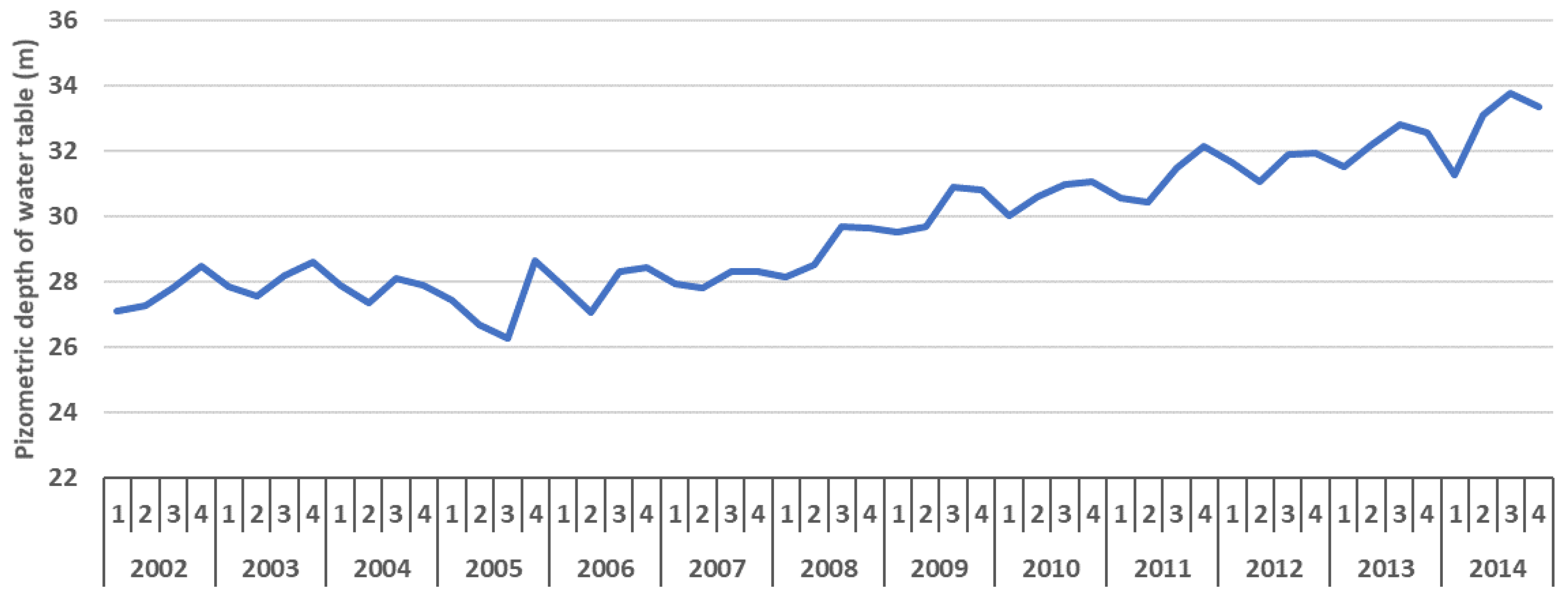
The dependency of agriculture on groundwater together with higher demand for it due to the growing population has resulted in the depletion of groundwater resources. Figure 2 shows the average depth to water for the whole country. The depth to water has steadily increased throughout the 2002–2014 period, and the rate of depletion increases after 2008. From 2002–2014 the depth to water increased from 27.6 m to 33.6 m, with a yearly average increase of 1.7 percent.

3.1.4. Weather Data

This study used station-based precipitation and temperature data. The available data begin in 1952 with 17 weather stations for precipitation and temperature. Currently, the Iran Meteorological Organization (IRIMO) publishes weather data from 362 stations on an hourly basis; monthly precipitation and temperature data are available with a short lag. In order to obtain a consistent long-term mean of precipitation for the panel data models, the average precipitation and temperature in a district was determined only from stations for which there was continuous data between 1990 and 2014. After computing the precipitation, the positive and negative shocks for each district were defined. In a particular year, the negative shock indicator takes a value of one when the rainfall is more than one standard deviation below the average rainfall in the 1990–2014 period. Similarly, if the rainfall is higher than one standard deviation above the mean, the variable for positive precipitation shock takes a value of one.

In order to study the effects of precipitation shocks on the behavior of extraction from wells (well-level data), each well was connected to the closest weather station and the precipitation and temperature data from that station were used for estimations. Again, only stations which continuously reported data between 1990 and 2014 were used. Table 1 and Table 2 show the percentage of districts and wells that experienced a positive shock and the percentage that experienced a negative shock.

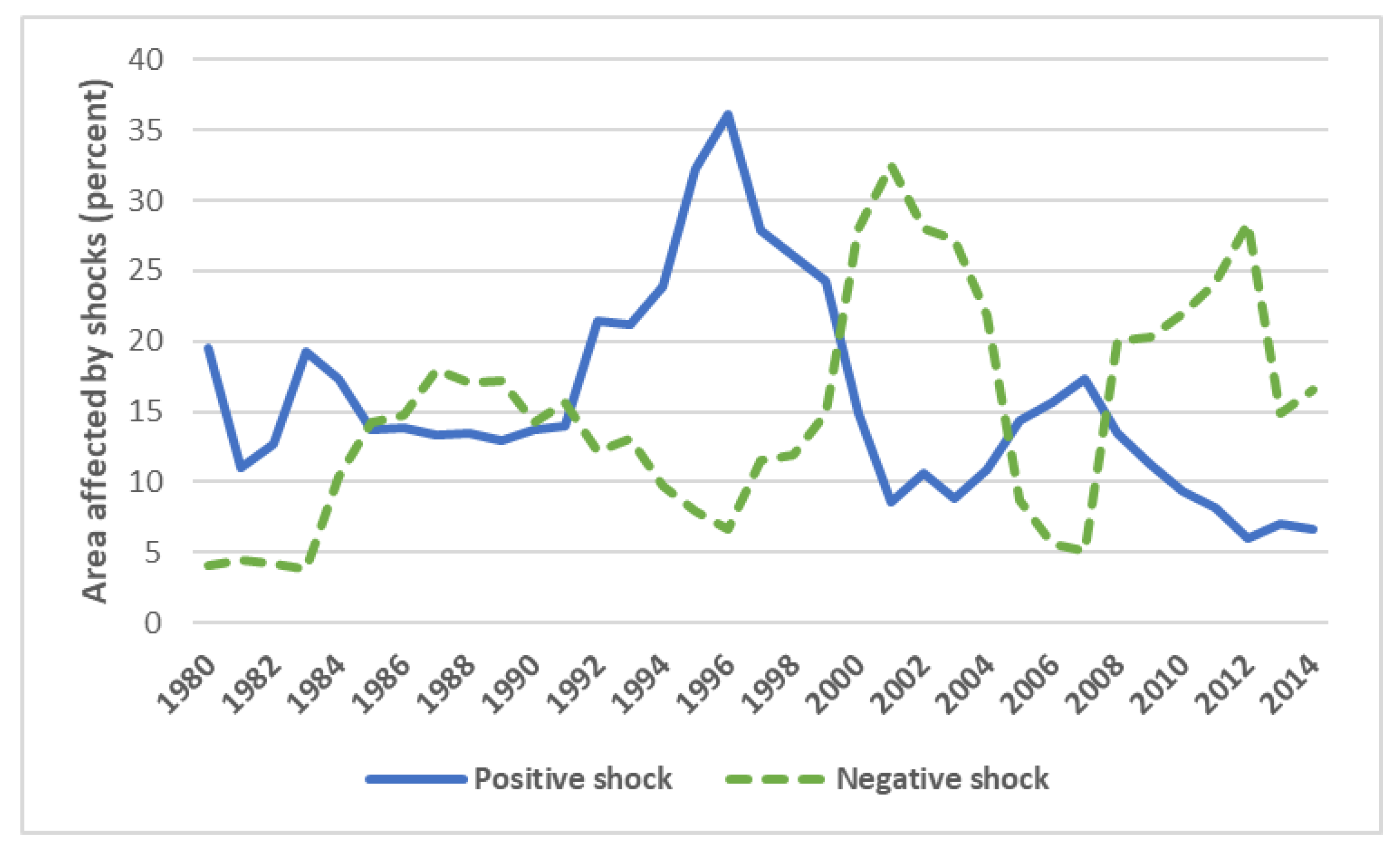
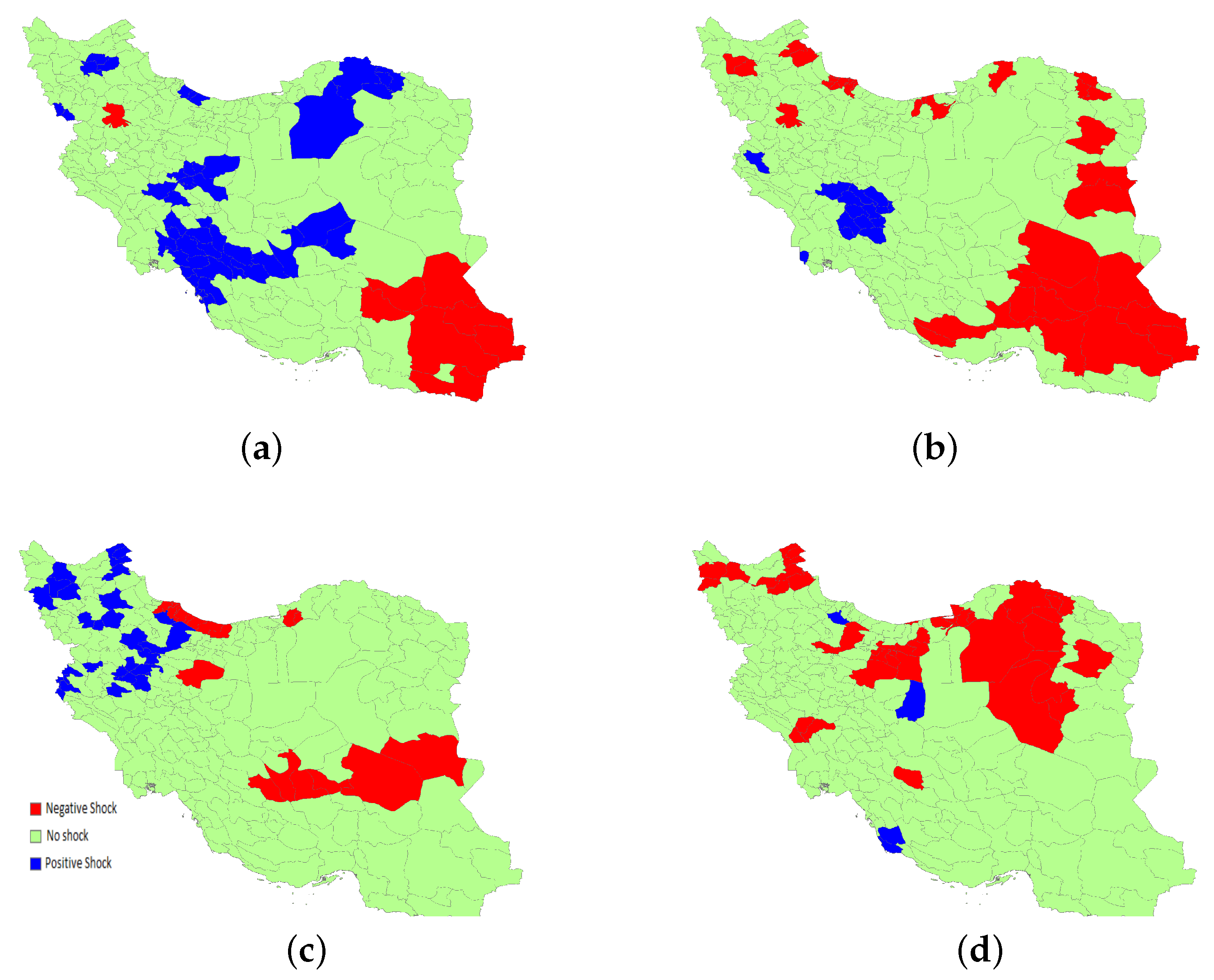
Precipitation levels dropped from the 1980s to the 2010s [49]. Yearly precipitation, which averaged about 400 mm in the period 1980–1984, declined to 320 mm in 2010–2014 (see Figure 3). During most of the focus period in this study, 2003–2014, rainfall was below its long-run average, with relatively higher levels during 2004–2008. In addition, the weather became more volatile over the same period. Figure 4 shows the five-year moving average of the percentage of the country’s area that observed a positive or negative shock. Shocks to precipitation, especially negative shocks, have become more frequent in recent years. In the 1980s, the percent area of the country affected by negative shocks was well below 20 percent. This number has increased in recent years, and was above 25 percent in the 2000–2002 and 2011–2012 periods. Predictions suggest that weather variability and shocks are likely to increase even more in the foreseeable future [50]. The distribution of shocks in selected years during the study period is depicted in Figure 5. As can be seen, different types of shocks occur in different years, especially in those districts in the northern, central, and southwestern parts of the country.

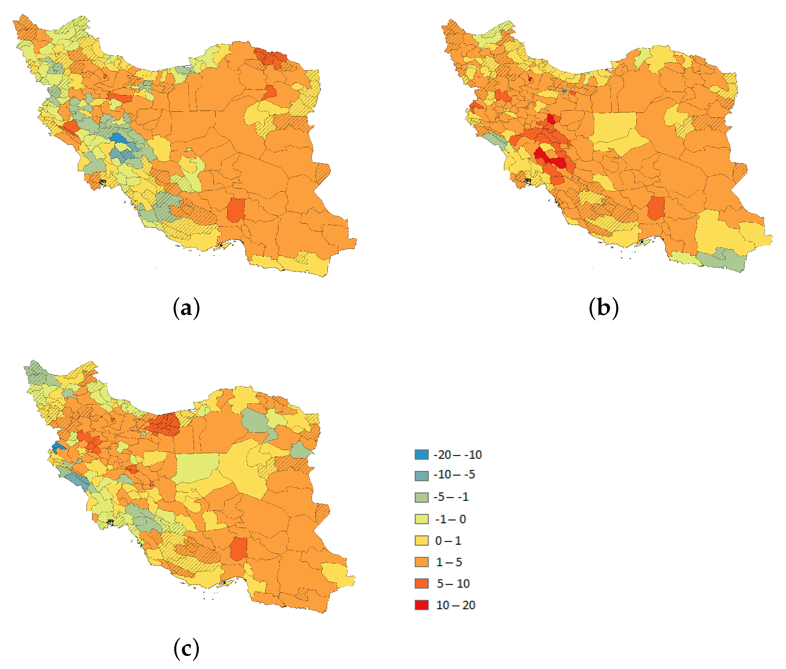
As it is located in an arid region of the world, Iran has a rainfall that is lower than the world average. Low rainfall has made agriculture in Iran very dependent on irrigation. Nearly half of the planted area in the country was irrigated in 2014, and more than 91% of rural agglomerations used wells for irrigation. In recent decades, wells have been used more intensively in response to the increased demand for water. The number of wells in the country increased from 468,049 in 2003 to 788,514 in 2014 (Iran Water Resource Management Company, Tehran, Iran 2019). This increase in the number of wells, together with prolonged droughts, resulted in a decrease in the water level in many districts of the country (see Figure 6) [51,52].

3.2. Identification Strategy

The main hypothesis of this paper is that, under the same conditions, owners of new wells will extract more groundwater than the presumably more experienced owners of older wells. The data employed include both district-level aggregated data and well-level data. These aggregated data are then used to form panel data and employ a fixed-effects model. The well-level data allow us to study the behavior of individual extractors using regression-based and matching estimators.

3.2.1. Panel Data Fixed Effects

Here, a panel data fixed-effects model is employed to estimate the relationship between the growth of new wells and extraction at the district level, as follows:

$$Y_{it}={\alpha }_0+{\alpha }_{1}WellGrowt{h}_{it}+{\mathit{\beta }}^{\prime }{x}_{it}+{\gamma }_t+{\theta }_i+{ϵ}_{it},$$

(1)

where $Y_{it}$ is the outcome of interest for district i in year t. The outcomes are measures for groundwater extraction and planted area. The six measures employed are as follows: total extraction, extraction per well, and extraction per unit of surface (km²) are used to measure for extraction, and total planted area, the ratio of planted area, and the number of planted farms are used to measure the planted area. $WellGrowt{h}_{it}$ is the growth rate in the number of wells in district i in year t, and ${\gamma }_t$ and ${\theta }_i$ are the year and district fixed effects, respectively. This model allows us to find the relationship between the growth of wells (the rate by which new wells are dug) and extraction at the district level by estimating the parameter ${\alpha }_1$.

The parameter $x_{it}$ includes four sets of control variables. The first set consists of weather-related control variables, including precipitation shocks (negative and positive) in this year, the number of positive and negative shocks in the past three years (for those areas that did not experience mixed shocks in the past three years), and yearly temperature with three lags. The second set of control variables includes variables that present district-level agricultural activities, including share and the total amount of agricultural land, ratio of gardens to agricultural land, ratio of irrigated land, the share of land used for wheat production and share of irrigated wheat production, the total population, and the ratio of rural population to total population. The third set of control variables includes the ratio of irrigated land and the share of land used for wheat production. Finally, $x_{it}$ includes control variables for the number of wells per km², the growth rate of wells (new wells/total number of wells), and a dummy variable that indicates whether a particular district split into two or more districts or not during the panel data years.

3.2.2. Double-Difference Method

The district level estimates, as explained in Section 4 below, show that districts with higher shares of newly established wells have more groundwater extraction. The next step in our empirical investigations is to find whether this is associated with the extraction behavior of new wells rather than merely a positive correlation between digging wells and high extraction in areas with ample groundwater. In order to establish the relationship between new wells and extraction, we employ several methods using the well-level data. First, the disaggregated well data in the following least-squares model is estimated:

$$Y_{it}={\alpha }_0+{\alpha }_{1}PosShoc{k}_{it}+{\alpha }_{2}NegShoc{k}_{it}+{\alpha }_{3}NewWel{l}_{it}+{\mathit{\beta }}^{\prime }{x}_{it}+{\gamma }_t+{ϵ}_{it},$$

(2)

where $Y_{it}$ is the yearly extraction (total extraction or extraction for agricultural purposes) of well i in year t and $NewWel{l}_{it}$ is an indicator which is equal to 1 if the well was dug after the start of the last calendar year.

In this model, $x_{it}$ is a vector that includes four sets of control variables. First, weather-related variables include precipitation, positive and negative shocks (defined based on precipitation), and temperature. While all regressions control for temperature, we included only precipitation or shocks related to precipitation in each regression. Here, a new variable is defined, namely, the number of positive (negative) precipitation shocks in the past three years for those wells which did not previously experience a negative (positive) shock in the same period. Second, we introduce a control for well/farm-specific variables such as irrigation method, the flow of water, availability of a water meter, existence of a water tank, depth, elevation, slope, distance to the nearest city, number of wells in a 10 km radius, area of the farm, and type of crop. With respect to the output of farms, an indicator for each crop, including wheat, rice, vegetable, oilseeds, saffron, fruit, nuts, other cereal, tea, and cotton are controlled for. The rationale for controlling for the type of crop in these models is that it has been shown that farmers who have access to groundwater change their crop type and often make it more water-intensive [53,54,55]. Third, we control for the number of seasons that the well is working, share of agriculture and industry in the total province in terms of value added in the specific survey year, and year and district fixed effects. Finally, interaction terms are included for the aquifer indicator and type of output (wheat, rice, vegetables), the log of elevation, well age, and depth. These four categories of control variables are present in all of the models; however, to preserve space, only a shorter version of the tables containing variables of interest is presented in this paper.

A double-difference framework improves the above model by comparing the difference in extraction at locations with no shock to the same difference for locations with positive (or negative) precipitation shock. Assuming that the unobserved heterogeneity between new and old wells due to factors such as better equipment, more efficient depth, etc. is fixed over time, the first difference captures the non-behavioral difference in well yields. It is not expected that the difference in the delivery from new and old wells due to these unobserved factors will change as other determinants (such as weather shocks) vary. The double-difference method benefits from the exogenous variation in shocks to identify the difference in extraction from new wells compared to that of old wells when they are exposed to precipitation shocks. This model can be shown with the equation below:

$$\begin{array}{cc}\hfill & Y_{it}={\alpha }_0+{\alpha }_{1}PosShoc{k}_{it}+{\alpha }_{2}NegShoc{k}_{it}+{\alpha }_{3}NewWel{l}_{it}+\hfill \\ \hfill & {\alpha }_{4}NewWel{l}_{it}\times PosShoc{k}_{it}+{\alpha }_{5}NewWel{l}_{it}\times NegShoc{k}_{it}+{\mathit{\beta }}^{\prime }{x}_{it}+{\gamma }_t+{ϵ}_{it}.\hfill \end{array}$$

(3)

In this model, the coefficients of interest are the interaction terms of new well and shocks; ${\alpha }_5$ shows the difference in the extraction of new and old wells in regions that experienced negative precipitation shock compared to regions that did not experience any shock, while ${\alpha }_4$ is interpreted in a similar manner when positive precipitation shocks are considered.

3.2.3. Nearest-Neighbor Matching

The regression analysis defined above compares the average extraction of new wells with older ones while controlling for observable characteristics and unobservable location and time effects. The identification in this model results from the exogenous variation in shock exposure, which allows us to identify the difference in the behavior of new wells, while a matching estimator allows us to calibrate the counterfactual selection for new wells. A nearest-neighbor matching method is used to find the average treatment effect on the treated (ATT), in which the treatment variable is the indicator for new wells. Using a distance function, new wells are matched to the closest old wells (comparison group). The comparison groups are chosen based on well-specific variables (such as depth, flow of water, etc.), farm characteristics (such as planted area, crop type, etc.), weather variables (such as average temperature, positive and negative precipitation shocks, etc.), and province-level characteristics (such as total and share of the agricultural sector’s value added).

An advantage of using the nearest-neighbor matching method over regression-based models is that comparison wells can be found that are very similar to new wells in terms of location-related attributes such as weather and soil characteristics by using a weighting scheme that places a larger weight on geographical location in the distance function. Likewise, the weight for the water flow of wells can be raised to control for unobserved heterogeneity that may exist due to equipment and hydrological variations, thereby removing potential bias. In all of the specifications in Section 4.3, the bias-adjusted matching estimator proposed by Abadie and Imbens [56] is employed.

4. Results

The estimation results are presented in the following three subsections. First, in Section 4.1, the findings when estimating Equation (1) using the panel of agricultural censuses are presented. In Section 4.2, the results from estimating the census of wells using Equations (2) and (3) are shown. In Section 4.3, the results from the matching estimator are discussed. For a more extensive discussion of our results, including robustness checks, please see Appendix A.

4.1. Panel Data Estimations

In this section, the estimation results from a panel fixed-effects model based on the agricultural censuses collected by the SCI in 2003 and 2014 are presented. The regression model employed here is Equation (1); the total extraction from wells, extraction per well and per unit of surface (km²), and their logarithmic (Ln) forms are used as the dependent variables. Moreover, the models include four sets of control variables for all models, as described in Section 3.2.

Table 3. Estimates of the effect of growth in wells on extraction, extraction per well, and extraction per unit of surface, panel data.

	Extraction			Ln of Extraction
	(1)	(2)	(3)	(4)	(5)	(6)
	Total	Per Well	Per Surface	Total	Per Well	Per Surface
Growth in # of wells	−22.062	0.240 ***	15.514 **	0.004 ***	0.004 ***	0.006 ***
	(85.107)	(0.085)	(6.749)	(0.002)	(0.001)	(0.002)
Positive precipitation shock	3263.591	−1.589	128.189	0.045	0.101	0.003
	(11,232.060)	(11.268)	(890.745)	(0.199)	(0.084)	(0.200)
# of positive precipitation shock in past 3 years	4117.709	−18.251 *	299.769	−0.069	−0.040	−0.023
	(9657.650)	(9.689)	(765.889)	(0.171)	(0.072)	(0.172)
Negative precipitation shock	−10,112.267	25.668 **	−752.664	−0.326	0.223 ***	−0.330 *
	(11,204.307)	(11.241)	(888.544)	(0.198)	(0.084)	(0.199)
# of negative precipitation shock in past 3 years	2115.660	−4.616	352.995	0.067	−0.145 ***	0.072
	(4584.084)	(4.599)	(363.535)	(0.081)	(0.034)	(0.082)
$R^2$	0.192	0.451	0.173	0.117	0.637	0.159
Observations	598	598	598	598	598	598

Notes: Dependent variables are extraction, extraction per well, extraction per unit of surface (km²), and their log forms. Standard errors are in parentheses. * p < 0.10, ** p < 0.05, *** p < 0.01. Source: Statistical Center of Iran and Iran Water Resource Management Company (2003–2014).

provides the estimation results of a fixed-effects model, with the dependent variables being total extraction, extraction per well, and extraction per unit of surface (km²). In columns 4–6, the dependent variables are those of columns 1–3 in their log form. Total extraction is the total amount of extraction from all wells in each district of Iran. None of the reported variables in the table are statistically significant for total extraction (column 1). The distribution for total extraction is highly skewed, as is the distribution for the other two dependent variables in this table. Therefore, we use the log form of the dependent variables in the models (columns 4–6).

The main variable of interest is the rate of growth in the number of wells. As can be seen, the coefficient of the growth rate in the number of wells is positive and statistically significant in all models except for (1). For the log of total extraction, this significance is a trivial result; if there are more wells, they collectively extract more water. However, for extraction per well and extraction per unit of the area this positive relationship raises three main possibilities. First, new wells systematically extract more water than the old wells, and that is why a positive change in the number of wells increases extraction per well. Second, new wells are dug in areas with larger water availability. Third, establishing new wells raises the competition among all wells in the region, and all of them start extracting more water. In Section 4.2 and Section 4.3, supportive evidence is provided to indicate that the first possibility is the most plausible one.

Another interesting finding is the reaction of farmers in terms of their agricultural activities to weather shocks at the district level. In an arid area such as Iran, farmers shield their business by employing groundwater.

Table 4. Response of agricultural activity to precipitation shocks.

	(1)	(2)	(3)
	Ratio Planted	Total Planted Area (Ha)	# of Planted Farms
Growth in # of wells	0.000	11.184	0.030
	(0.000)	(18.156)	(2.568)
Positive precipitation shock	0.036 **	2521.723	171.659
	(0.018)	(2308.428)	(326.509)
# of positive precipitation shock in past 3 years	−0.006	1750.907	613.141 **
	(0.016)	(2061.176)	(291.537)
Negative precipitation shock	−0.051 ***	−6046.670 ***	−550.130 *
	(0.017)	(2251.919)	(318.516)
# of negative precipitation shock in past 3 years	−0.001	608.177	−1.759
	(0.007)	(955.851)	(135.198)
$R^2$	0.433	0.185	0.300
Observations	598	598	598

Notes: The dependent variables are the ratios of planted area, total planted area, and number of planted farms. Standard errors are shown in parentheses. * p < 0.10, ** p < 0.05, *** p < 0.01. Source: Statistical Center of Iran and Iran Water Resource Management Company (2003–2013).

presents three variables that indicate the level of agricultural activities. The ratio planted is the ratio of farm land (farm or garden) to the amount of arable land (column 1). In other words, it distinguishes between the amounts of fallow and planted land. The results show that negative precipitation shocks reduce the ratio of planted land. Considering that a large share of agriculture in Iran is rain-fed, it is obvious that a negative precipitation shock decreases the amount of land that farmers cultivate. The total planted area (farm land), the dependent variable for the model in column 2, is the numerator of the previous index. The result of this model is consistent with the previous model (column 1). The number of planted farms is another useful index. Small land ownership is a common phenomenon in Iran, and column 3 shows that more positive precipitation shocks increase the number of farms under cultivation. In [7], the authors found an more extensive version of these same results by examining the effect of climatic variables on demand for water, crop selection, shares of different crops, and adoption of technology using a variety of model specifications and climate variables.

4.2. Well Level Estimations

In the previous section, three possibilities were mentioned for the positive relationship between the number of wells and extraction per well, along with the number of wells and extraction per unit of area. This section explains that this positive relationship exists because the new wells systematically extract more water than the old wells. Moreover, this section provides more evidence for the main hypothesis of this paper.

The models are first estimated based on Equation (2). There are two main dependent variables, namely, total extraction from each well in each year and the amount of extracted water used for agricultural purposes. The same models are estimated with these dependent variables in their log forms. Before explaining the results, the regression setup and dependent variables are provided here. The models are estimated using the data for wells that were active during the survey years and were at least partially used for agricultural activities. Moreover, because the hypothesis is based on the age of wells, the wells for which either the survey year or the establishment year was missing were excluded. All of our regressions use four sets of control variables, as discussed in Section 3.2. Finally, district-level clustered standard errors are reported for all estimations in parentheses.

Table 5. Extraction behavior and its difference between new wells and old wells.

	Extraction		Ln of Extraction
	(1)	(2)	(3)	(4)
	Total	Agriculture	Total	Agriculture
Newly established well	5435.571 **	5819.657 **	0.115 ***	0.129 ***
	(2538.740)	(2535.759)	(0.031)	(0.034)
Positive precipitation shock	−10,214.989	−9621.044	0.066	0.079
	(8019.298)	(7906.265)	(0.095)	(0.094)
Negative precipitation shock	6537.964	6216.317	0.011	−0.010
	(5073.722)	(5154.745)	(0.057)	(0.061)
# of positive precipitation shock in past 3 years	656.955	819.376	0.103 *	0.129 **
	(6743.547)	(6649.742)	(0.059)	(0.061)
# of negative precipitation shock in past 3 years	−8400.560 *	−8704.855 *	−0.084 **	−0.116 **
	(4629.733)	(4520.307)	(0.041)	(0.047)
# of wells in 10 km radius	1118.377	1295.680	−0.076 ***	−0.070 ***
	(1453.931)	(1448.999)	(0.015)	(0.015)
Adjusted $R^2$	0.723	0.720	0.867	0.863
Observations	395,321	395,321	395,321	395,321

Notes: All regressions are based on Equation (2). Dependent variables are total extraction, extraction for agricultural purposes, and their log forms. District level clustered standard errors are shown in parentheses. * p < 0.10, ** p < 0.05, *** p < 0.01. Source: Iran Water Resource Management Company (2003–2013).

shows that the owners of new wells are able to extract more water compared to the owners of old wells. This holds at both the level and log form of the dependent variable, and for both total extraction and extraction for agricultural purposes. In terms of magnitude, in the models in columns 1 and 2 the extraction from a newly established well is 6.2 and 6.7 percent more than that of an old well for total extraction and extraction for agriculture purposes, respectively (the mean extraction for total extraction is 88,036 m³, while for extraction for agriculture purposes it is 87,061 m³). Considering the models with the dependent variables in their log forms (columns 3 and 4), the extraction is 11.5 and 12.9 percent higher for new wells. Previous studies have found that farmers change their crops when they use groundwater in a way that increases their water consumption [53,54,55]. In these models, therefore, controls for the type of crop are included in order to capture the effect of crop selection.

A positive or a negative shock in the current year does not affect extraction in a statistically significant way. However, the number of negative shocks in the past three years reduces extraction as measured by all four models. For the models with the dependent variable in the log form, positive shocks in the past three years increase extraction. In light of the results shown in Table 4, negative precipitation shocks encourage farmers to plant smaller areas of land. As farmers plant less land, they extract less water from wells.

As explained in Section 3.2.2, the double-difference model in Equation (3) can be used to remove potential omitted variable bias in the least-squares model used above.

Table 6. Extraction behavior and its difference between new wells and old wells: double-difference method.

	Extraction		Ln of Extraction		Extraction		Ln of Extraction
	(1)	(2)	(3)	(4)	(5)	(6)	(7)	(8)
	Total	Agriculture	Total	Agriculture	Total	Agriculture	Total	Agriculture
Positive precipitation shock	−10,271.837	−9681.910	0.064	0.077	−9998.250	−9404.882	0.065	0.078
	(8025.781)	(7913.092)	(0.095)	(0.094)	(8029.682)	(7916.151)	(0.095)	(0.094)
Negative precipitation shock	6423.347	6093.601	0.008	−0.013	6945.864	6623.522	−0.000	−0.022
	(5078.667)	(5160.731)	(0.057)	(0.061)	(5064.222)	(5142.992)	(0.057)	(0.061)
# of positive precipitation shock in past 3 years	730.908	898.555	0.105 *	0.131 **	720.217	882.445	0.104 *	0.130 **
	(6743.425)	(6650.105)	(0.059)	(0.061)	(6746.217)	(6652.600)	(0.058)	(0.061)
# of negative precipitation shock in past 3 years	−8439.685 *	−8746.744 *	−0.085 **	−0.117 **	−8373.909 *	−8678.256 *	−0.085 **	−0.116 **
	(4642.467)	(4533.963)	(0.041)	(0.048)	(4630.739)	(4521.278)	(0.041)	(0.047)
# of wells in 10 km radius	1133.065	1311.406	−0.075 ***	−0.069 ***	1121.476	1298.772	−0.076 ***	−0.070 ***
	(1454.569)	(1449.797)	(0.015)	(0.015)	(1453.987)	(1449.018)	(0.015)	(0.015)
Newly established well					9268.505 ***	9644.523 ***	0.048	0.060 *
					(2764.729)	(2784.481)	(0.032)	(0.032)
Newly established well × Negative precipitation shock = 1					−8075.121	−8062.710	0.251 ***	0.270 ***
					(4588.077)	(4624.741)	(0.088)	(0.095)
Newly established well = 1 × Positive precipitation shock = 1					−12,392.132 ***	−12,357.374 ***	0.010	−0.012
					(3769.745)	(3728.093)	(0.048)	(0.050)
Adjusted $R^2$	0.723	0.720	0.867	0.863	0.723	0.720	0.867	0.863
Observations	395,321	395,321	395,321	395,321	395,321	395,321	395,321	395,321

Notes: All regressions are based on Equation (3). Dependent variables are total extraction, extraction for agricultural purposes, and their log forms. District level clustered standard errors are shown in parentheses. * p < 0.10, ** p < 0.05, *** p < 0.01. Source: Iran Water Resource Management Company (2003–2013).

shows that the owners of new wells extract even more when they experience a negative precipitation shock. The first four columns of this table are the same as Table 5, except that they do not have the dummy variable for a new well. Columns 5 to 8 are the same as Table 5 as well, except that, other than the indicator for new well, they include interaction terms between the new well and precipitation shock indicators. Looking at columns 5 and 6, it is evident that extraction from newly established wells is higher than older wells in general, although this difference becomes smaller when there is a positive precipitation shock. Moreover, columns 7 and 8 show that, in log form, extraction from new wells is again higher than from old wells, and the owners of new wells extract even more when there is a negative precipitation shock.

One important question that is investigated in this paper is how long it takes for owners of wells to adapt to new technology. In other words, it is interesting to examine whether the results change when extraction from wells of different ages is compared. For example, do the owners of a two-year-old well extract more than their counterparts with older wells? Or, is extraction from three-year-old wells higher than for older wells? An answer for this question can be provided by estimating Equation (2), where a comparison is made between the extraction of wells of a specific age and their older counterparts.

Table 7. Changing the definition of new wells and its effect on the difference in extraction of new wells and old wells.

	Ln of Extraction
	(1)	(2)	(3)	(4)	(5)	(6)	(7)	(8)
	Total	Total	Total	Total	Agriculture	Agriculture	Agriculture	Agriculture
2-year old	0.050 *				0.047
	(0.027)				(0.029)
3-year well		−0.039				−0.038
		(0.025)				(0.024)
4-year well			0.006				0.007
			(0.021)				(0.021)
5-year well				0.000				0.001
				(0.013)				(0.013)
Adjusted $R^2$	0.869	0.869	0.869	0.871	0.865	0.865	0.866	0.867
Observations	379,488	368,769	355,891	342,496	379,488	368,769	355,891	342,496

Notes: Dependent variables are the log forms of total extraction and extraction for agricultural purposes. District-level clustered standard errors are shown in parentheses. * p < 0.10. Source: Iran Water Resource Management Company (2003–2013).

shows that none of the owners of wells that are three, four, or five years old extract significantly more water than those who own older wells. The coefficient for two-year-old wells is statistically significant only at the 10% level for total extraction (column 1), and is not significant for extraction for agricultural purposes (column 5). Only the models with the log forms of the dependent variable are included in this table. However, using the levels of the dependent variables does not change the general picture. As can be seen in the table, all coefficients are insignificant, and there is no specific pattern in these figures. One implication of these findings is that learning happens quickly, resulting in the coefficients of variables of wells that are two, three, four, and five years old becoming statistically insignificant.

Another interesting outcome is to test whether learning continues to take place after the first year of adoption. The coefficients found thus far are the differences between the behavior of new wells and the average behavior of wells of different ages. The question is whether the results stay the same if one compares new wells with wells of a certain age. This comparison is presented in

Table 8. Difference in extraction from new wells and old wells for different groups of old wells by age.

	Ln of Total Extraction					Ln of Extraction for Ag Purposes
	(1)	(2)	(3)	(4)	(5)	(6)	(7)	(8)	(9)	(10)
	2 Years	5 Years	8 Years	10 Years	30 Years	2 Years	5 Years	8 Years	10 Years	30 Years
Newly established well	0.044	0.078 *	0.079 **	0.086 ***	0.101 ***	0.053 *	0.086 **	0.086 **	0.096 ***	0.116 ***
	(0.027)	(0.042)	(0.033)	(0.029)	(0.030)	(0.029)	(0.042)	(0.033)	(0.030)	(0.032)
Positive precipitation shock	0.321 ***	0.292 ***	0.197 **	0.202 **	0.062	0.350 ***	0.315 ***	0.216 **	0.221 **	0.076
	(0.108)	(0.097)	(0.095)	(0.090)	(0.093)	(0.108)	(0.096)	(0.093)	(0.090)	(0.092)
Negative precipitation shock	0.139 *	0.112	0.085	0.058	0.009	0.119	0.086	0.057	0.036	−0.011
	(0.079)	(0.074)	(0.069)	(0.065)	(0.059)	(0.082)	(0.080)	(0.075)	(0.071)	(0.063)
Adjusted $R^2$	0.876	0.855	0.866	0.867	0.869	0.873	0.851	0.863	0.864	0.865
Observations	26,552	68,320	117,688	157,966	357,649	26,552	68,320	117,688	157,966	357,649

Notes: Dependent variables are log forms of total extraction, and extraction for agricultural purposes. District level clustered standard errors in parentheses. * p < 0.10, ** p < 0.05, *** p < 0.01. Source: Iran Water Resource Management Company (2003–2013).

by re-estimation of Equation (2) and restricting well age. The dependent variable for the first five columns is the log of total extraction, and the dependent variable for the next five columns is the log form of extraction for agricultural purposes. In each column, the indicator for a new well is kept as before and the well age is restricted to two, five, eight, ten, or thirty years old. The comparison of new wells with two-year-old wells (column 1) shows no difference in total extraction from these wells. In column 6, extraction for agricultural purposes is used as the dependent variable; the difference between new wells and two-year-old wells is significant only at the 10% level. For other age limits (five to thirty) the difference in extraction is statistically significant. As can be seen, the difference in extraction increases, and remains significant as the age limit is increased. The results presented in Table 7 and Table 8 can thus represent a guide to the learning duration. These results indicate that learning requires at least two years to take place. With this table, a comparison can be made between these results and the original results in Table 5. As the age limit increases in the results presented in Table 8, the coefficients for the new well indicator approach those in Table 5.

One might wonder whether new wells have an advantage in location compared to their older counterparts. In other words, if new wells appear only in locations with better access to groundwater, the results might be driven by a bias toward access to water sources, or by superior location. Numerically, the percentage of new wells in each province is presented in

Table 9. Comparison of new and old wells by province.

Province Name	Old Wells			New Wells
	Depth	Nearest Well (m)	# of Wells in 10 km	Depth	Nearest Well (m)	# of Wells in 10 km	New Well (%)
Alborz	50.94	102.29	76.31	52.24	122.75	91.30	2.28
Ardebil	8.92	366.01	3.47	8.40	513.18	4.70	4.44
Bakhtiari	58.76	315.17	5.77	50.07	304.81	8.44	0.91
Bushehr	29.78	186.47	21.58	32.05	219.64	23.30	1.20
E.Azarbaijan	28.93	170.71	51.75	39.43	176.95	64.94	2.61
Fars	60.39	220.53	16.95	81.17	185.14	41.05	4.38
Gilan	11.52	101.17	55.47	14.71	110.86	67.38	7.91
Golestan	37.90	163.47	33.42	60.39	130.69	61.83	1.99
Hamadan	56.58	354.51	8.44	54.80	285.48	19.86	3.08
Hormozgan	35.69	206.50	19.71	45.52	253.56	21.48	1.08
Ilam	52.28	469.86	3.50	36.30	520.68	4.40	4.90
Isfahan	53.18	179.78	59.90	67.88	196.31	105.81	2.68
Kerman	68.13	351.06	14.59	95.36	551.39	14.05	1.69
Kermanshah	43.65	250.46	14.07	46.08	227.53	25.32	4.98
Khorasan Razavi	72.88	467.63	15.74	21.75	128.17	113.06	6.16
Khuzestan	41.19	288.60	12.81	16.78	180.28	35.07	15.11
Kohkiloyeh	32.60	206.05	12.58	28.56	342.04	11.69	5.59
Kurdestan	33.27	322.40	8.84	28.45	274.18	16.92	5.11
Lorestan	51.91	358.12	4.14	36.89	277.72	8.44	10.19
Markazi	61.65	368.45	6.14	56.02	317.97	13.96	1.68
Mazandaran	16.61	75.65	90.33	19.70	88.27	128.13	3.31
N. Khorasan	54.68	488.27	7.27	31.69	374.96	12.38	1.01
Qazvin	75.49	383.58	8.69	61.86	299.21	24.58	6.61
Qom	47.26	322.24	17.05	57.28	374.95	25.52	3.19
S. Khorasan	88.33	869.94	0.79	80.57	776.62	1.63	0.53
Semnan	105.18	488.73	5.89	77.80	467.04	5.75	0.91
Sistan and Baluchestan	26.78	347.97	8.22	27.14	377.32	10.00	0.92
Tehran	50.82	111.43	88.89	41.97	101.85	168.06	2.53
W.Azarbaijan	20.32	108.51	50.57	24.16	110.15	70.72	6.44
Yazd	102.55	691.61	1.50	125.86	737.42	2.33	3.06
Zanjan	31.44	211.30	18.46	29.96	196.83	32.24	4.46

Source: Iran Water Resource Management Company (2003–2013).

. The ratio is small, below seven percent, with only two exceptions, namely, Khuzestan and Lorestan provinces, which have high ratios of new wells. Both of these provinces have small numbers of wells (5958 and 2642, respectively), and a few new wells therefore creates a big jump in the ratio of new wells. The distribution of new wells inside each province is examined as well. New and old wells are distributed very closely to each other. The mean distance of the nearest well varies from 75 m to 870 m for old wells and from 88 m to 777 m for new wells. Moreover, there are multiple wells in a 10 km radius of both new wells and old wells (see Table 9). Another important factor in determining extraction is the type of crop. In the sample, a comparison is made between the type of crop for new and old wells.

Table 10. Share of new and old wells by crop type (%).

	Wheat	Rice	Other Cereals	Vegetables	Fruits
Newly established wells	24.9	27.3	19.3	14.3	23.8
Old wells	24.1	23.4	22.6	16.6	23.2

Note: Farmers may plant more than one type of crop. Source: Iran Water Resource Management Company (2003–2013).

shows the percentage of new and old wells used for wheat, rice, other cereals, vegetables, and fruits. The percentages of wells that are used to water wheat, vegetables, and fruits are very close between new and old wells.

4.3. Nearest-Neighbor Matching

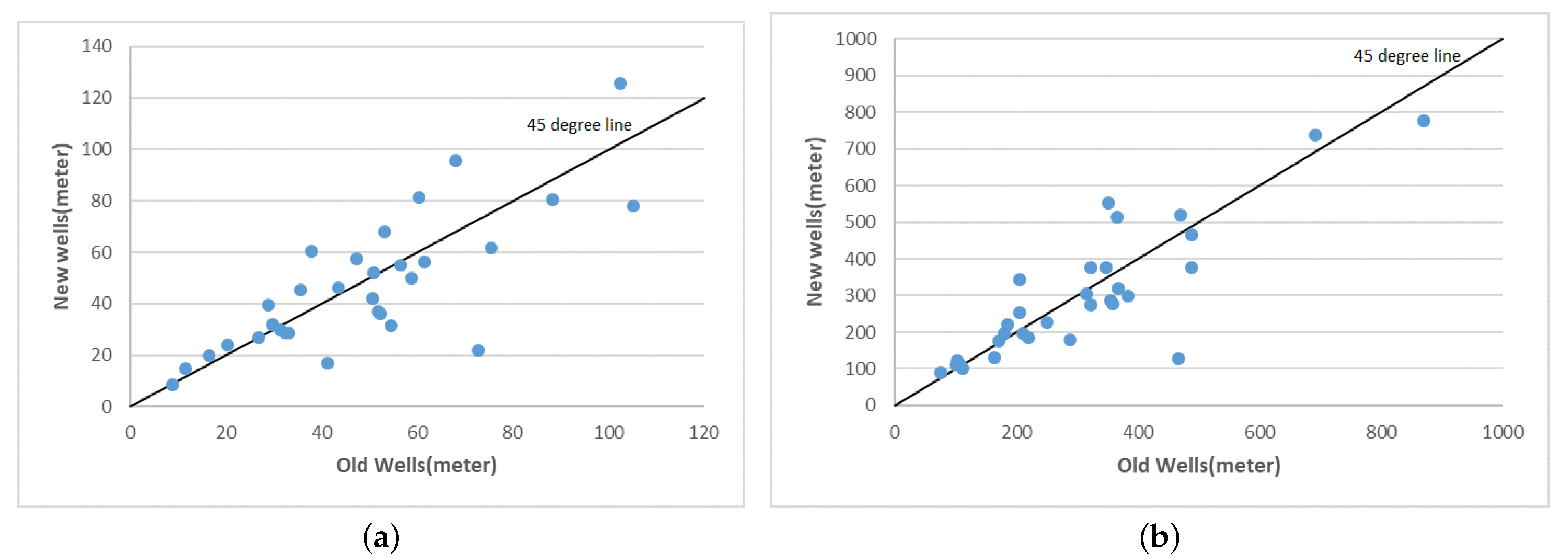
In this section, the focus is on the difference in extraction behavior between new and old wells using nearest-neighbor matching. This matching model is useful for comparing the extraction from new wells with that from old wells which are very similar or exactly the same in terms of their location-specific and well-specific attributes. In addition, this section discusses how the models can be modified in order to better control for unobservable factors. As previously discussed, new wells do not have visible advantages over old wells in terms of location and availability of water. New and old wells in each province have similar characteristics, as shown in Table 9 and discussed in detail in Section 4.2. Figure 7 shows that the depth and the distance to the nearest well are very close for both new and old wells in the provinces. The solid lines in both subfigures of this figure are 45 degree lines. If a point falls on these lines, it reflects that the depth or the distance to the nearest well is the same for new and old wells, on average, in the associated province. This distribution shows that a high degree of common support exists for the wells compared in this study. In the matching models, new wells are considered ‘treated’, and at least four matches are found for each of them among the old wells (control group). ATT (average treatment effect on the treated) is then computed based on these matched wells.

In the baseline model (Matching Model I), the Mahalanobis distance measure is employed as the preferred metric [57,58]. The covariates used as proximity variables are the flow of water, longitude, latitude, planted area, well age, elevation, slope, distance to the nearest city (km), number of wells in a 10 km radius, distance to the closest well, share of industry value added from the province’s total value added, share of agriculture value added, average temperature and its three lags, and indicators for water meter, reservoir, irrigation method, prohibited drilling zones, and type of crop. The variables used for exact matches are positive and negative precipitation shocks, the number of positive and negative precipitation shocks in the past three years, and the number of working seasons. As the exact matching and proximity variables here indicate, similar variables to the ones used in the regression analysis are employed, leading to an important improvement. In this model, longitude and latitude can be included as proximity variables. By employing these criteria, for 13,388 out of 13,390 of the new well at least four matches are found among the control group. The matching estimates were adjusted for potential bias following [56]. The bias adjustment regressions include all variables used in the distance function except for those in the exact match.

The baseline model (Matching Model I) produces very close matches for new and old wells in the sample.

Table 11. Summary statistics of match quality for Matching Model I.

Difference In	Mean	Std. Dev.	Min.	Max.	% with Zero
Water flow	−0.041	5.596	−65	61.26	17.35
Depth	−1.189	24.009	−260	315	11.92
Age	2.558	2.954	1	53
Distance	0.19	0.707	0	13.111
Latitude (X)	−0.021	0.563	−11.54	10.124
Longitude (Y)	0.025	0.466	−9.704	10.41
Year	0	0	0	0	100
Positive shock	0	0	0	0	100
Negative shock	0	0	0	0	100
# of positive shock in past 3 years	0	0	0	0	100
# of negative shock in past 3 years	0	0	0	0	100
# of season worked	0	0	0	0	100
N	53,552

Note: A test for significant differences in mean between treatment and control groups was performed for each of the variables above. Tests for all variables failed to reject the hypothesis that the means are equal at 1%, 5%, and 10% significance levels.

provides summary statistics to evaluate the quality of matching. There is no discrepancy between the year and the number of seasons worked, and all of the wells have the same status in terms of weather shocks. This is not surprising, as these variables were set to be exactly matched. The mean distance between the peers is very low, only 21 km, as is the latitude and longitude of the matches. The difference between water flow is very small; 17% of matched wells have the same water flow as the new wells they are matched to, and the average difference is only 0.041 m³/s. The same is true for depth; for almost 12% of the matches the difference is zero, and the average difference in depth is slightly more than one meter.

Table 12. Nearest-neighbor matching estimates of the difference in extraction, baseline model.

	Total Extraction	Extraction for Agriculture
	(1)	(2)
Mean Extraction New Wells	79,797.06	78,805.52
Mean Extraction Old Wells	72,172.8	71,623.17
ATT (1 vs. 0)
Newly established well	7624.26 ***	7182.35 ***
	(1062.63)	(1065.25)

Note: ATT is average treatment effect on treated. *** p < 0.01. Source: Iran Water Resource Management Company (2003–2013).

presents the results when matching new wells with old wells using the baseline nearest-neighbor matching method. Column 1 shows the difference between the total extraction of new and old wells. On average, new wells extract 7624 m³ more than their older counterparts, which is 10.56 percent more. These numbers are 7182 m³ and 10.03 percent, respectively, for extraction for agricultural purposes, presented in column 2. These results are well in line with the findings in the regression analysis presented in Section 4.1 and Section 4.2.

An improvement in the baseline model is possible by adjusting the matching method in such a way that new wells are matched with old wells which are very likely to have similar unobserved and unobservable characteristics. Attributes such as the geological properties, power of the pump, and effects of well age on extraction capacity are among the unobserved determinants of extraction from a well. A nearest-neighbor matching estimator can be used to account for these characteristics. Matching based on the flow of water summarizes all of these variables; if two wells can provide the same flow, they should have a combination of the above attributes that guarantees an exact yield for the well. As the flow of water is an important variable for capturing unobserved characteristics, the matches are found in such a way that they are (nearly) exactly the same based on the flow of water by raising the weight of this variable in the distance metric by a factor of one hundred. The implementation of this weighting is explained in detail in Appendix A.3 of the Appendix. As water flow captures the unobserved heterogeneity between the matched wells, a larger estimate for the extraction from new wells must be due to the behavior of the owners of these wells. Following similar logic, the weights for longitude and latitude can be raised in order to obtain matches that are geographically close to each other. In this case, the weights for longitude and latitude are increased by a factor of one hundred. This guarantees that location-specific characteristics such as weather and soil quality are very similar. This reweighted model is called Matching Model II, and is different from the baseline model only in the weights used for the flow of water and for the longitude and latitude in the distance metric.

The estimation results of Matching Model II are presented in

Table 13. Nearest-neighbor matching estimates of the difference in extraction, Matching Model II.

	Total Extraction	Extraction for Agriculture
	(1)	(2)
Mean Extraction New Wells	80,811.19	79,926.25
Mean Extraction Old Wells	74,769.33	74,024.15
ATT (1 vs. 0)
Newly established well	6041.86 ***	5902.09 ***
	(611.87)	(614.76)

Note: ATT is average treatment effect on treated. *** p < 0.01. Source: IranWater Resource Management Company (2003–2013).

. In terms of total extraction, new wells extract more than eighty thousand cubic meters of water, while old wells extract around seventy-five thousand cubic meters in one year. The difference in extraction is positive; new wells extract six thousand more cubic meters of water compared to old wells. The difference in extraction is smaller when unobservable factors are controlled for in the reweighted model. Extraction for agricultural purposes is larger for new wells compared to old wells by six thousand cubic meters. These findings confirm our previous findings using regression models and the baseline matching model.

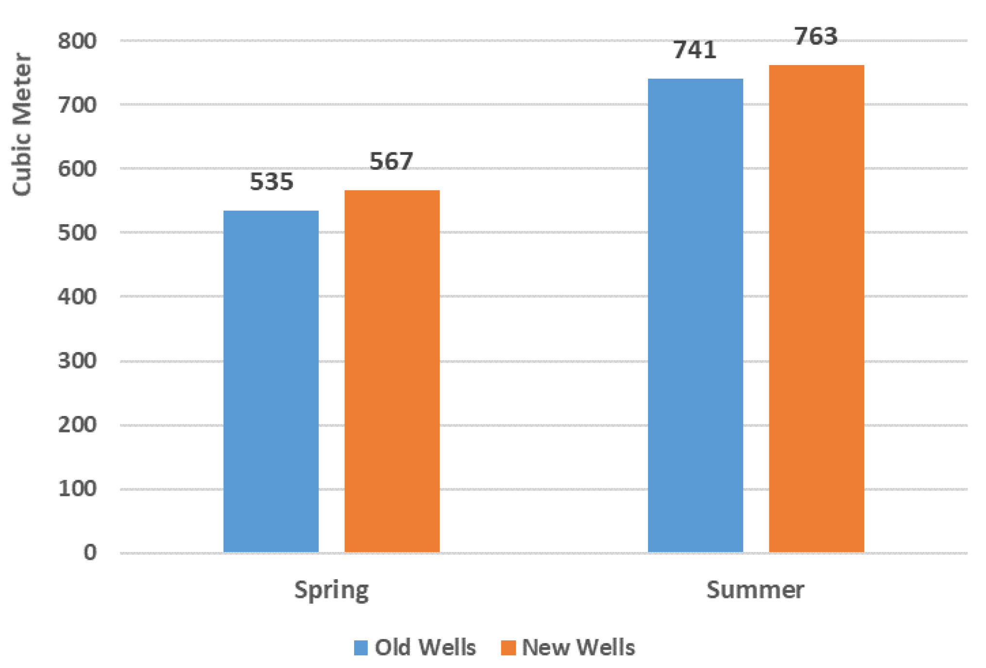
It is worthwhile to further explore whether the more aggressive extraction from new wells is due to the behavior of their owners by comparing the seasonal extraction from wells. Figure 8 shows the Spring and Summer extraction from new wells and their matched old wells. In both seasons, new wells extract more than old wells. However, old wells have the capacity to significantly increase water delivery in the Summer compared to new wells. Extraction from new and old wells increases from Spring to Summer by 34.57 and 38.50 percent, respectively. This shows that owners of older wells extract less in the Spring, while in the Summer they have more capacity to raise their extraction, presumably when they need more water due to the heat. We rigorously tested the difference in Spring–Summer extraction using our baseline and reweighted models.

Table 14. Difference in extraction between Spring and Summer.

	Baseline	Reweighted
	(1)	(2)
Mean Difference in Summer–Spring Extraction, New Wells	199.35	195.46
Mean Difference in Summer–Spring Extraction, Old Wells	204.3	205.59
ATT (1 vs. 0)
Newly-established well	−4.98	−10.12 ***
	(3.81)	(2.9)

Note: ATT is average treatment effect on treated. *** p < 0.01. Source: IranWater Resource Management Company (2003–2013).

presents the results for these models. Both models indicate that the increase in summer extraction is smaller for new wells, although the difference is only statistically significant for the reweighted model estimate. Considering that in these estimates new wells are matched to old wells with similar observable characteristics, this observed difference in extraction pattern must be due to differences in the behavior of the owners of the wells.

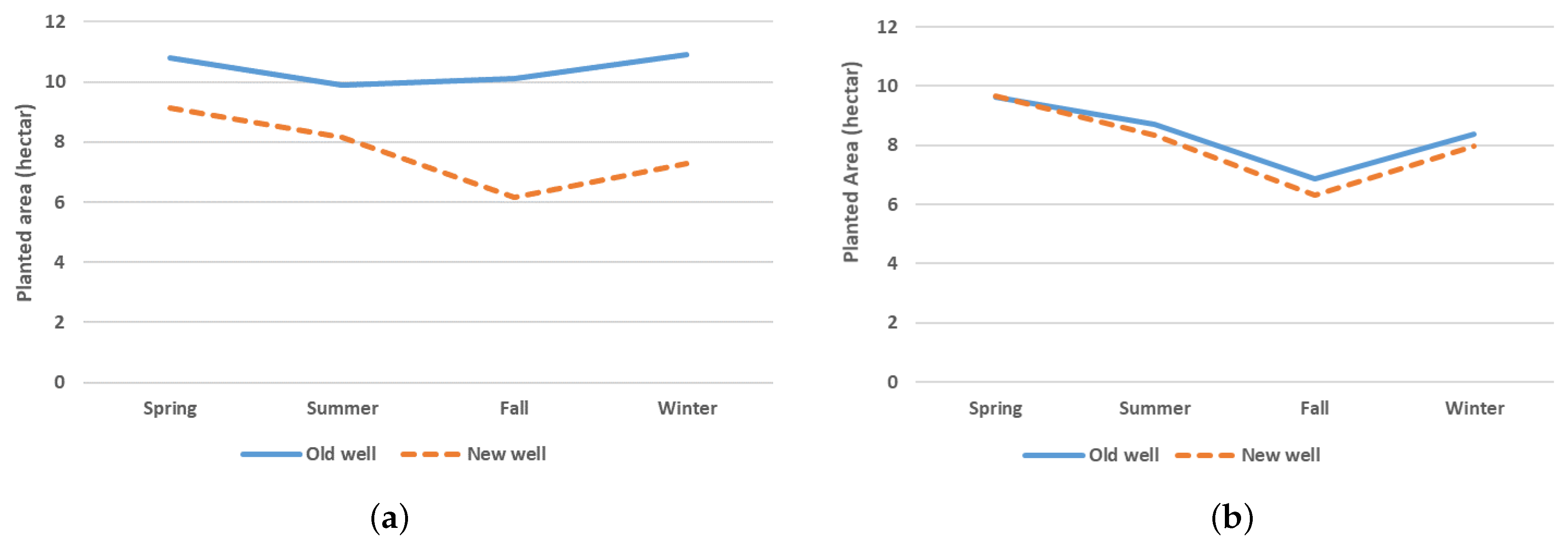
Figure 9 provides a more clear picture of the effect of experience on management of water resources. This figure provides the planted area by season for new and old wells. Panel (a) of the figure is drawn for all wells, while panel (b) is for matched wells only. Panel (a) shows that owners of old wells plant a relatively stable amount of land in different seasons (around 10–11 hectares in each season), while owners of new wells plant around 9 hectares in the Spring and their ability to maintain their planted land area decreases sharply by the Fall. On this basis, it can be claimed that with their longer experience, owners of old wells are able to distribute their water over seasons, which the owners of new wells fail to do. In panel (b), the difference between the planted area of new and old wells is smaller, as only matched wells are considered in estimates and the planted area is included in the distance function. Nonetheless, this figure shows that new well owners are not able to maintain their planted area.

5. Discussion

The results presented in Section 4 show that owners of newly established wells extract more water than experienced owners of old wells. The results from our regression model (Column 4 of Table 5) show that extraction from new wells is higher by 5820 m³ per year compared to old wells. The mean extraction is 87,061 m³ per year; thus, extraction from new wells is 6.7 percent higher than the average. The matching model provides closer estimates compared with the regression model. As shown in Table 13, extraction from new wells is higher by approximately 5902 m³ per year compared to old wells. As expected, all wells increase their extraction from Spring to Summer. However, the increase in extraction from new wells (35 percent increase) is smaller than that from old wells (39 percent increase). Although the extraction of groundwater increases, farmers are not able to maintain their planted area, and the planted area drops for farmers who use either new or old wells. Farmers who extract from new wells are less efficient compared with those who use old wells, in the sense that the reduction in planted area is larger for owners of new wells versus owners of old wells (see Figure 9b).

A unique aspect of this study is that it benefits from a rare data set, namely, the Iranian Wells Census, which provides information about all of the wells distributed across the country of Iran. We use this census to compare the behavior of the owners of newly-established wells with that of the owners of older wells.

Another important aspect of this study is that it shows that farmers require at least two years to be able to use a new technology in the same manner as it is used by more experienced farmers. This is a new contribution to the literature concerning technology adoption. This strand of the literature has indicated several barriers to technology adoption. Technical factors [59], government policies [60], uncertainty [61], and social capital [62] are all among the important factors affecting farmers’ adoption of new technologies. Other studies, such as Foster and Rosenzweig [29], have shown that adoption increases as more farmers gain experience with new technology. Further studies are needed in order to determine whether the time required for learning represents a similar barrier to the adoption of new technologies.

5.1. Policy Implications

The results of this paper have several important theoretical and policy implications. In the literature on the common pool problem, it is usually assumed that firms know their exact costs and, as a result, can estimate the cost of abiding by regulations with high precision. Our results show that the costs may not be known to firms, at least not until they have spent enough time to fully learn about the technology they use; thus, they are not able to make a correct estimate of the cost of adhering to regulations. An implication of these findings is that over-extraction by firms that do not know their true marginal abatement cost increases the extraction costs for other firms operating on the same common pool in the short term [63] (pp. 80–92). In the long term, these firms pose a higher risk to the life of aquifers by extracting more aggressively. Incomplete information about firms’ marginal benefits and marginal costs results in equilibrium extraction that is higher than the Nash equilibrium under the common pool problem.

Moreover, assuming the existence of a quantity instrument for regulating groundwater extraction, the presence of firms which are uncertain about their marginal abatement costs leads to productive inefficiency [64]. In this case, a policymaker needs to employ additional instruments to increase the speed of learning. Policy instruments such as educational outreach programs, mandatory training as part of the licensing process, and enhancing the diffusion of knowledge by improving networking among farmers have been shown to be effective in acquiring new technologies [65,66,67], and can effectively reduce the time required for adjustment to new technologies.

These results have further important implications for studies regarding climate change adaptation. Improving agricultural technology is an important strategy for mitigating the impacts of climate change [68,69,70,71,72,73]. One strand of the scientific literature studies the adoption of new technologies in agriculture, with a focus on factors that affect the decision to adopt and speed of adoption of new technologies. The adoption rate is also considered in models that are used to predict the impacts of new technologies on climate change. The present paper contributes to this literature by emphasizing the role of experience and learning in the ability of farmers to employ new technologies; thus, our results should be considered when modeling climate change scenarios.

5.2. Limitations

There is one main limitation of the methods used in this study. While the general purpose of this paper is to find a learning path for farmers who adopt new technology, our data lack the capability to follow a single farmer over time. Thus, the comparisons we have made focus on the extraction behavior of the owners of wells of different ages. Although the methodology of using exogenous shocks and the high number of control variables used here can compensating for several of the unobserved characteristics, having yearly panel data at the well level would have been a more ideal dataset for this study.

6. Conclusions

This paper studies the learning process of farmers who adopt groundwater extraction technology for the first time. Our main hypothesis is that farmers who are new to using groundwater technology in their production are not as efficient as those with more experience in using it. This hypothesis is tested using several different empirical strategies, namely, panel data fixed-effects, double-difference regression analysis, and nearest-neighbor matching.

The panel data fixed-effects model uses aggregated data at the district level, and shows that extraction per well rises as the number of new wells in a district increases. The results of this model indirectly imply that there can be over-extraction from new wells. In order to provide more direct evidence, we use well level data from the Iranian Census of Wells. This unique dataset provides information on all wells across the whole country. Both our double-difference regression analysis and nearest-neighbor matching models use this census, showing that owners of new wells systematically extract more water than their more experienced counterparts, i.e., owners of older wells. We can confirm that this difference in extraction is due to differences in behavior on the part of well owners, as the empirical models used in this study control for numerous observed and unobserved factors, such as the type of crops, location, well characteristics, etc., that can affect extraction. The amount of over-extraction is sizeable; owners of new wells extract 6–13% more water compared to owners of older wells.

Another important finding of this paper is related to the duration of learning. As farmers use groundwater extraction technology over time, they learn how to use it and become more efficient. As shown in Section 4, as owners accumulate more experience by operating their wells, the difference in extraction is reduced and the extraction behavior of the owners of new wells becomes more similar to that of the owners of older wells. Based on these results, at least two years are required for this learning.

These findings have important implications for research concerning the effects of climate change and policies for mitigating the impacts of climate change. Mitigating the adverse effects of climate change in agriculture requires farmers to adopt new technologies and adapt to them. As shown in this paper, such adaptation takes time, and initially farmers are not efficient in the use of new technologies. This must be taken into account when predicting the effects of climate change mitigation policies. This paper contributes to the literature on climate change by suggesting that when researchers predict the effects of climate change policies, they should take into account the behavioral aspects of farmers’ response to their introduction. Our findings indicate that when water becomes more scarce, e.g., during a drought year, experienced farmers tend to extract relatively less, a favorable behavior which permits a more sustainable stream of water.

References

1. Madani, K.; Dinar, A. Cooperative institutions for sustainable common pool resource management: Application to groundwater. Water Resour. Res. 2012, 48, 1–15. [Google Scholar] [CrossRef] [Green Version]
2. Tsur, Y.; Zemel, A. Water policy guidelines: A comprehensive approach. Water Resour. Econ. 2018, 23, 1–13. [Google Scholar]
3. Hunt, C.E. Thirsty Planet: Strategies for Sustainable Water Management; Academic Foundation: New Delhi, India, 2007. [Google Scholar]
4. Madani, K.; Dinar, A. Non-cooperative institutions for sustainable common pool resource management: Application to groundwater. Ecol. Econ. 2012, 74, 34–45. [Google Scholar] [CrossRef]
5. Sekhri, S. Sustaining groundwater: Role of policy reforms in promoting conservation in India. Shekhar Shah Barry Bosworth Arvind Panagariya 2013, 149, 149–187. [Google Scholar]
6. Erdlenbruch, K.; Tidball, M.; Zaccour, G. Quantity–quality management of a groundwater resource by a water agency. Environ. Sci. Policy 2014, 44, 201–214. [Google Scholar] [CrossRef] [Green Version]
7. Bertone Oehninger, E.; Lin Lawell, C.Y.C.; Sanchirico, J.; Springborn, M. The Effects of Climate Change on Groundwater Extraction for Agriculture and Land-Use Change, 2016 Annual Meeting; Agricultural and Applied Economics Association (AAEA): Boston, MA, USA, 2016. [Google Scholar]
8. Sayre, S.S.; Taraz, V. Groundwater depletion in India: Social losses from costly well deepening. J. Environ. Econ. Manag. 2019, 93, 85–100. [Google Scholar] [CrossRef]
9. Sekhri, S. Public provision and protection of natural resources: Groundwater irrigation in rural India. Am. Econ. J. Appl. Econ. 2011, 3, 29–55. [Google Scholar] [CrossRef] [Green Version]
10. Weitzman, M.L. Prices vs. quantities. Rev. Econ. Stud. 1974, 41, 477–491. [Google Scholar] [CrossRef]
11. Kwerel, E. To tell the truth: Imperfect information and optimal pollution control. Rev. Econ. Stud. 1977, 44, 595–601. [Google Scholar] [CrossRef] [Green Version]
12. Lewis, T.R.; Sappington, D.E. Using markets to allocate pollution permits and other scarce resource rights under limited information. J. Public Econ. 1995, 57, 431–455. [Google Scholar] [CrossRef]
13. Duggan, J.; Roberts, J. Implementing the efficient allocation of pollution. Am. Econ. Rev. 2002, 92, 1070–1078. [Google Scholar] [CrossRef] [Green Version]
14. Montero, J.P. A simple auction mechanism for the optimal allocation of the commons. Am. Econ. Rev. 2008, 98, 496–518. [Google Scholar] [CrossRef] [Green Version]
15. Requate, T. Prices versus Quantities. In Encyclopedia of Energy, Natural Resource, and Environmental Economics; Shogren, J.F., Ed.; Elsevier: Waltham, NA, USA, 2013; pp. 193–203. [Google Scholar] [CrossRef]
16. Medendorp, J.W.; Payumo, J.; Weebaddee, C.; Zarka, K.; Hokanson, K.; Wharton, P.; Douches, D. Case Study: A Roadmap for Developing Capacity in Plant Biotechnology Field Research. Curr. Top. Agric. Sci. 2021, 1, 10–29. [Google Scholar]
17. Luther, G.C.; Mariyono, J.; Purnagunawan, R.M.; Satriatna, B.; Siyaranamual, M. Impacts of farmer field schools on productivity of vegetable farming in Indonesia. Nat. Resour. Forum 2018, 42, 71–82. [Google Scholar] [CrossRef]
18. Sekhri, S. Missing Water: Agricultural Stress and Adaptation Strategies in Response to Groundwater Depletion in India; Department of Economics, University of Virginia: Charlottesville, VA, USA, 2013; processed. [Google Scholar]
19. Karim, M.R.; Ishikawa, M.; Ikeda, M. Modeling of seasonal water balance for crop production in Bangladesh with implications for future projection. Ital. J. Agron. 2012, 7, e21. [Google Scholar] [CrossRef] [Green Version]
20. Mostafavi-Dehzooei, M.H.; Asadi, G. The Effects of Precipitation Shocks on Rural Labor Markets and Migration. SSRN. 2019. Available online: https://ssrn.com/abstract=3249735 (accessed on 15 March 2022).
21. Sunding, D.; Zilberman, D. The agricultural innovation process: Research and technology adoption in a changing agricultural sector. In Handbook of Agricultural Economics; Elsevier: Cham, Switzerland, 2001; pp. 207–262. [Google Scholar]
22. Shiferaw, B.; Holden, S.T. Resource degradation and adoption of land conservation technologies in the Ethiopian highlands: A case study in Andit Tid, North Shewa. Agric. Econ. 1998, 18, 233–247. [Google Scholar] [CrossRef]
23. Tambo, J.A.; Abdoulaye, T. Climate change and agricultural technology adoption: The case of drought tolerant maize in rural Nigeria. Mitig. Adapt. Strateg. Glob. Chang. 2012, 17, 277–292. [Google Scholar] [CrossRef]
24. Khataza, R.R.; Doole, G.J.; Kragt, M.E.; Hailu, A. Information acquisition, learning and the adoption of conservation agriculture in Malawi: A discrete-time duration analysis. Technol. Forecast. Soc. Chang. 2018, 132, 299–307. [Google Scholar] [CrossRef]
25. Adesina, A.A.; Baidu-Forson, J. Farmers’ perceptions and adoption of new agricultural technology: Evidence from analysis in Burkina Faso and Guinea, West Africa. Agric. Econ. 1995, 13, 1–9. [Google Scholar] [CrossRef]
26. Abdulai, A.; Huffman, W.E. The diffusion of new agricultural technologies: The case of crossbred-cow technology in Tanzania. Am. J. Agric. Econ. 2005, 87, 645–659. [Google Scholar] [CrossRef]
27. Conley, T.; Christopher, U. Social learning through networks: The adoption of new agricultural technologies in Ghana. Am. J. Agric. Econ. 2001, 83, 668–673. [Google Scholar] [CrossRef] [Green Version]
28. Doss, C.R.; Morris, M.L. How does gender affect the adoption of agricultural innovations? The case of improved maize technology in Ghana. Agric. Econ. 2000, 25, 27–39. [Google Scholar] [CrossRef]
29. Foster, A.D.; Rosenzweig, M.R. Learning by doing and learning from others: Human capital and technical change in agriculture. J. Political Econ. 1995, 103, 1176–1209. [Google Scholar] [CrossRef]
30. Shapiro, C. Optimal pricing of experience goods. Bell J. Econ. 1983, 14, 497–507. [Google Scholar] [CrossRef]
31. Milgrom, P.; Roberts, J. Price and advertising signals of product quality. J. Political Econ. 1986, 94, 796–821. [Google Scholar] [CrossRef] [Green Version]
32. Farrell, J. Moral hazard as an entry barrier. RAND J. Econ. 1986, 17, 440–449. [Google Scholar] [CrossRef] [Green Version]
33. Bergemann, D.; Välimäki, J. Dynamic pricing of new experience goods. J. Political Econ. 2006, 114, 713–743. [Google Scholar] [CrossRef] [Green Version]
34. Cremer, J. On the economics of repeat buying. RAND J. Econ. 1984, 15, 396–403. [Google Scholar] [CrossRef]
35. Hintermann, B.; Lange, A. Learning abatement costs: On the dynamics of the optimal regulation of experience goods. J. Environ. Econ. Manag. 2013, 66, 625–638. [Google Scholar] [CrossRef] [Green Version]
36. Statistical Center of Iran. Agricultural Census. 2014. Available online: https://www.amar.org.ir/english/Census-of-Agriculture (accessed on 7 February 2019).
37. Iran Water Resource Management Company. Census of Wells. 2013. Available online: http://www.data.wrm.ir/ (accessed on 20 November 2018).
38. Majd, M.G. Small landowners and land distribution in Iran, 1962–71. Int. J. Middle East Stud. 2000, 32, 123–153. [Google Scholar] [CrossRef]
39. Hayati, F.; Kazemi Najaf Abadi, M.; Andersen, M.R.; Atamanov, A.; Wai-Poi, M.G.; Mostafavi Dehzooei, M.; Salehi Isfahani, D. Iran Economic Monitor: Weathering Economic Challenges; World Bank Group: Washington, DC, USA, 2018. [Google Scholar]
40. Or, D.; Tuller, M.; Wraith, J. Water Potential. In Encyclopedia of Soils in the Environment; Hillel, D., Ed.; Elsevier: Oxford, UK, 2005; pp. 270–277. [Google Scholar] [CrossRef]
41. Sangrey, D.A.; Harrop-Williams, K.O.; Klaiber, J.A. Predicting ground-water response to precipitation. J. Geotech. Eng. 1984, 110, 957–975. [Google Scholar] [CrossRef]
42. Park, E.; Parker, J. A simple model for water table fluctuations in response to precipitation. J. Hydrol. 2008, 356, 344–349. [Google Scholar] [CrossRef]
43. Cherkauer, D.S.; Ansari, S.A. Estimating ground water recharge from topography, hydrogeology, and land cover. Groundwater 2005, 43, 102–112. [Google Scholar] [CrossRef] [PubMed]
44. Lorenz, D.L.; Delin, G.N. A regression model to estimate regional ground water recharge. Groundwater 2007, 45, 196–208. [Google Scholar] [CrossRef] [Green Version]
45. Nolan, B.T.; Healy, R.W.; Taber, P.E.; Perkins, K.; Hitt, K.J.; Wolock, D.M. Factors influencing ground-water recharge in the eastern United States. J. Hydrol. 2007, 332, 187–205. [Google Scholar] [CrossRef] [Green Version]
46. Zhou, Y.; Li, W. A review of regional groundwater flow modeling. Geosci. Front. 2011, 2, 205–214. [Google Scholar] [CrossRef] [Green Version]
47. IWRMC. Instruction to Compute Water Balance Sheet. Technical Report, Iran Water Resource Management Company (IWRMC), Ministry of Energy of Iran. 1991. Available online: http://wrs.wrm.ir/tolidat/tolidate-talfigh/dastorolamal/36.pdf (accessed on 20 November 2018). (In Persian).
48. IWRMC. Instruction for Computing and Sampling of Ground and Surface Water Balance Sheet. Technical Report, Iran Water Resource Management Company (IWRMC), Ministry of Energy of Iran. 2015. Available online: http://wrbs.wrm.ir/SC.php?type=static&id=161 (accessed on 20 November 2018). (In Persian).
49. Asadi, G.; Mostafavi-Dehzooei, M.H. Weather Shocks and Local Labor Markets. In Proceedings of the 2020 Annual Meeting, Kansas City, MO, USA, 26–28 July 2020. [Google Scholar]
50. World Water Assessment Programme. The United Nations World Water Development Report 4: Managing Water under Uncertainty and Risk; UNESCO: Paris, France, 2012. [Google Scholar]
51. Bank, W. Iran Economic Monitor, Spring 2021: The Economy at a Crossroads; World Bank: Washington, DC, USA, 2021. [Google Scholar]
52. Kazemi Najaf Abadi, M.; Atamanov, A.; Mostafavi Dehzooei, M.; Rodriguez Takeuchi, L.K.; Wai-Poi, M.G. Iran Economic Monitor: Mitigation and Adaptation to Sanctions and the Pandemic; World Bank Group: Washington, DC, USA, 2020. [Google Scholar]
53. Hornbeck, R.; Keskin, P. The historically evolving impact of the ogallala aquifer: Agricultural adaptation to groundwater and drought. Am. Econ. J. Appl. Econ. 2014, 6, 190–219. [Google Scholar] [CrossRef] [Green Version]
54. Ji, X.; Cobourn, K.M.; Weng, W. The Effect of Climate Change on Irrigated Agriculture: Water-Temperature Interactions and Adaptation in the Western US. In Proceedings of the Agricultural & Applied Economics Association Annual Meeting, Washington, DC, USA, 5–7 August 2018. [Google Scholar]
55. Ji, X.; Cobourn, K.M. Weather Fluctuation, Expectation Formation, and the Short-run Behavioral Responses to Climate Change. In Proceedings of the Agricultural & Applied Economics Association Annual Meeting, Washington, DC, USA, 5–7 August 2018. [Google Scholar]
56. Abadie, A.; Imbens, G.W. Bias-corrected matching estimators for average treatment effects. J. Bus. Econ. Stat. 2011, 29, 1–11. [Google Scholar] [CrossRef]
57. Abadie, A.; Drukker, D.; Herr, J.L.; Imbens, G.W. Implementing matching estimators for average treatment effects in Stata. Stata J. 2004, 4, 290–311. [Google Scholar] [CrossRef] [Green Version]
58. Abadie, A.; Imbens, G.W. Large sample properties of matching estimators for average treatment effects. Econometrica 2006, 74, 235–267. [Google Scholar] [CrossRef]
59. Burton, I.; Lim, B. Achieving adequate adaptation in agriculture. Clim. Chang. 2005, 70, 191–200. [Google Scholar] [CrossRef]
60. Liu, M.; Yang, L.; Bai, Y.; Min, Q. The impacts of farmers’ livelihood endowments on their participation in eco-compensation policies: Globally important agricultural heritage systems case studies from China. Land Use Policy 2018, 77, 231–239. [Google Scholar] [CrossRef]
61. Barham, B.L.; Chavas, J.P.; Fitz, D.; Ríos-Salas, V.; Schechter, L. Risk, learning, and technology adoption. Agric. Econ. 2015, 46, 11–24. [Google Scholar] [CrossRef]
62. Conley, T.G.; Udry, C.R. Learning about a new technology: Pineapple in Ghana. Am. Econ. Rev. 2010, 100, 35–69. [Google Scholar] [CrossRef] [Green Version]
63. Phaneuf, D.J.; Requate, T. A Course in Environmental Economics: Theory, Policy, and Practice; Cambridge University Press: Cambridge, UK, 2016. [Google Scholar]
64. Filippini, M.; Greene, W.; Masiero, G. Persistent and transient productive inefficiency in a regulated industry: Electricity distribution. Energy Econ. 2018, 69, 325–334. [Google Scholar] [CrossRef]
65. Carter, B.R.; Batte, M.T. Selecting delivery methods for outreach education programs. J. Agric. Appl. Econ. 1994, 26, 473–484. [Google Scholar] [CrossRef] [Green Version]
66. Feder, G.; Murgai, R.; Quizon, J.B. The acquisition and diffusion of knowledge: The case of pest management training in farmer field schools, Indonesia. J. Agric. Econ. 2004, 55, 221–243. [Google Scholar] [CrossRef]
67. Wu, B.; Zhang, L. Farmer innovation diffusion via network building: A case of winter greenhouse diffusion in China. Agric. Hum. Values 2013, 30, 641–651. [Google Scholar] [CrossRef] [Green Version]
68. Lobell, D.B.; Asner, G.P. Climate and management contributions to recent trends in US agricultural yields. Science 2003, 299, 1032. [Google Scholar] [CrossRef]
69. Howden, S.M.; Soussana, J.F.; Tubiello, F.N.; Chhetri, N.; Dunlop, M.; Meinke, H. Adapting agriculture to climate change. Proc. Natl. Acad. Sci. USA 2007, 104, 19691–19696. [Google Scholar] [CrossRef] [Green Version]
70. Olmstead, A.L.; Rhode, P.W. Adapting North American wheat production to climatic challenges, 1839–2009. Proc. Natl. Acad. Sci. USA 2011, 108, 480–485. [Google Scholar] [CrossRef] [PubMed] [Green Version]
71. Endfield, G.H. The resilience and adaptive capacity of social-environmental systems in colonial Mexico. Proc. Natl. Acad. Sci. USA 2012, 109, 3676–3681. [Google Scholar] [CrossRef] [PubMed] [Green Version]
72. Parent, B.; Leclere, M.; Lacube, S.; Semenov, M.A.; Welcker, C.; Martre, P.; Tardieu, F. Maize yields over Europe may increase in spite of climate change, with an appropriate use of the genetic variability of flowering time. Proc. Natl. Acad. Sci. USA 2018, 115, 10642–10647. [Google Scholar] [CrossRef] [PubMed] [Green Version]
73. Van Etten, J.; de Sousa, K.; Aguilar, A.; Barrios, M.; Coto, A.; Dell’Acqua, M.; Fadda, C.; Gebrehawaryat, Y.; van de Gevel, J.; Gupta, A.; et al. Crop variety management for climate adaptation supported by citizen science. Proc. Natl. Acad. Sci. USA 2019, 116, 4194–4199. [Google Scholar] [CrossRef] [Green Version]
74. Gronseth, M. Climate Underground: The Effects of Climate Variability on Groundwater Irrigation; University of Colorado: Boulder, CO, USA, 2019. [Google Scholar]
75. Peralta, R.; Gharbi, A.; Willardson, L.; Peralta, A. Optimal conjunctive use of ground and surface waters. In Management of Farm Irrigation Systems; American Society of Agricultural Engineers: St. Joseph, MS, USA, 1990; pp. 426–458. [Google Scholar]
76. Greevy, R., Jr.; Grijalva, C.; Roumie, C.; Beck, C.; Hung, A.; Murff, H.; Liu, X.; Griffin, M. Reweighted Mahalanobis distance matching for cluster-randomized trials with missing data. Pharmacoepidemiol. Drug Saf. 2012, 21, 148–154. [Google Scholar] [CrossRef]
Figure 1. Agricultural land ownership in Iran by farm size, 2014.
Sustainability 14 07136 g001
Figure 2. Seasonal pattern of depth to water in Iran, 2002–2014.
Sustainability 14 07136 g002
Figure 3. Five-year moving average of mean yearly precipitation in Iran.
Sustainability 14 07136 g003
Figure 4. Five-year moving average of the percentage of land area in Iran affected by shocks.
Sustainability 14 07136 g004
Figure 5. Geographic dispersion of shocks in Iran: (a) distribution of precipitation shocks in 2002; (b) 2006; (c) 2010; (d) 2014.
Sustainability 14 07136 g005
Figure 6. Change in piezometric water level in selected periods in meters: (a) change in water level from 2002 to 2006; (b) 2006–2010; (c) 2010–2014.
Sustainability 14 07136 g006
Figure 7. Depth and distance to the nearest well for new vs. old wells for each province: (a) depth and (b) distance to the nearest well.
Sustainability 14 07136 g007
Figure 8. Groundwater extraction by new and old wells in Spring and Summer.
Sustainability 14 07136 g008
Figure 9. Planted area of new and old wells by season: (a) all wells and (b) matched wells.
Sustainability 14 07136 g009