Location, Location, Location: Modelling of Noise Mitigation by Urban Woodland Shows the Benefit of Targeted Tree Planting in Cities

Abstract

Noise pollution from road traffic is ubiquitous in modern cities and is the second greatest environmental risk to health in Western Europe. Urban woodland can provide substantial noise mitigation if located properly, yet such considerations are often absent from the urban planning process. Current approaches for quantifying this important ecosystem service (ES) do not account adequately for important spatial factors and are unable to identify effectively the best locations to place new woodland for noise mitigation. We present new methods, in which we exploit the concept of least-cost-distance, to map and value the mitigating effect of urban woodland, and to identify optimal locations to place new woodland. Applying these methods, we show that urban woodland currently provides Birmingham City (UK) with over GBP 3.8 million in noise mitigation benefits, annually. We also show that our new ‘opportunity’ mapping methods effectively identify the best locations for new woodland, achieving close to a maximum service with less than a quarter of the additional woodland needed to achieve it. This has important implications for the design and implementation of urban tree planting for noise mitigation, and these methods can be adapted for other ES, allowing consideration of multiple service outcomes.

1. Introduction

Noise pollution is ubiquitous in urban environments, where noise sources such as traffic, construction works and overhead aircraft are numerous. Road traffic is one of the key sources of urban noise pollution [1], and traffic noise is the second greatest environmental risk to health in Western Europe [2]. Exposure to noise pollution can have many consequences, including reduction in sleep quality and quantity, elevated stress and mental health-related conditions, and increased cardio-vascular risk [3,4,5,6]. Traffic noise results in at least one million healthy years of life lost annually in the western part of Europe alone [7].

Vegetation, in particular trees, can have a substantial mitigating impact on the level of traffic noise experienced by residential properties [8], with a tree belt of 25 m depth capable of providing up to 7 dB reduction in noise levels [9]. Trees mitigate noise through two main mechanisms: The absorption of sound energy by soft green vegetation, which is largely restricted to higher frequencies [8,10], and the redirection and scattering of sound waves by more substantial woody structures (i.e., trunks, branches and stems). The redirection and scattering of sound leads to greater absorption by the atmosphere and also by the ground, which tends to be softer under trees and absorbs more sound compared with harder manmade surfaces such as roads or paving [11].

The recognition that traffic noise is a substantial threat to health is reflected in legislation in some parts of the world. In the European Union, the EU Noise Directive (Directive 2002/49/EC), hereafter referred to as END, mandates the production of noise maps by member states, so that exposure can be quantified, and action plans created to provide a clear way forward on tackling this threat. The statutory noise modelling required by the EU Noise Directive does not currently account for the additional mitigating effects of vegetation, beyond the attenuation due to the acoustic absorption and scattering effects of the ground, despite the fact that trees can have a potentially substantial mitigating impact on the level of traffic noise [8]. Quantifying the mitigating effect of trees is therefore an important aspect of valuing the noise-mitigating benefit provided by natural capital in urban areas.

As sound is directional, the mitigating effect of woodland depends upon its location and depth, relative to both the noise source (e.g., busy road) and potential beneficiaries (e.g., residential buildings, schools, hospitals). There is increasing recognition that taking account of spatial configuration is essential to robust quantification of the benefits of ecosystem services (ES) that are dependent on spatial or directional processes [12,13,14]. However, the few existing ES approaches that attempt to quantify and value the noise mitigation by vegetation generally do so in a non-spatially explicit way (e.g., [15]), and therefore fail to account for the important factor of its location relative to noise sources and beneficiaries. A small number of assessments of noise mitigation include spatial considerations of vegetation to a limited degree. For instance, Gratani and Varone [16] measure the noise mitigation effect of various hedge types in Rome, investigating the importance of a number of structural traits; however, there is no consideration of how deep the hedges are. Geneletti et al. [17] use a benefit matrix approach, where different land cover types are assigned factors for mitigation per unit area (i.e., grass and shrubs 0.375 dBA per 100 m²; trees and woodland 2 dBA per 100 m²). These figures relate to a study by Derkzen et al. [18], where noise mitigation was considered to be occurring as long as the land cover in question was within 50 m of a road (regardless of the location of the road in relation to the land cover). Ramyar [19] carried out a similar analysis, where the supply of noise mitigation was quantified by identifying the proportion of green space area within spatial buffers around roads. Cortinovis and Geneletti [20] use a more sophisticated approach to identify patches of woodland that are likely to provide substantive mitigation (i.e., >5 dB reduction) to residential buildings. However, the provided ES is not fully quantified, with outputs instead representing presence or absence of mitigation in a binary fashion. There is often spatial disparity between the location of green infrastructure (GI) and where the ES beneficiaries are, e.g., for flood-related ES, the benefits can occur in different areas to where the green infrastructure is located. For noise mitigation, the benefits are implicitly underpinned by direction and proximity, relative to noise source and woodland, as well as key parameters relating to the GI itself (e.g., depth of woodland), therefore any means of quantifying this important ES must account for these factors.

Because typical methods for producing statute-required noise maps (i.e., END) cannot, or do not, account for the mitigating effects of woodland, exposure estimates are likely to be inaccurate and a whole dimension of the value of trees as natural capital is missing. Therefore, noise exposure estimates calculated from END noise maps are likely to be inaccurate, with overestimation of exposure likely at locations that are sheltered by woodland/vegetation. However, this omission represents an opportunity to make a quantified estimate of the noise mitigation by woodland, which is important because this aspect of the benefit provided by trees is missing from current assessments of urban natural capital. This allows planners in cities to make explicit considerations of ES in the planning decision-making process. In order to calculate and to value noise mitigation by urban trees, we need to know: the spatial pattern of noise without the mitigation occurring; where trees are (or could be) located; and where the beneficiaries are who would benefit in terms of improved health outcomes from reduced noise levels.

The spatial planning process would benefit from the inclusion of systemic considerations of the impacts of proposed plans on ecosystem services [21]. For this reason, the planning process relating to new woodland for noise mitigation would be improved by quantifying the noise mitigation service provided by the current configuration of woodland, and by having a way to identify the best locations for providing additional mitigation.

In this study, we present new approaches to quantify noise mitigation by urban woodland, and to identify locations that provide the greatest opportunity for newly planted woodland to mitigate noise levels at residential buildings. Using the city of Birmingham in the UK as a case study, and road traffic noise as the environmental pressure, we calculate the benefit of noise mitigation by woodland, both in terms of the number of dwellings protected and in terms of the economic value of annoyance and health costs. These new modelling approaches allow us to ask the following questions:

• How much benefit is provided by the current configuration of urban woodland in Birmingham?
• What is the maximum benefit that could be provided by new woodland?
• Does opportunity mapping to inform the placement of new woodland perform better than an untargeted approach?

To address the questions above, we compare five potential scenarios for woodland planting. In order to calculate the minimum and maximum potential mitigation, we quantify the impacts of road traffic noise for scenarios with no woodland, the current configuration of woodland, and all current grassland areas converted to woodland (i.e., all grassland areas added to the current configuration of woodland). We also include a comparison of a targeted design, using output from our opportunity-scoring model, compared with a random planting scenario. All scenarios are created within the Birmingham City Council administrative boundary.

2. Materials and Methods

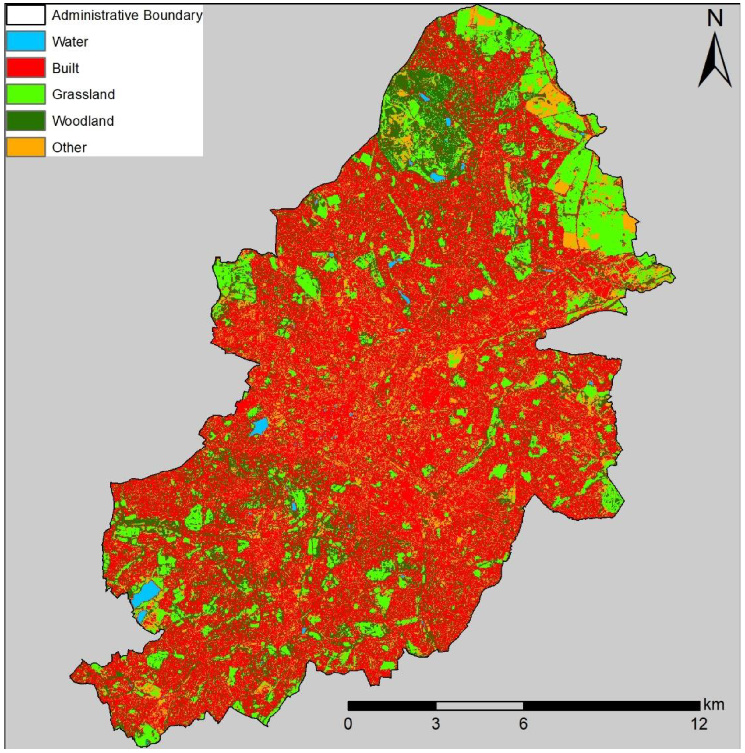
2.1. Datasets

To calculate the noise mitigation provided by urban trees, we used the following datasets. A 10 m resolution strategic noise modelling dataset for road noise, provided as a raster dataset by the Department for Food and Rural Affairs (Defra)—this dataset is hereafter referred to as the END noise data (created as requirement for Round 3 of the Environmental Noise Directive in 2017). The noise metric used is L_den (day, evening, night), calculated where Day is 7 a.m.–7 p.m. with a 0 dB penalty, Evening 7 p.m.–11 p.m. with a 5 dB penalty, and Night 11 p.m.–7 a.m. with a 10 dB penalty. It describes noise based on the energy equivalent sound level and is provided in units of A-weighted decibels (dBA), adjusted for the human perception of different frequencies. The road network is required for the spatial modelling of noise mitigation by trees and was obtained as a vector dataset from Ordnance Survey (OS) Open Roads. Residential buildings were derived from a polygon dataset from OS MasterMap. The population occupying residential buildings was a shapefile containing statistically disaggregated census data to building level, obtained from Defra. Data on urban tree cover was extracted from a land cover classification using Google Earth Engine, based on Sentinel-2 data, using a random forest classifier, described in the next section. All analyses were conducted at 10 m horizontal resolution, in OSGB36 National Grid coordinate reference system (Ordnance Survey Great Britain 1936), using R statistical software [22], using the r-packages ‘raster’ [23] and ‘gdistance’ [24].

We created a 10 m horizontal resolution raster land cover classification, based on Sentinel-2 data, using Google Earth Engine (Figure 1). The land cover dataset was created for the area within the Birmingham City Council administrative boundary plus an additional five-kilometre buffer. The training dataset consisted of 750 manually selected points; 150 for each of the five land cover classes (see

Table 1. Current land cover within the Birmingham City Council administrative boundary. The “other” class typically comprises bare, or seasonally bare (e.g., cropland) soil.

Land Cover	km2	Proportion
Water	1.5	0.5%
Built	147.6	55.1%
Grass	41.9	15.7%
Woodland	43.1	16.1%
Other	33.7	12.6%
Total	267.8	100%

for classes). Of the 750 training points, only 1 was misclassified, giving an overall accuracy of 0.998. Visual assessment of the two most important classes (woodland and grassland) against aerial imagery confirmed a high level of concordance. Such classification approaches may struggle to differentiate small areas (i.e., ≤100 m²) of any land cover type, including individual trees. However, individual trees provide a negligible level of noise mitigation, so potential omissions of single or small patches of trees are acceptable in the context of this study.

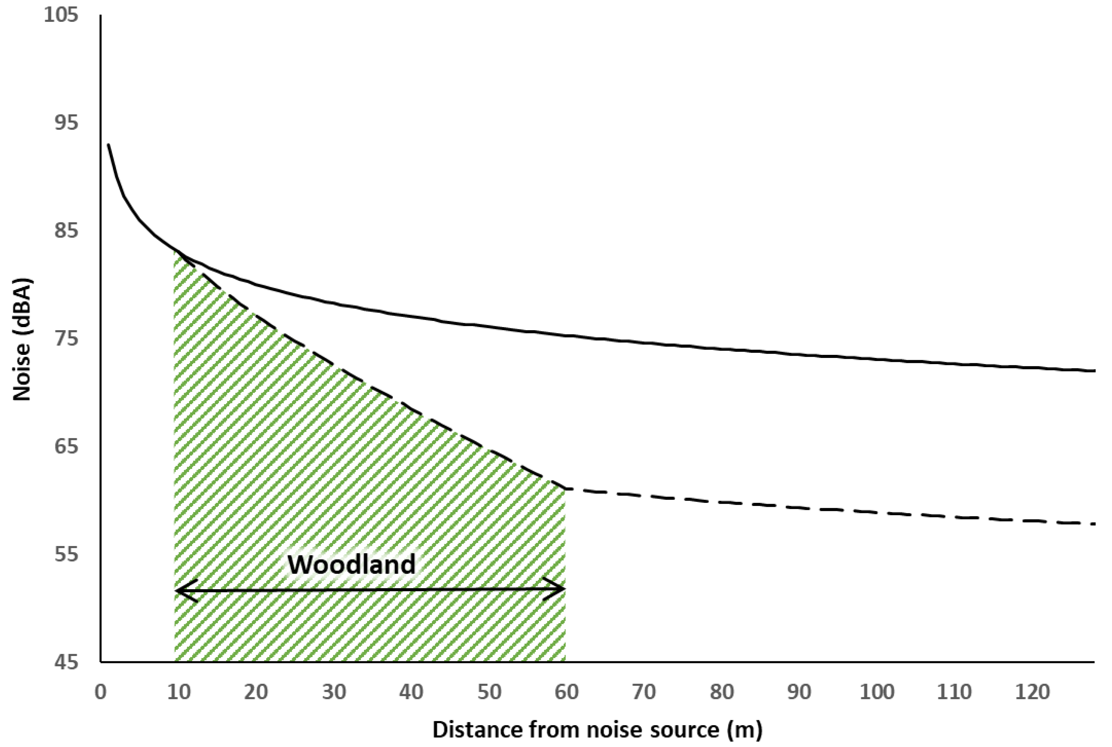
2.2. Calculating Noise Mitigation Provided by Trees

Using the END noise maps to guide the direction of travel, we measure for each grid cell, the minimum accumulated distance travelled from the noise sources, in this case roads. By then overlaying data representing woodland, we can measure how much of the distance travelled is through woodland. Knowing the distance travelled, and the proportion of this distance that is travelled through woodland, we can calculate for each cell the increase in noise attenuation, i.e., the difference between “no trees” and “with trees”. We do this by applying a function that represents established relationships between noise level and distance travelled through woodland (“insertion loss”, after van Renterghem [8]).

Mitigation calculations were undertaken in raster form, using the END noise maps as the structural template, i.e., 10 m horizontal resolution for the extent of the study area plus a 5 km buffer around it, to prevent edge effects/artefacts. As mentioned above, in order to map the noise mitigation provided by trees, we need to calculate two key parameters for each grid cell: (i) distance travelled from noise source, following the direction of noise in END noise map; (ii) the amount of that distance that is travelled through woodland. Once we know both of these figures, we can apply the Insertion Loss (IL) factor, per m of woodland, for each grid cell. This final figure will be the level of noise mitigation received from woodland. The IL value that we apply relates to the amount of attenuation due to trees observed by van Renterghem [8], which is 0.284 dBA per metre, calculated from data in van Renterghem [8] (illustrated schematically in Figure 2).

We use this value as a start-point to calculate the mitigation effects of trees. However, whilst van Renterghem [8] measures depth of tree stands using the stems (trunks) to delimit the patch, our data represent tree canopy, which will cover a greater area. Because of the nature of the data depicting woodland in our analysis (i.e., raster pixels, at 10 m horizontal resolution), in order to constitute a substantial barrier to noise, a patch of woodland may need to be 20–30 m depth (orthogonal to noise source), otherwise the noise could seep through the narrow points where neighboring raster cells meet only at the corners (consider a diagonal line of raster cells). Taking a 20–30 m depth (according to trunks of trees) patch of woodland, a likely canopy overhang of approximately 1–2 m at the edges (assuming it is established woodland) would constitute approximately 10–15% greater distance travelled through woodland when measured at canopy vs. measured at the trunks. Obviously, this proportion would diminish with larger patches of woodland, as the overhang represents proportionately less of the total distance. However, for most raster cells, the accumulated distance through woodland, from noise source, is <40 m for the current configuration of woodland. Therefore, in this analysis we have revised the 0.284 dBA m⁻¹ attenuation figure down to a slightly more conservative 0.25 dBA m⁻¹. In order to measure the two required distances (distance travelled and distance travelled through woodland), we exploit the concept of cost-distance across a 3-dimensional surface to model the propagation of sound across a landscape. We use the R-package ‘gdistance’ to construct transition matrices, containing data relating to the cost of traversing between adjacent raster cells (in 8 directions—also referred to as ‘queen’s move’ in chess), and to then calculate the minimum anisotropic accumulated cost surface from one or more origin points (cells corresponding to noise sources; roads). By adjusting the values in the transition matrix, for those cells corresponding with woodland (see Supplementary Materials for details of the adjustments and for flow diagram of modelling process), and calculating the minimum anisotropic accumulated cost surface for each version of the matrix, we can then calculate for each cell: distance travelled from noise source (m), and then the distance travelled through woodland, which allows us to apply the IL constant to calculate the amount of noise mitigation provided at the location of the raster cell.

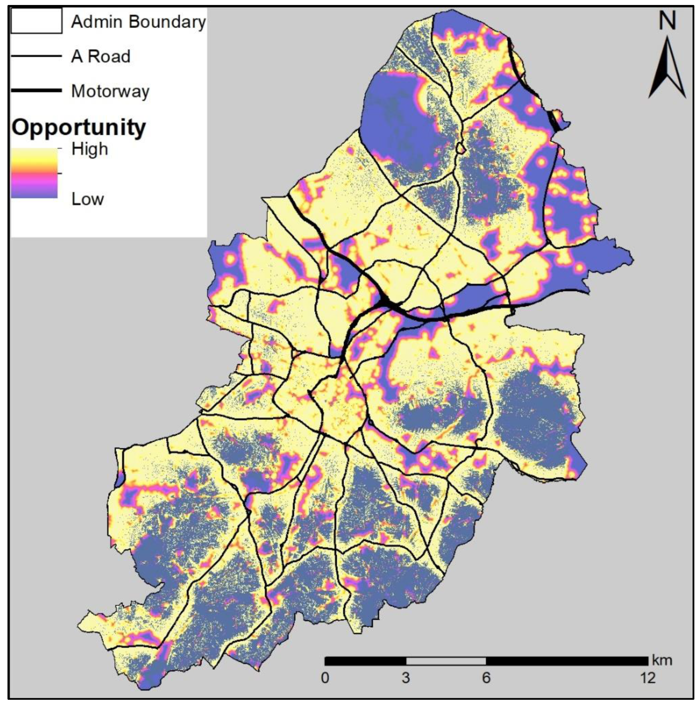
2.3. Opportunity Mapping

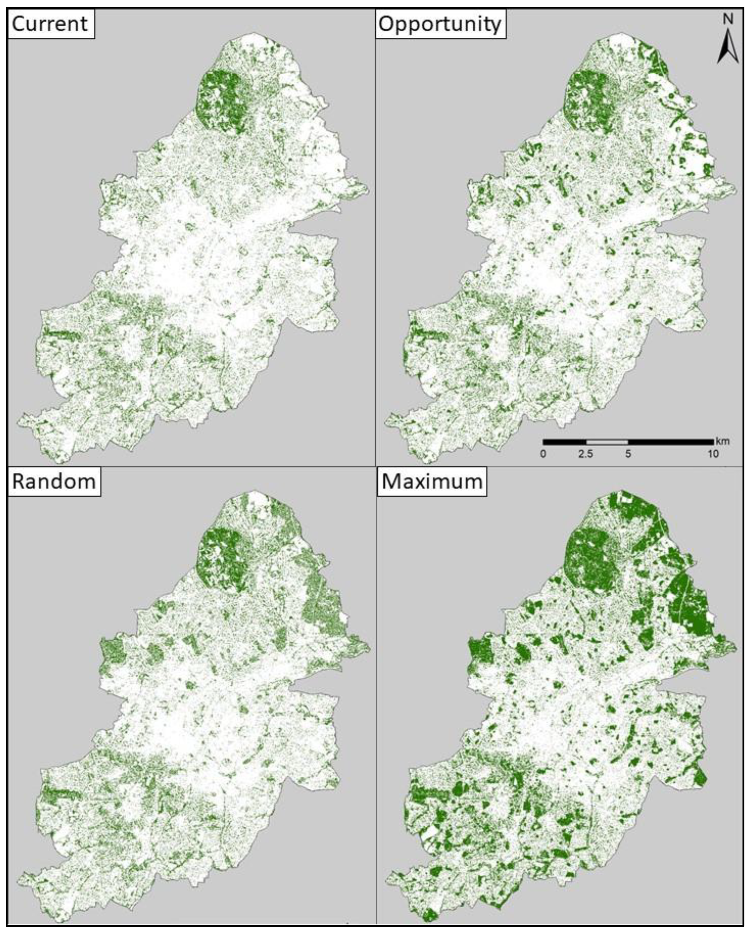
Opportunity mapping involves identifying locations that lie between noise sources and people (in this case, residential buildings), as these will be the best locations to position woodland for the purpose of noise mitigation (see Figure S2 in Supplementary Materials for flow diagram of opportunity modelling process). We updated the END noise map data to reflect the noise mitigation provided by the current woodland configuration. We then calculated the level of noise to which each residential building was exposed, by extracting values from the raster data to the building polygons, retaining the maximum value for each as a new attribute. Since economic valuation protocols typically disregard noise exposure below 50 dBA L_den, we selected and retained only those residential buildings with exposure levels of ≥50 dBA L_den. We then calculated a minimum anisotropic accumulated cost surface, using the END noise map as the surface and cells corresponding to the subset of the residential building polygons as the source points. For this calculation we effectively use the buildings as the source, by inverting the END noise map data (subtracting each value from the maximum value), so that the direction of travel would always be towards the roads. Once we had produced the accumulated cost raster, we inverted the values again (subtracting them from the maximum value), masked the raster, using the updated END noise map data to remove any regions where the noise levels were below 50 dBA L_den, and then converted to a percentage of the maximum value. This produced a raster with values ranging from 0 to 100, representing the proximity to residential buildings exposed to >50 dBA L_den, between these buildings and the noise sources.

2.4. Scenarios

In order to answer the three research questions set out at the end of the Introduction section, we obtain mapped estimates of noise levels for a total of five scenarios (see

Table 2. Names and descriptions of the woodland configuration scenarios, with the proportional coverage of woodland in parentheses.

Name	Description	Coverage
No Woodland	No trees	0%
Current	Current woodland configuration	16.1%
Random	Additional woodland area selected randomly from within grassland areas ≥ 50 dB(A)	20%
Opportunity	Additional woodland area selected from grassland using opportunity map scores	20%
Maximum	All grassland replaced with woodland	31.8%

), each representing differing quantities and/or configurations of woodland. In constructing these scenarios, where it was necessary to add woodland beyond the current configuration, we used grassland as the candidate land cover type for conversion. We did this because grassland is the most likely land cover type to be feasible to replace with woodland in cities.

To calculate the mitigation provided by any particular configuration of woodland in Birmingham, it was necessary to have a ‘no woodland’ scenario as our baseline, so that we could subtract the mapped noise levels for a particular configuration against this reference. Since the END noise mapping approach does not account for the mitigating effect of trees, this constitutes the noise levels for a no woodland scenario. The first wooded scenario is ‘current’ woodland, where woodland covered 16.1% of the administrative region.

To calculate the maximum possible provision of noise mitigation by woodland, we needed to calculate noise levels for a ‘maximum’ woodland scenario, where all grassland within Birmingham city administrative region was replaced with woodland. In total, woodland in this scenario covered 31.8% of the administrative region.

To test the effectiveness of our opportunity mapping approach, we constructed an ‘opportunity’ scenario, where we used our opportunity mapping scores to allocate which grassland grid-cells were to be replaced by woodland. We selected grassland grid-cells corresponding with the top opportunity scores, until the total area of woodland constituted 20% of the Birmingham City administrative region—a figure that aligns closely with the near-term policy ambitions of the City, although longer-term ambitions are for 25–30% (see [25]). We then constructed a ‘random’ scenario with the same total area of woodland, against which to compare the opportunity mapping approach. In this scenario, the grassland grid-cells were selected randomly from within areas exposed to noise levels ≥ 50 dBA L_den, until the total area of woodland constituted 20% of the administrative region.

2.5. Quantifying Exposure and Economic Value of Mitigation for Scenarios

Economic valuation followed methods from the ‘handbook on the external costs of transport’ [26], henceforth referred to as ‘the handbook’. Health and annoyance costs in the handbook are calculated independently, as they use different approaches. Annoyance costs are calculated using a Willingness To Pay (WTP) approach—respondents are asked how much they would be willing to pay for specified reductions in noise. Health costs are calculated using an environmental burden of disease method (for details, see [27]). For both health and annoyance, the costs increase with the level of exposure. Van Essen et al. [26] provide costs, per decibel (dependent upon how high the noise level is), per person, per year, for annoyance and health (see

Table 3. Environmental price of traffic noise for the EU28 (EUR 2016/dB/person/year)—road transport section of Table 33, from [26].

Lden (db(A))	Road Transport
	Annoyance	Health	Total
50–54	14	3	17
55–59	28	3	31
60–64	28	6	34
65–69	54	9	63
70–74	54	13	67
≥75	54	18	72

, below).

For each scenario, we quantified noise exposure at individual residential buildings using the approach described in the opportunity mapping section, giving noise exposure figures for each building under each of the five scenarios. Using these figures, we calculated the costs associated with noise exposure for each of our five scenarios. By subtracting the costs of noise in our four scenarios that include woodland from the ‘No Woodland’ scenario costs, we calculated the value of the mitigation in each woodland scenario. As the figures in the handbook are in 2016 Euros, we converted the final figures to GBP and corrected for inflation to give 2019 prices.

3. Results

The opportunity mapping process (see Figure 3) identified the noisy areas between roads and residential buildings. As expected, the greatest opportunity lies alongside the noisiest roads, but only where there are residential buildings that would benefit from noise mitigation. The more distributed areas of high opportunity in the centre of the map take into account noise generated by many smaller roads not illustrated in this figure.

The maps of woodland allocation under each scenario are shown in Figure 4. The maximum scenario, where all grassland is converted to woodland, highlights the extent of the potential woodland candidate sites. The woodland in the random scenario broadly covers the same areas, but in a much sparser fashion. The more focused distribution of woodland in the opportunity scenario map is apparent when compared with the random scenario map, particularly in the north-eastern region of the city, along the administrative boundary. These aggregations of new woodland are around roads and residential buildings.

Noise mitigation was calculated for the whole of the Birmingham City Council area, illustrated using a zoomed-in region in Figure 5 to show the detail. The areas receiving the most mitigation are shaded in lighter colours in the two lower panels of Figure 5. The noise mitigation provided by woodland is greatest in areas shielded by trees, with the highest values in areas behind deeper stands of woodland. The level of mitigation in these regions then diminishes with distance from the woodland, moving away from the noise source, due to a flanking effect of noise around obstacles. A number of residential buildings can be seen to be receiving mitigation benefit from the woodland in the zoomed-in example of the current woodland configuration.

In the Current scenario, existing woodland in Birmingham provides a mitigation benefit to just over 52,000 residential buildings (

Table 4. The number of Buildings, People and Dwellings (defined as self-contained units of accommodation) exposed to >50 dBA L_den, which receive mitigation from woodland, calculated by difference from the ‘No Woodland’ scenario.

Scenario	Buildings	Population	Dwellings
Current	52,066	177,446	74,993
Random	56,457	196,770	83,732
Opportunity	61,157	216,181	92,372
Maximum	62,478	221,151	94,755

). Comparing the results from each of the different woodland scenarios, there are substantial differences in the number of dwellings that receive mitigation (Table 4). As expected, the Current scenario provides mitigation to the lowest number of dwellings, and the Maximum scenario provides mitigation to the greatest number of dwellings. However, for the two scenarios with an intermediate area of added woodland, Random and Opportunity, there is a substantial difference in the number of dwellings receiving mitigation, with woodland in the Opportunity scenario providing mitigation to substantially more dwellings than that of the Random scenario, and very close to the number of dwellings mitigated in the Maximum scenario. The number of people per dwelling is relatively consistent, averaging 2.34 ± 0.01.

The differences in the number of dwellings receiving mitigation translate into analogous differences in the economic value of mitigation for the Opportunity scenario, which in both cases is 97% of that achieved in the Maximum scenario. However, the Random scenario provides both less benefit, and to fewer dwellings, compared with the Maximum scenario (72% and 88%, respectively).

The value of noise mitigation provided by the current configuration of woodland in Birmingham is GBP 3.83 million, which is approximately 6% of the total cost (annoyance and health combined) of road traffic noise for the city under the No Woodland scenario. Converting all grassland to woodland, which constitutes an almost doubling of woodland cover, achieves mitigation to the value of GBP 6.29 million. However, the addition of just 3.9% woodland cover in the Opportunity scenario leads to a total mitigation value of GBP 6.09 million.

Looking at the efficiency of woodland at mitigating noise in each of the scenarios (

Table 5. For each scenario, the % woodland cover, the costs of noise exposure, the value of noise mitigation provided by woodland and average value of mitigation per hectare of woodland (GBP ₂₀₁₉). Mitigation value is calculated using the total costs, by subtracting the costs for each scenario from the costs for the ‘No woodland’ scenario.

Scenario	Woodland Cover (ha)	Annoyance Cost (Millions)	Health Cost (Millions)	Total Cost (Millions)	Mitigation Value (Millions)	Average Mitigation Value ha−1
No Woodland	-	GBP 56.76	GBP 9.98	GBP 66.74	-	-
Current	4312	GBP 53.52	GBP 9.40	GBP 62.91	GBP 3.83	GBP 887
Random	5356	GBP 52.89	GBP 9.29	GBP 62.18	GBP 4.56	GBP 851
Opportunity	5356	GBP 51.60	GBP 9.05	GBP 60.65	GBP 6.09	GBP 1136
Maximum	8516	GBP 51.42	GBP 9.02	GBP 60.45	GBP 6.29	GBP 738

), the Current scenario provides mitigation to the value of GBP 887 per hectare, while the Random and Maximum scenarios provide less than this, the latter being the least efficient. Of the four scenarios, the Opportunity scenario is substantially more effective per unit area, at GBP 1136 per hectare—one-third more than the Random scenario.

4. Discussion

Our results show that more than 177,000 people in Birmingham city currently benefit from the noise mitigation provided to their homes by woodland, worth an estimated GBP 3.83 million per annum. The comparison of the scenarios of woodland placement in our analyses shows that the opportunity mapping performs very well as a means for targeting new woodland placement to tackle traffic noise, the Opportunity scenario providing 97% of the mitigation provided by the Maximum scenario, with only a quarter of the added woodland area (1044 ha compared to 4204 ha).

The methods presented here provide a robust new way of mapping the mitigating effect of woodland on road traffic noise at a large scale: whole city, regional, or even national. Compared with the other methods that are commonly used to quantify this noise mitigation ecosystem service (see Section 1), our new approach better accounts for the critical factors of position of people (i.e., residential buildings), relative to noise sources and relative to woodland. This allows the approach to identify mitigation in the correct areas, i.e., where woodland would be shielding from the propagation of sound. Taking account of the beneficiaries and the spatial location of service provision is now recognised as essential for many ecosystem services [28,29,30]. Moreover, this mitigation is proportional to the depth of the woodland, in the direction of the sound, which means that the model goes further than a simple binary mitigation/no mitigation output (e.g., [20]). In turn, this allows us to quantify changes in the levels of noise exposure of people (here, residential buildings), which can be valued (monetary) or quantified in terms of health impacts (e.g., disability-adjusted life years).

The land cover classification that we use in this study slightly underestimates the actual tree cover of Birmingham city compared with the estimate given in the Birmingham Urban Forest Master Plan [31] for 2019: 16.1% here, compared with 18.6% from Bluesky National Tree Map™. The latter is a commercial product and was not available for this study. Furthermore, it is a trees only data layer and for the creation of our potential woodland scenarios (i.e., Random, Opportunity and Maximum scenarios), we also needed to identify potential candidate locations for new woodland (i.e., grassland areas), which meant we needed a full land cover dataset. Nonetheless, the presented methods for quantifying noise mitigation by woodland can in principle be applied using any woodland or tree canopy spatial dataset.

Our noise model uses the insertion loss (IL) coefficient from van Renterghem [8], based on a uniform planting configuration and uniform tree trunk diameter. However, the planting configuration and trunk size and type of trees being planted can all influence the IL achieved [32,33]. In theory, these factors could also be incorporated into the noise model. This could be particularly useful when calculating overall cost benefits of planting schemes, considering the best size of trees to plant in order to maximise the ES benefits over longer time periods (see [34] for an example of such a discussion).

The economic valuation approach is based on the number of beneficiaries multiplied by their change in exposure to noise. Therefore, the final valuation could be influenced by the accumulation of many instances of small changes in exposure (i.e., very low levels of mitigation). The ability of the human ear to detect small changes in the noise level of a pure tone varies substantially, depending on the initial noise level. However, its ability to detect changes in the level of broadband noise, such as traffic noise, tends to be relatively consistent above 30 dB, able to detect changes of around 0.5 dB [35]. When we checked each of our scenarios, the proportion of the mitigation provided by woodland that was <0.5 dBA was only 10–13% of the total mitigation value; therefore, these low values make only a small contribution to the overall calculation of economic value.

The presented noise modelling method is reliant on existing spatial information on noise levels: the END data. Due to the nature of these data (i.e., the resolution and extent of modelled area as well as the annually averaged metrics), they are not validated against actual noise level measurements, as the collection of a suitable validation dataset would be prohibitively expensive and time-consuming. The paucity of such a validation dataset also means that we cannot fully validate our model outputs. Nonetheless, spatially, our mitigation maps indicate that mitigation is occurring in the expected locations, and by using a conservative approach (i.e., moderated IL coefficient), we minimise the likelihood that our model overstates the level of mitigation provided.

Further work is necessary in order to create a version of the model that can be used in locations where END data are not available (i.e., cities, regions, countries for which there are no noise maps). Some indication of noise level is needed in order to calculate impacts, as the calculations are dependent upon the reference noise level (i.e., before accounting for mitigation) as well as the magnitude of the change. Software for modelling traffic noise is freely available (e.g., see [36]); however, a major impediment to creating detailed noise maps is the lack of freely available traffic data.

The opportunity mapping presented here allows a dynamic approach to identifying optimal locations for a particular service, which is still relatively uncommon in ES modelling. In practice, this means that placement of new trees can be targeted to ensure improved effectiveness at mitigating noise. The opportunity mapping could be further refined or customised by the addition of other data, to target particular areas of the city, or particular demographics within the population that are more vulnerable to the effects of noise pollution—e.g., children, the elderly and the chronically ill, who may have a high sensitivity and/or low resilience [37]. When adding new woodland in a scenario, each addition will change the resulting opportunity scores. Ideally, the allocation of new woodland should be conducted in an iterative process, where the residential buildings exposed to the greatest noise levels are always prioritised above those that are exposed to lower noise levels, or where feasibility/cost of implementation are used to weight allocation decisions. In this study, we use grassland as a universal candidate land cover for replacement by woodland, however this does not take into account the ownership of this land, or the actual feasibility for it to be replaced. Some of the land will inevitably be private gardens, football pitches, sports fields, golf courses, and so on. Therefore, there is scope to use additional datasets to constrain the opportunity mapping process so that only sites that can be converted are included in the scoring. For example, distinguishing the mitigation potential of land in public ownership and in private ownership might help design specific funding mechanisms to bring about the desired changes. Green spaces in private ownership also provide ES, and should be included in ES mapping and in the process of urban planning (e.g., see [38,39]). Another important factor that could be integrated into opportunity mapping is that of dis-benefits, i.e., negative impacts resulting from the placement of the new woodland. Such dis-benefits can range from the production of biogenic volatile organic compounds (BVOCs) to the shading of buildings, or the blocking of views. As with the benefits of new woodland, the dis-benefits tend to be highly context-dependent. For instance, shading of buildings that suffer from excessive heat in the summer months might be seen as a benefit, but shading of buildings that have no such concerns might actually require additional expenditure on internal lighting that would otherwise not be necessary.

Noise mitigation is of course not the only ES that urban woodland provides. The removal of particulate air pollution is another good example of an urban woodland ES that is highly context-dependent, with greater service provided by trees in areas with greater atmospheric concentrations of particulates [40,41]. Indeed, there may well be some synergies amongst the numerous ES provided by urban woodland and more generally, urban green space (UGS). However, some ES might require substantially different spatial configurations of UGS in order to provide optimal efficiency (e.g., placement of woodland for flood mitigation will be upstream, perhaps miles away from busy roads) [42]. The overall optimal placement of woodland then requires the evaluation of multiple spatial planning scenarios [43], and the opportunity mapping scores presented here help to design the scenarios that are optimal for noise mitigation.

5. Conclusions

Robust ES models and opportunity mapping can serve as important inputs for decision support tools. Whilst the planning of tree planting locations in a city is likely to have a number of constraints/aims, noise mitigation is often not currently a consideration, perhaps because of a lack of relevant information concerning the magnitude of the noise pollution problem and the potential benefits of effective placement of trees to provide mitigation.

The combination of a spatially explicit model and sophisticated opportunity mapping allows a highly targeted approach to identify optimum locations for tree planting for noise mitigation. In this study, we show that you can achieve close to a maximum service with less than a quarter of the additional woodland needed to achieve the maximum. Such a targeted approach can also provide cost savings, since the efficiency per unit area of woodland was increased by over 30% compared with an untargeted planting scenario.

This has important implications for the design and implementation of urban tree planting for noise mitigation, and these methods can be adapted for other ES allowing consideration of multiple service outcomes. Ultimately, this approach can help city officials and planners to better design interventions based on green and blue infrastructure to achieve improved benefits for city residents.

References

1. Bolund, P.; Hunhammar, S. Ecosystem services in urban areas. Ecol. Econ. 1999, 29, 293–301. [Google Scholar] [CrossRef]
2. Hänninen, O.; Knol, A.B.; Jantunen, M.; Lim, T.A.; Conrad, A.; Rappolder, M.; Carrer, P.; Fanetti, A.-C.; Kim, R.; Buekers, J.; et al. Environmental burden of disease in Europe: Assessing nine risk factors in six countries. Environ. Health Perspect. 2014, 122, 439–446. [Google Scholar] [CrossRef] [PubMed] [Green Version]
3. Hammer, M.S.; Swinburn, T.K.; Neitzel, R.L. Environmental noise pollution in the United States: Developing an effective public health response. Environ. Health Perspect. 2014, 122, 115–119. [Google Scholar] [CrossRef] [PubMed] [Green Version]
4. Münzel, T.; Gori, T.; Babisch, W.; Basner, M. Cardiovascular effects of environmental noise exposure. Eur. Heart J. 2014, 35, 829–836. [Google Scholar] [CrossRef] [PubMed] [Green Version]
5. Münzel, T.; Sørensen, M.; Gori, T.; Schmidt, F.P.; Rao, X.; Brook, F.R.; Rajagopalan, S.; Chen, L.C.; Brook, R.D. Environmental stressors and cardio-metabolic disease: Part II–mechanistic insights. Eur. Heart J. 2017, 38, 557–564. [Google Scholar] [CrossRef] [PubMed]
6. Hammer, M.S.; Fan, Y.; Hammer, S.S.; Swinburn, T.K.; Weber, M.; Weinhold, D.; Neitzel, R.L. Applying a novel environmental health framework theory (I-ACT) to noise pollution policies in the United States, United Kingdom, and the Netherlands. J. Environ. Plan. Manag. 2018, 61, 2111–2132. [Google Scholar] [CrossRef]
7. Hurtley, C. (Ed.) Night Noise Guidelines for Europe; WHO Regional Office Europe: Copenhagen, Denmark, 2009. [Google Scholar]
8. van Renterghem, T. Guidelines for optimizing road traffic noise shielding by non-deep tree belts. Ecol. Eng. 2014, 69, 276–286. [Google Scholar] [CrossRef] [Green Version]
9. HOSANNA. Novel Solutions for Quieter and Greener Cities; EU FP7: Bandhagen, Sweden, 2013. [Google Scholar]
10. Tang, S.H.; Ong, P.P.; Woon, H.S. Monte Carlo simulation of sound propagation through leafy foliage using experimentally obtained leaf resonance parameters. J. Acoust. Soc. Am. 1986, 80, 1740–1744. [Google Scholar] [CrossRef]
11. van Renterghem, T.; Botteldooren, D.; Verheyen, K. Road traffic noise shielding by vegetation belts of limited depth. J. Sound Vib. 2012, 331, 2404–2425. [Google Scholar] [CrossRef] [Green Version]
12. Eigenbrod, F.; Armsworth, P.R.; Anderson, B.J.; Heinemeyer, A.; Gillings, S.; Roy, D.B.; Thomas, C.D.; Gaston, K.J. The impact of proxy-based methods on mapping the distribution of ecosystem services. J. Appl. Ecol. 2010, 47, 377–385. [Google Scholar] [CrossRef]
13. Thomas, A.; Masante, D.; Jackson, B.; Cosby, B.; Emmett, B.; Jones, L. Fragmentation and thresholds in hydrological flow-based ecosystem services. Ecol. Appl. 2020, 30, e02046. [Google Scholar] [CrossRef] [PubMed]
14. Villa, F.; Bagstad, K.J.; Voigt, B.; Johnson, G.W.; Portela, R.; Honzák, M.; Batker, D. A methodology for adaptable and robust ecosystem services assessment. PLoS ONE 2014, 9, e91001. [Google Scholar] [CrossRef] [PubMed]
15. Andersson-Sköld, Y.; Klingberg, J.; Gunnarsson, B.; Cullinane, K.; Gustafsson, I.; Hedblom, M.; Knez, I.; Lindberg, F.; Sang, Å.O.; Pleijel, H.; et al. A framework for assessing urban greenery’s effects and valuing its ecosystem services. J. Environ. Manag. 2018, 205, 274–285. [Google Scholar] [CrossRef] [PubMed]
16. Gratani, L.; Varone, L. Carbon sequestration and noise attenuation provided by hedges in Rome: The contribution of hedge traits in decreasing pollution levels. Atmos. Pollut. Res. 2013, 4, 315–322. [Google Scholar] [CrossRef] [Green Version]
17. Geneletti, D.; Cortinovis, C.; Zardo, L.; Esmail, B.A. Towards equity in the distribution of ecosystem services in cities. In Planning for Ecosystem Services in Cities; Springer: Cham, Switzerland, 2020; pp. 57–66. [Google Scholar]
18. Derkzen, M.L.; van Teeffelen, A.J.; Verburg, P.H. Quantifying urban ecosystem services based on high-resolution data of urban green space: An assessment for Rotterdam, the Netherlands. J. Appl. Ecol. 2015, 52, 1020–1032. [Google Scholar] [CrossRef]
19. Ramyar, R. Social–ecological mapping of urban landscapes: Challenges and perspectives on ecosystem services in Mashhad, Iran. Habitat Int. 2019, 92, 102043. [Google Scholar] [CrossRef]
20. Cortinovis, C.; Geneletti, D. A performance-based planning approach integrating supply and demand of urban ecosystem services. Landsc. Urban Plan. 2020, 201, 103842. [Google Scholar] [CrossRef]
21. Geneletti, D. Reasons and options for integrating ecosystem services in strategic environmental assessment of spatial planning. Int. J. Biodivers. Sci. Ecosyst. Serv. Manag. 2011, 7, 143–149. [Google Scholar] [CrossRef] [Green Version]
22. R Core Team. R: A Language and Environment for Statistical Computing; R Foundation for Statistical Computing: Vienna, Austria, 2016; Available online: https://www.R-project.org/ (accessed on 1 February 2018).
23. Hijmans, R.J.; van Etten, J. Raster: Geographic Data Analysis and Modeling. R Package Version 2.5–8. 2016. Available online: https://CRAN.R-project.org/package=raster (accessed on 1 February 2018).
24. van Etten, J. R package gdistance: Distances and routes on geographical grids. J. Stat. Softw. 2017, 76, 1–21. [Google Scholar] [CrossRef] [Green Version]
25. BCC. Birmingham City Council—Birmingham Tree Policy Report. 2018. Available online: https://www.birmingham.gov.uk/downloads/file/16847/ebd23_bcc_birmingham_tree_policy_report_feb_2018 (accessed on 6 February 2018).
26. van Essen, H.; van Wijngaarden, L.; Schroten, A.; de Bruyn, S.; Sutter, D.; Bieler, C.; Beyrouty, K.E. Handbook on the External Costs of Transport; Version 1.1; European Commission; Luxembourg Publications Office of the European Union: Luxembourg, 2019. [Google Scholar]
27. DEFRA. Noise Pollution: Economic Analysis. Department for Environment, Food & Rural Affairs, UK Government. 2014. Available online: https://www.gov.uk/guidance/noise-pollution-economic-analysis (accessed on 1 February 2018).
28. Holt, A.R.; Mears, M.; Maltby, L.; Warren, P. Understanding spatial patterns in the production of multiple urban ecosystem services. Ecosyst. Serv. 2015, 16, 33–46. [Google Scholar] [CrossRef] [Green Version]
29. Cimburova, Z.; Pont, M.B. Location matters. A systematic review of spatial contextual factors mediating ecosystem services of urban trees. Ecosyst. Serv. 2021, 50, 101296. [Google Scholar] [CrossRef]
30. Jones, L.; Boeri, M.; Christie, M.; Durance, I.; Evans, K.L.; Fletcher, D.; Harrison, L.; Jorgensen, A.; Masante, D.; McGinlay, J.; et al. Can we model cultural ecosystem services, and are we measuring the right things? People Nat. 2022, 4, 166–179. [Google Scholar] [CrossRef]
31. Rogers, K.; van den Bosch, C.K.; Vaughan-Johncey, C. An Urban Forest Master Plan for Birmingham 2021–2051. Executive Report. 2021. Available online: https://secureservercdn.net/160.153.138.71/d9o.bd8.myftpupload.com/wp-content/uploads/2021/11/BUFMPExecReport-Final-Nov-2021-v1.pdf (accessed on 19 November 2021).
32. van Renterghem, T.; Attenborough, K.; Jean, P. Designing vegetation and tree belts along roads. In Environmental Methods for Transport Noise Reduction; Nilsson, M., Bengtsson, J., Klæboe, R., Eds.; CRC Press: Boca Raton, FL, USA, 2015. [Google Scholar]
33. Ow, L.F.; Ghosh, S. Urban cities and road traffic noise: Reduction through vegetation. Appl. Acoust. 2017, 120, 15–20. [Google Scholar] [CrossRef]
34. Walters, M.; Sinnett, D. Achieving tree canopy cover targets: A case study of Bristol, UK. Urban For. Urban Green. 2021, 65, 127296. [Google Scholar] [CrossRef]
35. Fastl, H.; Zwicker, E. Just-Noticeable Sound Changes. In Psychoacoustics; Springer: Berlin/Heidelberg, Germany, 2007. [Google Scholar] [CrossRef]
36. Gulliver, J.; Morley, D.; Vienneau, D.; Fabbri, F.; Bell, M.; Goodman, P.; Beevers, S.; Dajnak, D.; Kelly, F.J.; Fecht, D. Development of an open-source road traffic noise model for exposure assessment. Environ. Model. Softw. 2015, 74, 183–193. [Google Scholar] [CrossRef] [Green Version]
37. Syrbe, R.U.; Walz, U. Spatial indicators for the assessment of ecosystem services: Providing, benefiting and connecting areas and landscape metrics. Ecol. Indic. 2012, 21, 80–88. [Google Scholar] [CrossRef]
38. Pristeri, G.; Peroni, F.; Pappalardo, S.E.; Codato, D.; Masi, A.; De Marchi, M. Whose Urban Green? Mapping and Classifying Public and Private Green Spaces in Padua for Spatial Planning Policies. ISPRS Int. J. Geo-Inf. 2021, 10, 538. [Google Scholar] [CrossRef]
39. Dewaelheyns, V.; Rogge, E.; Gulinck, H. Putting domestic gardens on the agenda using empirical spatial data: The case of Flanders. Appl. Geogr. 2014, 50, 132–143. [Google Scholar] [CrossRef]
40. Nemitz, E.; Vieno, M.; Carnell, E.; Fitch, A.; Steadman, C.; Cryle, P.; Holland, M.; Morton, R.D.; Hall, J.; Mills, G.; et al. Potential and limitation of air pollution mitigation by vegetation and uncertainties of deposition-based evaluations. Philos. Trans. R. Soc. A 2020, 378, 20190320. [Google Scholar] [CrossRef] [PubMed]
41. Fletcher, D.H.; Likongwe, P.J.; Chiotha, S.S.; Nduwayezu, G.; Mallick, D.; Md, N.U.; Rahman, A.; Golovátina-Mora, P.; Lotero, L.; Bricker, S.; et al. Using demand mapping to assess the benefits of urban green and blue space in cities from four continents. Sci. Total Environ. 2021, 785, 147238. [Google Scholar] [CrossRef]
42. Hutchins, M.G.; Fletcher, D.; Hagen-Zanker, A.; Jia, H.; Jones, L.; Li, H.; Loiselle, S.; Miller, J.; Reis, S.; Seifert-Dähnn, I.; et al. Why scale is vital to plan optimal Nature-Based Solutions for resilient cities. Environ. Res. Lett. 2021, 16, 044008. [Google Scholar] [CrossRef]
43. Madureira, H.; Andresen, T. Planning for multifunctional urban green infrastructures: Promises and challenges. Urban Des. Int. 2014, 19, 38–49. [Google Scholar] [CrossRef]
Figure 1. Land cover classification created in Google Earth Engine, using cloud-free Sentinel-2 Surface Reflectance data from 1 January 2019–1 January 2020.
Sustainability 14 07079 g001
Figure 2. An example of how noise level changes over open ground (solid line—no mitigation), and through woodland stretching from 10 m–60 m (dashed line—mitigated by trees). Noise decline in open air is 3 dBA per doubling of distance for a linear noise source. Note that the rate of attenuation of noise is greater than noise in open air, by an additional linear rate of 2.84 dBA m−1 only whilst travelling through woodland.
Sustainability 14 07079 g002
Figure 3. Opportunity map, for full extent of Birmingham City Council administrative region.
Sustainability 14 07079 g003
Figure 4. The woodland scenarios for which mitigation was valued. Clockwise from top left: current woodland configuration; targeted allocation of woodland, using opportunity mapping scores; random allocation of woodland; maximum woodland, where all grassland is converted to woodland.
Sustainability 14 07079 g004
Figure 5. Four panels, clockwise from top left are: full extent of Birmingham administrative region plus five km buffer, with END noise map, showing the zoomed region in the following three panels; END noise map data and woodland; noise mitigation and woodland; noise mitigation, woodland and residential buildings.
Sustainability 14 07079 g005