Article

Location Optimization of Fresh Agricultural Products Cold Chain Distribution Center under Carbon Emission Constraints

1
College of Economics and Management, Qingdao Agricultural University, Qingdao 266109, China
2
College of Humanities and Social Sciences, Qingdao Agricultural University, Qingdao 266109, China
*
Authors to whom correspondence should be addressed.
Sustainability 2022, 14(11), 6726; https://doi.org/10.3390/su14116726
Submission received: 12 May 2022 / Revised: 27 May 2022 / Accepted: 27 May 2022 / Published: 31 May 2022

Abstract

:
This paper seeks to effectively realize energy saving and emission reduction in the process of location for fresh agricultural cold chain logistics. It is based on the traditional location for distribution center optimized for both freshness and carbon emissions. A bi-objective function location model was constructed to minimize the total cost and carbon emission and a two-stage heuristic algorithm was designed to solve the model. According to analyzing the location case of Y enterprise in Zhejiang Province, the THA had an average total cost optimization rate of 7.70% and an average carbon emission optimization rate of 10.23% compared to the WOA, while it had a rate of 12.77% and 14.12%, respectively, compared to the PSO. When the unit carbon emission cost increased from 0.02 dollar/kg to 0.06 dollar/kg, the comprehensive carbon emission cost increased by 42.07% and the total cost increased by 3.05%. Therefore, logistics enterprises can achieve the reduction of logistics costs and sustainable development through reasonable location for fresh agricultural products cold chain distribution centers.

1. Introduction

As people’s living standards improve, the demand for the cold chain for fresh agricultural products is on the rise, and the quality requirements of such products are getting more stringent [1,2,3]. Since fresh agricultural products are vulnerable and need to be delivered on time, different procedures of logistics are independent of each other in the traditional cold chain system, so it is difficult to transport these goods under a stable temperature during the whole transit [4,5]. Meanwhile, the unreasonable use of devices such as cold storage, refrigerated vehicles, and automated temperature control consumes a lot of energy, causes large carbon emissions, and harms the environment [6,7]. As the concept of sustainable development prevails, the domestic carbon trading market has been initially launched, and the government-led policies of energy conservation and emission reduction have been gradually transformed into a market-oriented state [8], in which market regulation is made full use of to promote the green emission reduction of enterprises.
In this context, the optimal location decision of the cold chain distribution center of fresh agricultural products can promote the reasonable planning and unified scheduling of the logistics system of the cold chain distribution center. While ensuring the quality of fresh agricultural products, which can effectively improve the utilization rate of cold chain equipment, reduce the cost of carbon emissions, and promote the sustainable development of the whole society [9,10,11].

2. Literature Review

2.1. Carbon Emissions from Cold Chain Logistics

With the deepening of the concept of sustainable development, scholars have conducted active research on how to reduce carbon emissions while ensuring the development of cold chain logistics. Early literature studies mainly used carbon footprint to optimize the configuration of the cold chain supply chain. For example, Tian [12] first proposed the carbon footprint of Xinjiang grape cold chain logistics, and used the single-stage supply chain profit model to conduct research and analysis; Benjaafar et al. [13] applied carbon footprint to the cold chain. In the structural analysis of the supply chain, optimization measures are proposed based on the carbon footprint of the milk supply chain. Although the research on the optimal configuration of the supply chain based on carbon footprint expands the theoretical connotation of carbon emissions in cold chain logistics, it is difficult for logistics companies to evaluate the specific carbon emissions in cold chain operations. In recent years, more and more scholars have analyzed and optimized cold chain logistics activities through carbon emission constraints. For example, Pan et al. [14] introduced carbon emission constraints into the cold chain logistics distribution process and transformed them into corresponding economic indicators. The structure considers carbon emissions and a cost-based quantitative model of cold chain logistics distribution path optimization. Li [15] considered the comprehensive cost of carbon, optimized the inventory and distribution process of the fresh supply chain warehouse, and established a two-level inventory-path optimization model with a time window. However, at present, there are relatively few studies that consider carbon emission factors in the location selection of cold chain logistics distribution centers. The location of distribution centers will directly affect vehicle routing and inventory allocation, and further, affect the dynamic carbon emissions in transportation and static carbon in warehousing. emission.

2.2. Location for Logistics Distribution Centers

The theoretical study of the location problem of logistics distribution centers (LDC) originated from Weber’s theory [16] in the early 20th century and was further extended by the P-median model proposed by Hakimi [17]. The location selection for logistics distribution centers is a typical NP-hard problem with a lot of complex constraints and non-smooth characteristics [18]. After decades of research and development, the solution to this type of problem can be divided into qualitative and quantitative location models. Qualitative models are mainly based on the construction of target evaluation systems for performance evaluation and ranking, such as the analytic hierarchy process [19], fuzzy evaluation method [20], grey relational degree method [21], etc. Qualitative models are beneficial to deal with uncertain influencing factors, and the evaluation results are rich in information, but the judgment level is more complicated, and it is difficult to meet the requirements of standardization and consistency. Quantitative models mainly calculate the location of the logistics distribution center through quantifiable indicators and are mainly divided into accurate solution methods and heuristic algorithms. The accurate algorithms for solving LDC are mainly based on the centroid method [22], linear programming method [23], Baumol–Wolfe model [24], etc. These algorithms can solve the optimal solution of the problem, but at the cost of time and space complexity in exchange for the quality of the understanding, they cannot be used to meet the needs of actually solving large-scale problems. The application of heuristic algorithms to solve LDC originated from the first use of a heuristic algorithm by Steven et al. to solve the logistics distribution center location problem considering inventory factors [25]. Heuristic algorithms mainly based on genetic algorithm [26], ant colony algorithm [27], tabu search algorithm [28], etc. A balance is achieved in the quality of time, space, and reconciliation. Considering the scale and complexity of practical problems, most scholars currently use heuristic algorithms to solve the LDC problem.

2.3. Location for Cold Chain Logistics Distribution Centers

The location problem of cold chain logistics distribution center is developed on the basis of the research of distribution center location problem. Therefore, qualitative and quantitative research methods can be used for reference. At the same time, the factors that need to be considered are more complex and diversified. In recent years, it has gradually attracted the research and discussion of scholars. In terms of qualitative models: Bai et al. [29] used the grey correlation method and AHP method to solve the location problem of cold chain logistics distribution center; Pan [30] considered various risk factors of cold chain distribution center location and established a risk evaluation model of cold chain distribution center location based on the fuzzy network analysis method. From the literature analysis, it can be seen that most of the current qualitative models lack the objective level of inter-factor influence analysis and lack certain realistic significance. In terms of quantitative analysis: Montanari [31] proposed that temperature is an important factor affecting cold chain food, and began to apply Euler algorithm and Lagrange algorithm to solve the location model of cold chain distribution centers; Demirtaş et al. [32] began to use heuristic algorithms to conduct research on the cold chain logistics distribution centers of fresh vegetables, fruits and fresh agricultural products; Li et al. [33] proposed a particle swarm algorithm with mutation and dynamic self-adaptation to solve the location model of logistics distribution center with the least total cost and meeting the timeliness. From the analysis of the literature, it can be seen that in the quantitative model with the objective of minimizing the total cost, the construction cost, distribution cost and cold storage cost are mainly considered. The dynamic and static carbon emission costs are not taken into account, which is not conducive to reducing the environmental impact of carbon emission in the process of cold chain logistics.

2.4. Research Framework and Summary of Ideas

In view of the above, we put forward the following research questions in this study:
  • Question 1: How to build the location model of fresh agricultural products cold chain distribution center on the premise of considering carbon emissions?
  • Question 2: How to design an optimization algorithm to solve the constructed model?
  • Question 3: How to prove the correctness of the constructed model and algorithm through the solution of a case?
The objective of this research work was to construct the location model and design solution algorithm of fresh agricultural products cold chain distribution center. First, based on the consideration of cold chain storage end cost, transportation end cost, freshness penalty cost and comprehensive carbon emission cost, we constructed the location model of fresh agricultural products cold chain distribution center with minimizing the total location cost and minimizing the carbon emission in the distribution process as a double objective function. Second, based on the characteristics of the model, we designed a two-stage heuristic algorithm to solve it. In the first stage, we used DBSCAN spatial clustering algorithm to cluster and determine the service range of the alternative points of the distribution center to form the initial solution set; In the second stage, the improved whale optimization algorithm was used to optimize the initial solution set to obtain the overall optimal location scheme. Finally, the model was applied to Y enterprise in Zhejiang Province to verify the correctness and applicability of the method.
After the introduction (Section 1), the organizational structure of this research work is as follows. Section 2 makes a comprehensive literature review on the location problem. Section 3 introduces the location model of cold chain distribution center of fresh agricultural products. Section 4 introduces the solution algorithm designed in this research work in detail. Section 5 introduces the research cases and data collection. Section 6 discusses the location of Y enterprise in Zhejiang Province, compares the calculation results with other methods, and analyzes the sensitivity of carbon cost. Finally, Section 7 summarizes the conclusions and determines the future research direction. The overall research framework of this paper is shown in Figure 1.

3. Model Formulation

3.1. Descriptions and Hypotheses of Location Selection

In general, the location model of cold chain distribution centers of fresh agricultural products under carbon emission constraints can be described as follows. There are several demand points for fresh agricultural products in a certain region with fixed demands, from which a number of alternative locations are selected. Some of the alternative locations are selected for distribution centers, which can provide integrated services and meet each region’s requirements of the quantity of fresh agricultural products and carbon emission, with the overall costs of location selection and carbon emissions of warehousing and distribution minimized [34,35,36,37,38]. The hypotheses in the model are shown in Table 1.

3.2. Symbols and Variables

The symbols and variables used in the modeling process of this paper are shown in Table 2. In addition, the intermediate variables that appear for the first time in this paper are also defined.

3.3. Cost Analysis of the Location Selection for Cold Chain Distribution Centers

3.3.1. The Penalty Cost of Freshness

Fresh agricultural products are vulnerable during the process of warehousing and distribution and need to be delivered on time. In addition, the rotting of such products accelerates as time goes by. Φ is the sensitivity coefficient of freshness to time. The greater Φ is, the faster the products rot in an exponential manner [39]. In line with the hypothesis that the freshness of fresh agricultural products is only correlated with the time of transportation after the products have left the refrigerators in the alternative locations of the distribution centers, the function of freshness is R = 1 e ϕ Δ t and Figure 2 shows the function relation of fresh agricultural products’ freshness with the time change.
Specifically, R0, Rbest, Rworst represent the freshness of agricultural products when transported to a demand point, the freshness expected by the demand point and the lowest level of freshness that the demand point can accept respectively. R0 > Rbest when the refrigerated vehicle arrives at the demand point at t1, the demand point is 100% satisfied, with a corresponding potential incentive cost β2 generated. Rworst < R0 < Rbest when the refrigerated vehicle arrives at the demand point at t2, the demand point is not 100% satisfied, with a corresponding penalty cost β1 generated. R0 < Rworst when the refrigerated vehicle arrives at the demand point at t3, the demand point is not satisfied at all, with an infinite penalty cost generated. The penalty cost of freshness (CR) is calculated as shown in Equation (1).
C R = β 1 i = 1 m t = 0 T max { e φ Δ t , 0 } + β 2 i = 1 m t = 0 T max { e φ Δ t , 0 }

3.3.2. The Overall Carbon Emission Costs

The cold chain is needed in various parts of the storage and transportation of fresh agricultural products, and devices such as cold storage, refrigerated trucks, and automated temperature control lead to large quantities of carbon emissions. This paper divided the carbon emissions during the whole process of cold chain warehousing and distribution into static carbon emissions of cold chain distribution centers and dynamic carbon emissions during refrigerated vehicle transportation [40,41].
(1)
The static carbon emissions of cold chain distribution centers
This type of emissions mainly comes from daily storage and temperature control of the cold chain. The former includes diesel and electricity energy consumed by machinery and equipment, and the latter part is largely electricity energy consumption. The calculation of the carbon emissions generated by the two parts of electricity energy consumption CE1 is shown in Equation (2).
C E 1 = E C i e 1
According to the mass balance model revised by the Intergovernmental Panel on Climate Change (IPCC), the carbon emissions generated by the diesel consumption can be measured [42]: carbon emissions = (diesel input × carbon content per unit calorific value of diesel × the transforming factors per unit calorific value of diesel-fixed carbon content of the product-fixed carbon content of waste) × carbon oxidation factor × 44/12. This paper does not include the calculation of fixed carbon content of products and waste during the warehousing and distribution process of fresh agricultural products because they are not easy to measure. The amount of diesel consumed in daily storage operations CE2 is calculated as shown in Equation (3).
C E 2 = O P i δ 1 δ 2 δ 3 44 / 12
In summary, the amount of static carbon emissions of cold chain distribution centers CEs is calculated as shown in Equation (4).
C E s = C E 1 + C E 2 = E C i e 1 + O P i δ 1 δ 2 δ 3 44 / 12
(2)
Dynamic carbon emissions during refrigerated vehicle transportation
This type of emissions mainly comes from the diesel consumption and refrigeration equipment of the vehicles. In this paper, both parts are regarded as diesel consumption that is directly related to factors such as the load, weight and transport distance of the vehicles.
According to the linear relationship between the diesel consumption of refrigerated vehicles driving per unit distance (VP) and the load of the vehicles (Q), the diesel consumption of empty vehicles is VP0 = a × Q0 + b, and that of fully-loaded vehicles is VPmax = a × (Q0 + Qmax) + b. Based on the diesel consumption of refrigerated vehicles during transportation, the amount of carbon emissions can be calculated as follows: carbon emissions = diesel consumption × the emission per unit of diesel consumption. According to the real-time carbon emission model [43], the diesel consumption of refrigerated vehicles driving per unit distance (VP) is calculated as shown in Equation (5).
V P = ( V P m a x V P 0 Q m a x q ij + V P 0 )
On the premise that the longitude and latitude plane coordinates of demand points are known, and in order to facilitate the study and avoid the influence of the non-ideal state of the roads for transportation, this paper adopted the Euclidean distance measurement method, and the straight-line distance from i to j is used to represent the transportation distance, as shown in Equation (6).
d i j = ( x i x j ) 2 + ( y i y j ) 2
In summary, the dynamic carbon emissions during refrigerated vehicle transportation are calculated as shown in Equation (7).
C E d = V P e 2 d i j = ( V P m a x V P 0 Q m a x q i j + V P 0 ) e 2 ( x i x j ) 2 + ( y i y j ) 2

3.4. Model Construction

The bi-objective function includes the minimum total costs MinC1 and minimum carbon emissions MinC2, as shown in Equations (8) and (9), respectively.
M i n C 1 = i = 1 m f i y i + i = 1 m j = 1 n c i q i j + i = 1 m j = 1 n t = 0 T c 0 ( x i x j ) 2 + ( y i y j ) 2 q i j + β 1 i = 1 m t = 0 T max { e φ Δ t , 0 } + β 2 i = 1 m t = 0 T max { e φ Δ t , 0 } + λ i = 1 m ( E C i e 1 + O P i δ 1 δ 2 δ 3 44 / 12 ) + λ i = 1 m j = 1 n { ( V P m a x V P 0 Q m a x q i j + V P 0 ) e 2 ( x i x j ) 2 + ( y i y j ) 2 }
M in C 2 = i = 1 m C E S y i + i = 1 m j = 1 n C E d y i x i j = i = 1 m ( E C i e 1 + O P i δ 1 δ 2 δ 3 44 / 12 ) + i = 1 m j = 1 n ( V P m a x V P 0 Q m a x q i j + V P 0 ) e 2 ( x i x j ) 2 + ( y i y j ) 2 )
Subject   to   i = 1 m y i h
i = 1 m p i j D j , j = 1 , 2 , , n
j = 1 n p i j M y j , i = 1 , 2 , m
i = 1 m x i j y i 1
( β 1 + β 2 ) e φ Δ t , t w o r s t Δ t t b e s t
p i j 0 , y j 0 ; i = 1 , 2 , m ; j = 1 , 2 , n
The objective function (8) minimises the total costs of location selection, which consists of four parts: the storage costs (the reconstruction costs of cold chain distribution centers and the storage costs of fresh agricultural products), transport costs (the freight cost of transporting fresh agricultural products by refrigerated vehicles), the penalty costs of the freshness of products when delivered to the demand points and the overall carbon emission cost (static carbon emissions of cold chain distribution centers and dynamic carbon emissions during refrigerated vehicle transportation). The objective function (9) minimises the overall carbon emissions of the warehousing and distribution process, including static carbon emissions of cold chain distribution centers and dynamic carbon emissions during refrigerated vehicle transportation. Constraint (10) ensures that the number of cold chain distribution centers does not exceed the number of alternative locations. Constraint (11) ensures that the demands of all demand points for fresh agricultural products should be met. Constraint (12) ensures that if an alternative location provides goods for some demand points, a distribution center needs to be established at that location, where M is a large positive number. Constraint (13) ensures that at least one alternative location i ensures warehousing and distribution services for the demand point j. Constraint (14) ensures that the arrival time of the vehicles in the penalty costs of fresh agricultural costs lies between the time of the most satisfactory freshness of the demand point (tbest) and the time of the lowest level of freshness that the demand point can accept (tworst). Constraint (15) ensures the restrictions on the values of the variables.

4. Model Predictions

The location model of cold chain distribution centers of fresh agricultural products under carbon emission constraints is an NP-hard problem with multiple constraints and multiple objective functions, which is difficult to solve by a single exact algorithm. Therefore, this paper designed a two-phase heuristic algorithm to solve the problem. In the first phase of the heuristic algorithm, the DBSCAN spatial clustering algorithm was used to cluster and divide the demand points within the service coverage of the alternative locations for distribution centers to obtain the initial solution set. In the second phase of the heuristic algorithm operation, an improved WOA was used to carry out location iterations for the initial solution set, reduce the local optimum and convergence error, and obtain the overall optimal location selection scheme.

4.1. DBSCAN Spatial Clustering Algorithm for Initial Solution Clustering

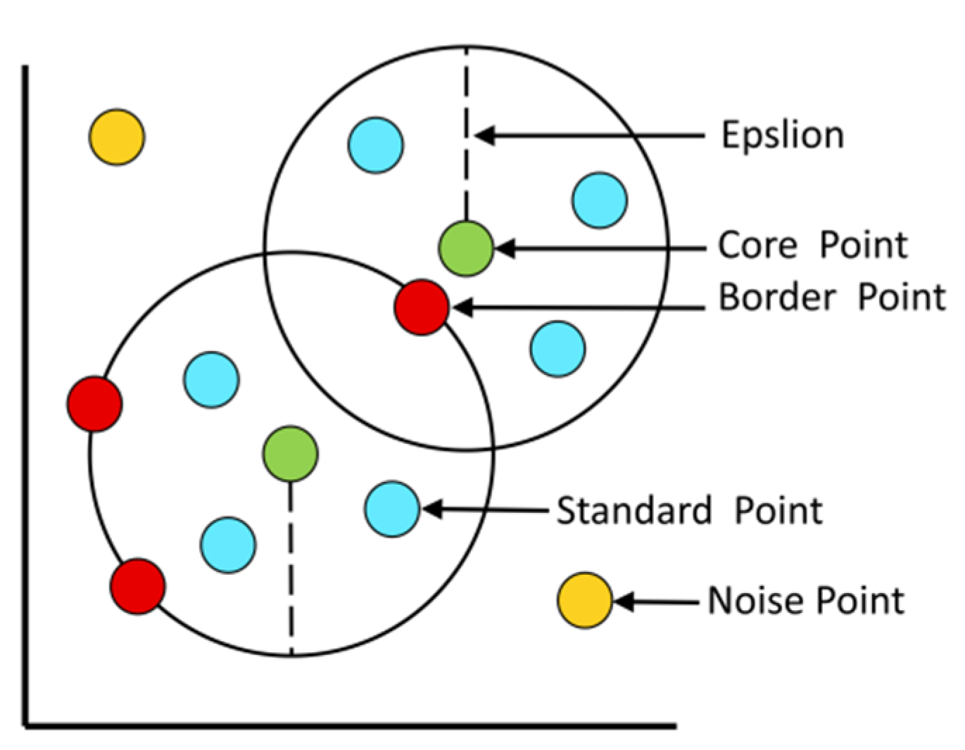
This paper introduced the DBSACAN spatial clustering algorithm for the clustering process of demand points of fresh agricultural products. On the one hand, the algorithm can accurately determine the core points, boundary points and noise points, so as to further select the standard points and improve the iterative fault tolerance and solution accuracy of the algorithm [44,45], as shown in Figure 3; on the other hand, the algorithm has no centroid, and only forms a solution set by continuously connecting high-density points in the neighborhood, which can form adaptive clustering results of different shapes and sizes.

4.1.1. Core Point Clustering

With each initial solution x as the center of a circle and Epsilon as the radius to form a neighbourhood, the solutions contained in the neighbourhood were counted. The core point xc was generated by comparison with min Pts. The equations are as follows.
N e p s i l o n ( x ) = { y X | d ( x , y ) e p s i l o n }
ρ ( x ) = | N e p s i l o n ( x ) |
x c = { x X | ρ ( x ) min P t s }
Equation (16) represents the neighbourhood of the initial solution x within the radius Epsilon and y is the reference point in the set of initial solution. d(x, y) stands for the distance from the initial solutions to the reference points in the set. Equation (17) represents the neighbourhood density of x and Equation (18) is the condition for the clustering of core point xc. All core points in set X were set Xc and the set composed of non-core points was Xnc.

4.1.2. Border, Standard and Noise Point Clustering

Based on the core points, when the number of points contained in a demand point within the neighbourhood of radius Epsilon is lower than the neighbourhood density threshold minPts, there are two cases: if the point is equal to the neighbourhood range of a certain core point xc, then the point is a boundary point xbd and the constituted set is set to Xbd, as shown in Equation (19); if the point is smaller than the neighbourhood range of a certain core point xc then the point is a standard point xst and the set formed is set to Xst, as shown in Equation (20). If a demand point does not belong to the set of core points Xc, does not belong to the set of boundary points Xbd, and also does not belong to the set of standard points Xst, then the point is a noise point xn, as shown in Equation (21).
x b d = { x X n c X c | y N e p s i l o n ( x ) d ( x , y ) = e p s i l o n ) }
x s t = { x X n c X c | y N e p s i l o n ( x ) d ( x , y ) < e p s i l o n ) }
x n = x X x X c x X b d x X s t

4.2. Improved Whale Optimization Algorithm for Iterative Solution

4.2.1. The Solution Process of the Basic Whale Optimization Algorithm

The whale optimization algorithm (WOA) is a novel heuristic algorithm of swarm intelligence proposed by Australian scholar Mirjalili in 2016 according to the behaviour of humpback whales rounding up prey [46]. The search process of the algorithm is largely divided into three stages: encircling, bubble-net attacking and spiral-shaped hunting. A solution can be represented by the position coordinates of a whale, and the process of searching for a solution can be seen as the process of several whales continuously changing their positions until the optimal solution is obtained.
(1)
Encircling
The algorithm simulates a group of humpback whales working together to locate their prey and encircle the initial solution of the target. The algorithmic model for this stage is as follows.
X k j + 1 = X k | A 1 | D k
D k = | C 1 X k X k j |
| A 1 | = 2 a r 1 a , C 1 = 2 r 2
a = 2 2 ( t / t m a x )
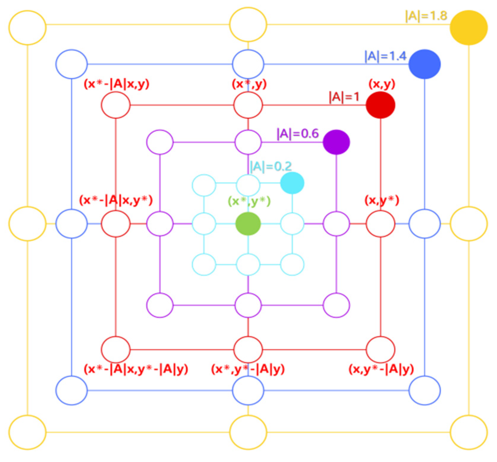
Equation (22) represents the updated position vector of other humpback whales xj after being influenced by the best humpback whale X*, and k represents the number of iterations. Equation (23) represents the distance between other whales and the best whale X* before the encirclement. Equation (24) represents that A and C are the iteration matrix coefficients. r1 and r2 are random numbers from 0 to 1. Equation (25) represents that a is an iteration parameter that decreases linearly from 2 to 0 as the number of iterations t increases. Humpback whales obtain food by controlling the |A1| vector. When |A1| ≤ 1, the whales in other positions approach the current best one.
(2)
Bubble-net attacking
As the other humpback whales move towards the best one X* to encircle the prey, they not only contract the encirclement but also follow a logarithmic spiral towards the prey. To synchronize the algorithmic operations of encircling the prey and swimming up the spiral, it was assumed that encircling is selected with 50% probability p and swimming in a spiral with 50% probability 1 − p. Equation (26) shows the mathematical model.
X k j + 1 = { X k | A 1 | D k p < 0.5 X k + D k e b l cos ( 2 π l ) p 0.5
Parameter b is a logarithmic spiral constant and l is a random number between −1 and 1. When l is close to −1, humpback whales approach the prey. Otherwise, the whales swim away.
(3)
Spiral-shaped hunting
The swimming range of a humpback whale may be |A1| > 1. At this time, other humpback whales randomly select individuals in the group to approach, which facilitates the algorithm to obtain the overall optimal solution. From this, the position iteration mechanism of the WOA algorithm under the influence of |A1| can be obtained, as shown in Figure 4.
The random individual positions of the current humpback whales were assumed as Xrand and the location of the whale to swim as Xj. The mathematical model of the behaviour of spiral-shaped hunting is shown in Equations (27) and (28).
X k j + 1 = X k r a n d | A 1 | D k
D k = | C 1 X k r a n d X k j |

4.2.2. Using Sort Matrices to Calculate the Overall Fitness of the Bi-objective Function

During the process of the location selection for cold chain distribution centers of fresh agricultural products, multiple constraints and multiple objective functions are involved, so it is difficult to measure the comparative priority of minimum total costs and minimum carbon emissions. Therefore, this paper used the comparison sort performance matrix to calculate the overall fitness of the alternative locations, in order to measure the relationship between the total costs and carbon emissions [47]. First of all, the initial value of the bi-objective function of the initial solution set Xc of the location selection for cold chain distribution centers was calculated, and the performance comparison sort of the sort matrices was carried out, which was further transformed into the overall fitness of the alternative locations. Assuming that the total costs of the location selection and the total carbon emissions during the warehousing and distribution process are Obj1 and Obj2. Their ranking numbers are OR1 and OR2 in ascending order, and the values of fitness are f1 and f2, as shown in Table 3.
The results of the performance comparison sort of the sort matrices were transformed into the individual fitness of Equations (8) and (9), in order to calculate the overall fitness of the alternative locations. The algorithm model at this stage is as follows:
f j ( i ) = { ( M O R j ( i ) ) 2 O R j ( i ) > 1 k M 2 O R j ( i ) = 1
f ( i ) = f 1 ( i ) + f 2 ( i )
Equation (29) represents the fitness value of the jth objective function. ORj(i) stands for the results of comparison sort. M is the total number of alternative locations. Equation (30) represents the overall fitness of alternative locations. K is a variable within the range of 1 to 2, which is used to increase the fitness of the optimal individual.

4.2.3. Adopting the Mutation-Induced Perturbation of the Cauchy Distribution

When the humpback whales conduct a global search in the early iterations of the algorithm, the position of the best humpback whale is needed as a guide for other whales to approach and encircle. Since the location of the best one is selected randomly by the algorithm, there is a possibility that the global optimal solution is missed. Thus, this paper adopted the mutation-induced perturbation that conforms to the Cauchy distribution [48,49,50]. Because the Cauchy distribution features wide distribution at both ends, it can make the distribution at both ends of the mutation more easily jump out of the local optimum and give full play to the effect of the mutation at both ends. In addition, during the global search by WOA, the target humpback whales are changing their coordinate positions to effectively compensate for the blindness of the mutations that conforms to the Cauchy distribution. Equation (31) shows the calculation of the Cauchy inverse cumulative distribution function.
F 1 ( p ; x 0 , γ ) = x 0 + γ tan ( π ( p 1 2 ) )
Therefore, Equation (22) can therefore be improved to Equation (32).
X k j + 1 = X m , n ( j ) + | A 1 | tan ( π ( p 1 2 ) )
In particular, F−1 represents the inverse cumulative distribution function of the Cauchy distribution. Xmn is the nth location of the mth humpback whale between the Cauchy mutation. γ = A. p is uniformly distributed within the range of 0 to 1.

4.2.4. Introducing Sine and Cosine Inertia Weights

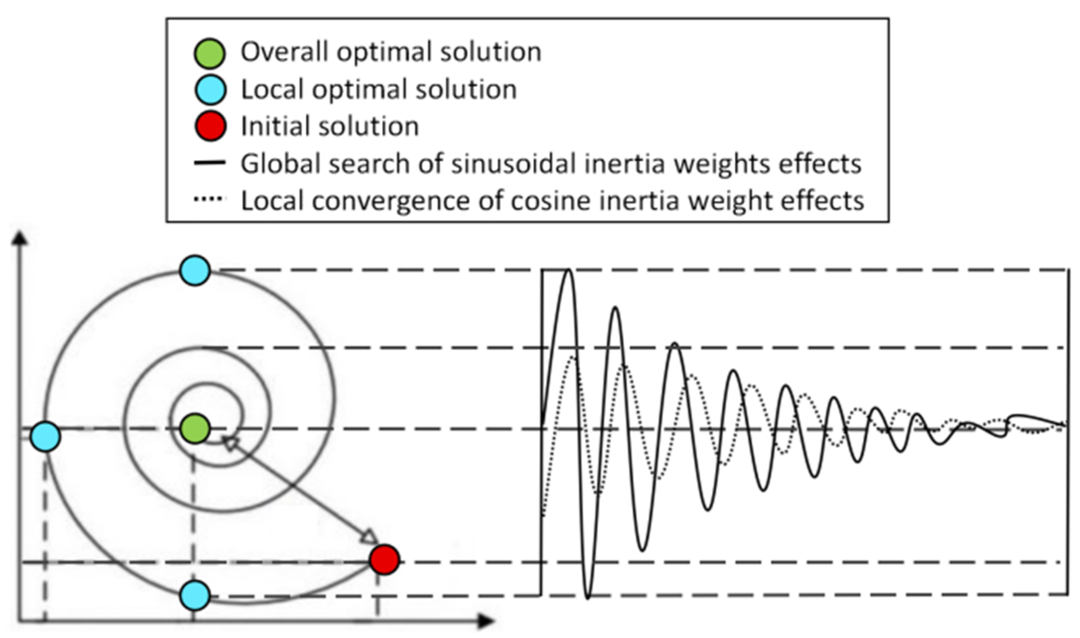
Humpback whales control the |A1| vector to move closer or farther away from the best humpback whales so as to realize the three stages of encircling, bubble-net attacking and spiral-shaped hunting. In other words, the WOA controls the search capability through the |A1| vector. The key iteration parameter a in the |A1| vector decreases linearly as the number of iterations increases. The law of the linear decreasing leads to a reduction in the convergence range in the early iterations that require a larger search range, while causing a slowdown in the rate of convergence in the later iterations that require a smaller search range, thus affecting the overall quality of convergence of the algorithm. This paper, based on the characteristics of sine and cosine curves, introduced non-linear sine and cosine inertia weights to the iteration parameter a. The search range was expanded by the sine inertia weights and the rate of convergence was enhanced by the cosine inertia weights, in order to improve the quality of convergence and population diversity of the algorithm [51,52,53]. The formulas of sine and cosine inertia weights are shown in Equations (33) and (34).
ω = ( 1 2 sin ( π t 2 T ) r 3 ) r a n d
ω = ( 1 2 cos ( π t 2 T ) r 3 ) r a n d
The control parameter r3 represents a random number in the range of 0 to 2, which is used to control the influence of the relative positions of the random humpback whales and the optimal humpback whale. The random parameter rand represents a random number in the range of 0 to 1, which is used to improve the population diversity of the algorithm. t is the current number of iterations and T is the total number of iterations, and the division of the two makes the iteration parameter a somewhat adaptive. Specifically, in the early iterations of the algorithm, the value of t/T is small and the inertia weight w is large; in the later iterations of the algorithm, t gradually converges to T, so the value of t/T is large and the inertia weight w is small. Equation (32) can be therefore improved to Equation (35).
X k j + 1 = X m , n ( j ) + ω | A 1 | tan ( π ( p 1 2 ) )
Figure 5 shows the influence of the |A1| vector under sine and cosine inertia weights on the global search and local convergence of the hunting of the humpback whales in different iteration cycles of the one-dimensional hunting space.
The solid line represents the situation of shunting under the influence of sine inertia weights. The target humpback whale moves in a sinusoidal logarithmic spiral trajectory guided by the random individual Xrand of the population. A global search is carried out before the stage of spiral-shaped hunting, reducing the blind spot of the small local convergence range of the cosine inertia weights and avoiding the situation where the potential optimal solution is missed. The dotted line represents the situation of shunting under the influence of cosine inertia weights. The target humpback whale moves in a cosine logarithmic spiral trajectory guided by the best humpback whale X*. A local convergence takes place at the late stage of spiral-shaped hunting, which compensates for the slow convergence of the global search of sine inertia weights and improves the operation efficiency of the algorithm.

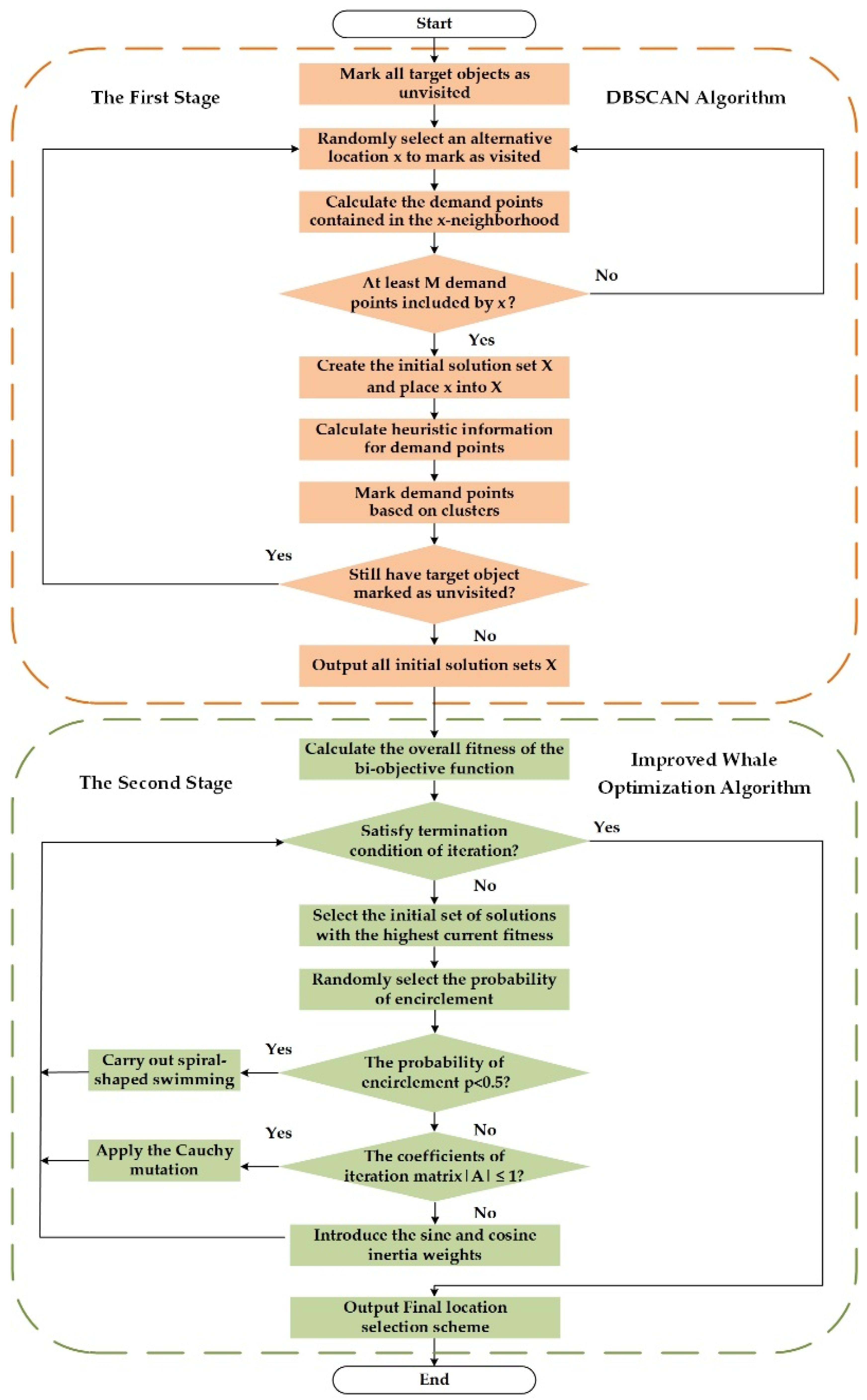
4.3. Solving Steps of Two-Stage Heuristic Algorithm

The specific algorithm flow is shown in Figure 6.
The first stage heuristic Algorithm 1 steps are as follows:
Algorithm 1 First stage
  Import the necessary class library files
  Define key variables and parameters
  BEGIN
    Click the Start button
    Sign () function marks all objects as unvisited
    The random function Random () determines an alternative point as x
    Assign the x attribute to visited X = visited
    Calculate N demand points in x field
    If (N>=M)
    {
     Create solution set X
     X. add (x)
     Computational heuristic information
     Cluster() clustering algorithm marks demand points
     If (still target object unvisited)
     {
      Execute random function Random() module
     }else
     {
      Output all initial solution sets X
     }
    }else
    {
      Re-execute the random function Random() module
    }
  END
The second stage heuristic Algorithm 2 steps are as follows:
Algorithm 2 Second stage
  Import the necessary class library files
  Define key variables and parameters
  BEGIN
    According to the solution set X of the previous algorithm
    Calculate() calculate the overall fitness of the bi-objective function
    If (iteration termination condition satisfied)
    {
     Output program results
    }
    Else
    {
     The MAX() function selects the initial solution set with the highest fitness
     The Random() function randomly selects the corresponding probability P
     If (probability P<0.5)
     {
      Carry out spiral-shaped swimming
      Determine whether the iteration termination condition is satisfied
      Perform corresponding operations
     }
     Else
     {
      If (|A|<=1)
      {
       Apply the Cauchy mutation
       Determine whether the iteration termination condition is satisfied
       Perform corresponding operations
      }
      Else
      {
       Introduce the sine and cosine inertia weights
       Determine whether the iteration termination condition is satisfied
       Perform corresponding operations
      }
     }
    }
  END

5. Case Description and Data Acquisition

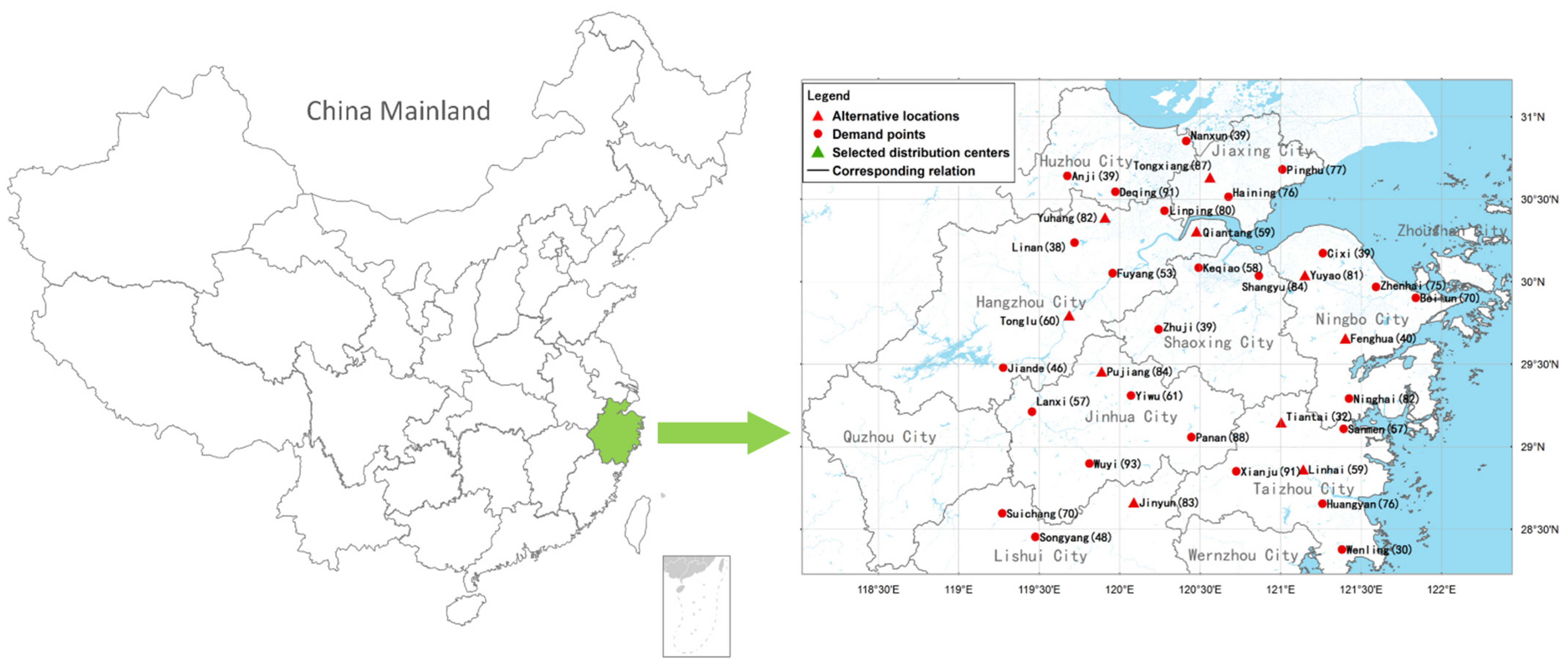
To test the effectiveness and feasibility of the two-phase heuristic algorithm in the actual location selection process, a case study was selected as follows. Y enterprise in Zhejiang Province, in order to meet the daily demands of fresh agricultural products of 36 regional demand points [54,55], decided to establish a number of cold chain distribution centers in order to provide integrated services, taking carbon emission and sustainable development into account. Among the 36 demand points, 10 were selected as alternative locations, including 1 Yuhang District, 5 Qiantang District, 7 Tonglu County, 10 Fenghua District, 11 Yuyao City, 22 Tongxiang City, 26 Pujiang County, 29 Linhai City, 32 Tiantai County and 34 Jinyun County, among which six locations had to be selected to build a cold chain distribution center and optimize the address. Table 4 shows the Zhejiang Y enterprise’s demand points for fresh agricultural products and the corresponding demands.
The demand points of the Zhejiang Y enterprise distributed in 36 regions were divided, and the demands in each region were summed up as the transportation volume of the demand point. To facilitate the solution of the straight-line distance dij from the alternative location i of a cold chain distribution center to the target demand point j, this paper used the ArcGIS software to convert the latitude and longitude coordinate data into plane coordinate data, as shown in Figure 7.
In the actual location selection, high storage cost per unit of goods and the fixed reconstruction costs of the alternative locations are important factors affecting the total costs. The data related to the alternative locations for cold chain distribution centers of fresh agricultural products of the Zhejiang Y enterprise are shown in Table 5.
According to the relevant data, the relevant parameters assumed of refrigerated vehicles in the process of cold chain warehousing and distribution of fresh agricultural products are shown in Table 6.
According to IPCC’s proposal, the carbon price was USD 30 per ton in 2020 [56] (USD 0.03/kg·CO2). Therefore, this paper assumes that the current cost per unit of carbon emissions in Zhejiang Province is 0.03 dollar/kg·CO2. Based on relevant data, the values of other constants are assumed as shown in Table 7.

6. Results and Discussion

6.1. Contrastive Analysis of the Case Study

In order to verify the efficiency of the two-phase heuristic algorithm (THA) proposed in this paper for solving the location selection for cold chain distribution centers of fresh agricultural products, a simulation comparison was conducted on THA, the basic whale optimization algorithm [57,58] (WOA) and the basic particle swarm optimization algorithm [59,60] (PSO) through the case of Y enterprise in Zhejiang Province. The experimental platform for the simulation was Win11, and MATLAB R2021b software was used for the operation.
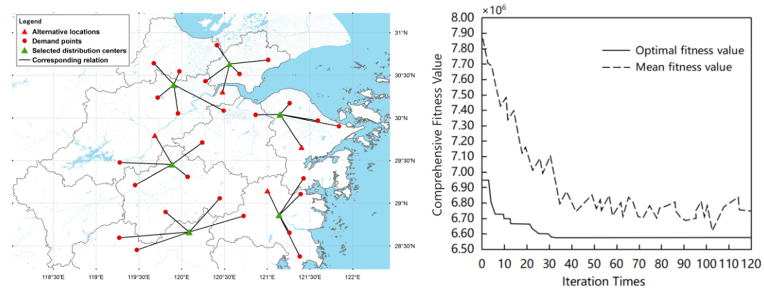
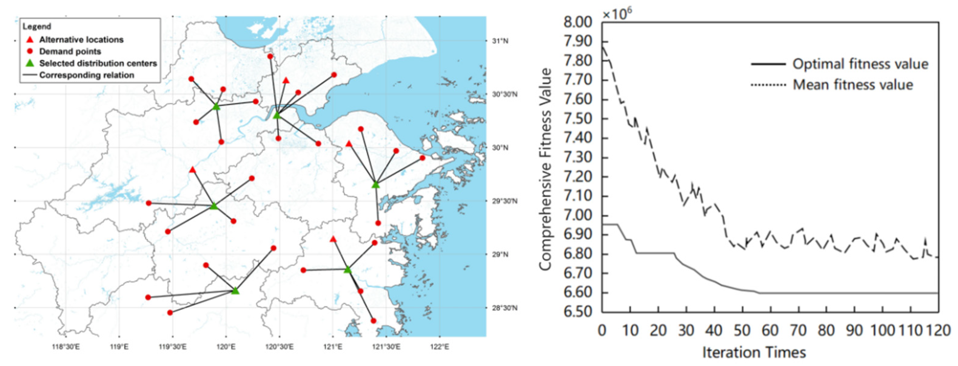
The number of population N was 36, and the maximum number of iterations T was 200. The neighbourhood density radius Epsilon was 100 km, and the neighbourhood density threshold minPts was a natural number 6 in the DBSCAN algorithm. The probability of encirclement p was 0.5 and the probability of mutation-induced perturbation of the Cauchy Distribution pγ was 0.3 in the IWOA algorithm. The locations of cold chain distribution centers obtained by the three algorithms and the final optimization results of the experiment are shown in Table 8. The effect pictures of the location selection and the iterative convergence curves of the three algorithms are shown in Figure 8, Figure 9 and Figure 10. Figure 11 presents the iterative convergence contrast curves of the three algorithms, and Figure 12 shows the changing curves of the overall carbon emissions during the location selection process of the three algorithms.
According to the comparison of the performance of the three algorithms in the location selection shown in Table 8, in terms of the total costs of the location selection, the THA algorithm’s average optimization is 7.70% compared with the WOA algorithm and 12.77% compared with the PSO algorithm. In terms of the overall carbon emissions, the THA algorithm’s average optimization rate is 10.23% compared with the WOA algorithm and 14.12% compared with the PSO algorithm. It is suggested that the THA algorithm matches a better location selection scheme with fewer iterations under the constraint of the same cost per unit of carbon emissions.
According to the location selection scheme and the comparison of iterative convergence shown in Figure 8, Figure 9, Figure 10, Figure 11 and Figure 12, the search process of the WOA and PSO algorithms is significantly broken and stagnant in the early iterations, indicating that the local optimum has occurred, while the iterative performance of the THA algorithm is more continuous and smooth, and the fitness decreases more quickly, which means it has a more efficient iteration capability. At the late stage of algorithm iteration, both the WOA and PSO algorithms enter a bottleneck to some extent and differ significantly from the THA algorithm in terms of effectiveness and continuity of iteration.

6.2. Sensitivity Analysis Based on the Cost per Unit of Carbon Emissions

In order to verify the impact of the cost per unit of carbon emissions on the total costs of location selection during the process of warehousing and distribution, this paper used an analysis method with control variables and a two-phase heuristic algorithm to change the cost per unit of carbon emissions to carry out a multi-group controlled experiment while other constant parameters remained unchanged. Assuming a cost per unit of carbon emissions of 0.02 dollar/kg as the starting point and an incremental rule of 0.01 dollar/kg, a sensitivity analysis based on carbon emissions was conducted and the changes in the overall carbon emission costs and the total costs of location selection are shown in Table 9.
According to Table 9, as the cost per unit of carbon emissions increases, both the overall carbon emission costs and the total costs of location selection show an upward trend, with the former accounting for a bigger proportion of the total costs. It is further verified that the cost per unit of carbon emissions and the total costs are significantly positively correlated, and the two-phase heuristic algorithm can effectively obtain locations for cold chain distribution centers of fresh agricultural products under carbon emission constraints. As people pay much attention to environmental protection, the cost per unit of carbon emissions will continue to rise [61]. It will be an inevitable choice for enterprises to take efficient energy-saving and emission-reduction measures in order to reduce costs and increase efficiency in the future.

7. Conclusions

Based on the traditional location for distribution centers, this paper optimized for both freshness and carbon emissions. A bi-objective function model was constructed to minimize the total cost and the carbon emission. The total cost consists of four com-ponents: the cost of storage, the cost of transportation, the cost of freshness penalty and the comprehensive carbon emission cost. The carbon emission consists of two compo-nents: the static carbon emission of the cold chain distribution centers and the dynamic carbon emission of the refrigerated vehicles transportation. A two-stage heuristic algo-rithm was designed to solve the model: the first stage used the DBSCAN algorithm to divide the initial solution set and the second stage used the IWOA to obtain the overall optimal solution.
The results of the case of enterprise Y in Zhejiang Province verified the feasibility of the model and the main conclusions obtained include: first, the THA had an average total cost optimization rate of 7.70% and an average carbon emission optimization rate of 10.23% compared to the WOA, while it had rates of 12.77% and 14.12%, respectively, compared to the PSO. This shows that the THA can significantly optimize the solution results. Second, the unit carbon emission cost affected the location for cold chain distribution centers. When the unit carbon emission cost increased from 0.02 dollar/kg to 0.06 dollar/kg, the overall carbon emission cost increased by 42.07%, the total cost increased by 3.05% and the proportion of overall carbon emission cost in the total cost increased from 2.21% to 3.05%. Therefore, logistics enterprises can reduce the total cost through reasonable location for fresh agricultural products cold chain distribution centers [45,46].
Further research can apply the two-stage heuristic algorithm to the two-level planning for location of fresh agricultural products cold chain distribution centers and the route optimization of refrigerated vehicles [62,63,64,65]. The impact of time window constraints at demand points [66] and traffic condition constraints [67] on the planning of cold chain logistics systems can also be considered. In addition, the author will focus on this type of problem in the future.

Author Contributions

All of the authors contributed to the work in the paper. Specifically: Conceptualization, H.W. and H.R.; methodology, H.W. and H.R.; software, H.W., H.R. and X.D.; validation, H.W., H.R. and X.D.; data curation, H.W. and X.D.; writing—original draft preparation, H.W. and H.R.; writing—review and editing, H.W. and H.R.; funding acquisition, H.W. and X.D. All authors have read and agreed to the published version of the manuscript.

Funding

The research was supported by Shandong Province Social Science Project (No. 18CGLJ35), 2019 Shandong Humanities and Social Sciences Project (No. 19-ZZ-GL-09), 2019 Qingdao Social Science Planning Research Project (QDSKL1901168).

Data Availability Statement

The relevant data of this research work can be obtained by contacting the author.

Conflicts of Interest

The authors declare no conflict of interest.

References

  1. Wang, H.J.; Chen, P.Y. A review of research on cold chain logistics and distribution of fresh agricultural products. Coop. Econ. Technol. 2022, 4, 93–95. [Google Scholar] [CrossRef]
  2. Luo, Y.; Peng, Y. Analysis on the development strategy of cold chain logistics of fresh agricultural products. Mod. Agric. Technol. 2022, 5, 203–204, 207. [Google Scholar]
  3. Mao, X.Y. Research on the development problems and solutions of fresh cold chain logistics in the post-epidemic era. China Storage Transp. 2022, 2, 185–187. [Google Scholar] [CrossRef]
  4. Yu, S.Z. Risk Assessment of Fresh Food E-Commerce Cold Chain Logistics. Master’s Thesis, Shijiazhuang Railway University, Shijiazhuang, China, 2021. [Google Scholar]
  5. Zhang, S. Research on Risk Identification, Evaluation and Countermeasures of Cold Chain Logistics of Fresh Agricultural Products. Master’s Thesis, Anhui University of Science and Technology, Hefei, China, 2020. [Google Scholar]
  6. Lord, H.E.; Taylor, J.D.; Finn, J.C.; Tsokos, N.; Jeffery, J.T.; Atherton, M.J.; Evans, S.F.; Bremner, A.P.; Elder, G.O.; Holman, C.D.A.J. A randomized controlled equivalence trial of short-term complications and efficacy of tension-free vaginal tape and suprapubic urethral support sling for treating stress incontinence. BJU Int. 2006, 98, 367–376. [Google Scholar] [CrossRef] [PubMed]
  7. Zhang, S.Y.; Chen, N.; Li, Y.H.; Yang, J. Research on optimization decision-making of urban cold chain logistics distribution system from the perspective of low carbon. Ind. Eng. Manag. 2022, 27, 56–64. [Google Scholar] [CrossRef]
  8. Duan, S.Y. Location-Path Research on Cold Chain Distribution of Fresh Agricultural Products Considering Carbon Trading. Master’s Thesis, Beijing Jiaotong University, Beijing, China, 2019. [Google Scholar]
  9. Pei, Y.H. Research on Location Selection of Cold Chain Distribution Center for Fresh Agricultural Products Based on Demand Forecast. Master’s Thesis, Chongqing Technology and Business University, Chongqing, China, 2016. [Google Scholar]
  10. Li, X.; Zhou, K. Multi-objective cold chain logistic distribution center location based on carbon emission. Environ. Sci. Pollut. Res. 2021, 28, 32396–32404. [Google Scholar] [CrossRef]
  11. Jiang, Y.M.; Wang, S.Y.; Ma, X.L. Research on the cold chain logistics system of agricultural products based on carbon optimization. Technol. Manag. Res. 2017, 37, 221–227. [Google Scholar]
  12. Tian, L.N. Optimization Analysis of Fruit Single-Stage Cold Chain Benefit Considering Carbon Emissions. Master’s Thesis, Southwest Jiaotong University, Chongqing, China, 2012. [Google Scholar]
  13. Benjaafar, S.; Li, Y.; Daskin, M. Carbon footprint and the management of supply chains: Insights from simple models. IEEE Trans. Autom. Sci. Eng. 2013, 10, 99–116. [Google Scholar] [CrossRef]
  14. Pan, Q.Q.; Gan, H.C. Research on optimization of cold chain logistics distribution path considering carbon emissions. Pract. Underst. Maths 2016, 46, 62–68. [Google Scholar]
  15. Li, H.D. Research on Inventory-Distribution Strategy of Fresh Food Supply Chain under Different Decision-Making Modes. Master’s Thesis, Beijing Jiaotong University, Beijing, China, 2020. [Google Scholar]
  16. Weber, A. Ueber Den Standort Der Industrien; Wentworth Press: London, UK, 1922. [Google Scholar]
  17. Hakimi, S.L. Optimum Locations of Switching Centers and the Absolute Centers and Medians of a Graph. Oper. Res. 1964, 12, 450–459. [Google Scholar] [CrossRef]
  18. Kayikci, Y. A conceptual model for intermodal freight logistics center location decisions. Procedia-Soc. Behav. Sci. 2010, 2, 6297–6311. [Google Scholar] [CrossRef] [Green Version]
  19. Fu, X.P.; Zou, J. Application of analytic hierarchy process in location selection of logistics center. World Shipp. 2002, 4, 23–24, 28. [Google Scholar]
  20. He, F.Z. Research and Application of Logistics Park Location Decision-Making. Master’s Thesis, Chongqing University, Chongqing, China, 2006. [Google Scholar]
  21. Zheng, Z.C.; Liu, X. The application of grey correlation degree and AHP in cold chain logistics distribution center location problem. Sci. Technol. Eng. 2009, 9, 1366–1369, 1374. [Google Scholar]
  22. Lu, X.C.; Zhan, H.S. Research on location selection of distribution center by gravity center method. J. North. Jiaotong Univ. 2000, 6, 108–110. [Google Scholar]
  23. Hua, G.W.; Yang, F.M.; Li, J.Q. Two two-objective competitive location problem models. Syst. Eng. Theory Pract. 2007, 1, 99–106. [Google Scholar]
  24. Li, Z.Y.; Lin, H.; Li, W. Layout of distribution center of fresh supermarket chain based on Baumol-Wolfe method. Logist. Technol. 2005, 7, 19–23. [Google Scholar]
  25. Erlebacher, S.J.; Meller, R.D. The interaction of location and inventory in designing distribution systems. IIE Trans. Inst. Ind. Eng. 2000, 32, 155–166. [Google Scholar] [CrossRef]
  26. Jiang, D.L.; Du, W. Location model of logistics distribution center based on genetic algorithm. Logist. Technol. 1997, 5, 3–6. [Google Scholar]
  27. Shen, B. Application of Improved Ant Colony Algorithm in Logistics Distribution. Master’s Thesis, Zhejiang University, Hangzhou, China, 2004. [Google Scholar]
  28. Yang, B. Research on Application of Tabu Search Algorithm in Refrigerated Supply Chain Distribution Network. Master’s Thesis, Shanghai Maritime University, Shanghai, China, 2005. [Google Scholar]
  29. Bai, S.; Liu, X. Research on Location of Cold Logistic Chains Distribution Centers Based on Grey Correlation Degree and AHP Method. In Proceedings of the 2008 IEEE International Conference on Service Operations and Logistics, and Informatics, Beijing, China, 12–15 October 2008; Volume 2, pp. 3027–3030. [Google Scholar]
  30. Pan, Q. Research on Location Selection of Cold Chain Distribution Center Based on Two-Level Planning Model. Master’s Thesis, Wuhan University of Technology, Wuhan, China, 2013. [Google Scholar]
  31. Montanari, R. Cold chain tracking: A managerial perspective. Trends Food Sci. Technol. 2008, 19, 425–431. [Google Scholar] [CrossRef]
  32. Demirtaş, N.; Tuzkaya, U.R. Strategic planning of layout of the distribution center: An approach for fruits and vegetables hall. Procedia-Soc. Behav. Sci. 2012, 58, 159–168. [Google Scholar] [CrossRef] [Green Version]
  33. Li, X.; Wu, X.B.; Liu, Q. Location model of logistics distribution center based on variation and dynamic adaptive PSO. J. Dali Univ. 2021, 6, 12–16. [Google Scholar]
  34. Tang, X.F.; He, J.; Zhang, H. A two-stage site-routing problem considering carbon emissions and its algorithm. J. Southwest Jiaotong Univ. 2022, 4, 1–7. [Google Scholar]
  35. Li, J.J. Research on Location Selection of Cold Chain Logistics Distribution Center for Fresh Agricultural Products. Master’s Thesis, North Central University, Taiyuan, China, 2021. [Google Scholar]
  36. Yin, W.W. A case study on location selection of logistics distribution center. Logist. Eng. Manag. 2020, 42, 23, 68–71. [Google Scholar]
  37. Li, G.Q. Site Selection-Inventory-Path Integration Optimization and Research of Logistics System in Stochastic Environment. Master’s Thesis, Lanzhou Jiaotong University, Lanzhou, China, 2019. [Google Scholar]
  38. Wang, Y.Q.; Zhou, Y.; Zhang, R. Research on the equilibrium model of multi-level cold chain logistics network for agricultural products considering carbon emissions. J. Beijing Jiaotong Univ. 2017, 16, 99–107. [Google Scholar] [CrossRef]
  39. Wang, M. Research on Optimization Model and Algorithm of Fresh Product Logistics Distribution Considering Freshness. Master’s Thesis, Dalian University of Technology, Dalian, China, 2018. [Google Scholar]
  40. Ma, R.F. Research on the Equilibrium of Logistics Service Supply Chain Network Considering Carbon Emission and Carbon Emission Reduction Cost Allocation. Master’s Thesis, Qingdao University, Qingdao, China, 2021. [Google Scholar]
  41. Fei, X.D. Research on Vehicle Routing Problem in Cold Chain Logistics Distribution of Fresh Agricultural Products. Master’s Thesis, Beijing University of Posts and Telecommunications, Beijing, China, 2021. [Google Scholar]
  42. Hu, Y.L.; Zhu, Q.Y. Analysis on the revision of the waste volume of “IPCC 2006 Guidelines for National Greenhouse Gas Inventories” (2019 Revised Edition). Low Carbon World 2021, 11, 49–50. [Google Scholar] [CrossRef]
  43. Bowyer, D.P.; Akçelik, R.; Biggs, D.C. Guide to Fuel Consumption Analyses for Urban Traffic Management; Australian Road Research Board: Sydney, Australia, 1984. [Google Scholar]
  44. Zhao, Z.Q.; Zhang, L.T.; Wang, W.Z.; Hu, Z.B. Research on location selection of fresh agricultural products front warehouse based on customer demand distribution. Comput. Appl. Softw. 2021, 38, 107–113, 124. [Google Scholar]
  45. Sun, L.; Liang, Y.Q. An improved clustering algorithm integrating meshing and DBSCAN. Comput. Eng. Appl. 2022, 4, 1–9. [Google Scholar]
  46. Mirjalili, S.; Lewis, A. The whale optimization algorithm. Adv. Eng. Softw. 2016, 95, 51–67. [Google Scholar] [CrossRef]
  47. Dong, X.H. Research on Low-Carbon Distribution Path Selection of Fresh Agricultural Products Cold Chain Under Time-Varying Road Network. Master’s Thesis, Tianjin University of Technology, Tianjin, China, 2021. [Google Scholar]
  48. Shang, M.; Kang, J.Y.; Cao, J.W.; Wang, Z.P. Location strategy of logistics distribution center based on improved whale optimization algorithm. Comput. Appl. Softw. 2019, 36, 254–259. [Google Scholar]
  49. Qiu, X.G.; Wang, R.Z.; Zhang, W.G.; Zhang, Z.Z.; Zhang, Q. Improved whale optimization algorithm based on mixed strategy. Comput. Eng. Appl. 2022, 58, 70–78. [Google Scholar]
  50. Guo, Z.Z.; Wang, P.; Ma, Y.F.; Wang, Q.; Gong, C.Q. Whale optimization algorithm based on adaptive weights and cauchy variation. Microelectron. Comput. 2017, 34, 20–25. [Google Scholar] [CrossRef]
  51. Liu, Z.S.; Li, S. Positive co-chaos double string whale optimization algorithm. Comput. Eng. Appl. 2018, 54, 159–163, 212. [Google Scholar]
  52. Wang, Y.B. E-commerce logistics distribution path planning based on improved sine and cosine algorithm. J. Taiyuan Univ. 2021, 39, 68–74. [Google Scholar] [CrossRef]
  53. Shi, C.H.; Liu, H. Pharmaceutical logistics distribution path planning based on sine and cosine adaptive gray wolf optimization algorithm. Pract. Underst. Math. 2020, 50, 114–127. [Google Scholar]
  54. Ren, J. A review of research on cold chain logistics and distribution of fresh agricultural products in my country. Logist. Technol. 2022, 45, 150–152. [Google Scholar] [CrossRef]
  55. Zhang, D.Y. Research on the Supply Chain Model of Fresh Agricultural Products in enterprise Province. Master’s Thesis, Shanghai Academy of Social Sciences, Shanghai, China, 2018. [Google Scholar]
  56. Zhou, T.J.; Chen, X.L. Analysis on the accurate estimation of future carbon emission space under the temperature control target of the “Paris Agreement”. Proc. Chin. Acad. Sci. 2022, 37, 216–229. [Google Scholar] [CrossRef]
  57. Wu, H.J. Distribution route planning of agricultural product logistics enterprises based on greedy whale optimization algorithm. J. Lanzhou Inst. Technol. 2022, 29, 83–87. [Google Scholar]
  58. Tang, L.Q.; Ying, Z.Y.; Luo, Y. Base station location selection based on whale optimization and improved algorithm. Comput. Mod. 2020, 9, 100–105. [Google Scholar]
  59. Li, X.; Wu, X.B.; Tong, B.L. Particle swarm optimization algorithm based on dynamic adaptive variable parameters. J. Sichuan Univ. Light Chem. Ind. 2021, 34, 41–47. [Google Scholar]
  60. Gao, X.X. Several Particle Swarm Optimization Algorithms and Their Applications. Master’s Thesis, Northern University for Nationalities, Yinchuan, China, 2020. [Google Scholar]
  61. Hao, Y.T. Research on Cold Chain Coordination under Carbon Allowance Trading Mechanism. Master’s Thesis, North China Electric Power University, Beijing, China, 2021. [Google Scholar]
  62. Zheng, J.Z.; Hong, Y.W.; Xu, W.C.; Li, W.T.; Chen, Y.F. An effective iterated two-stage heuristic algorithm for the multiple Traveling Salesmen Problem. Comput. Oper. Res. 2022, 143, 105772. [Google Scholar] [CrossRef]
  63. He, L. Research on Dynamic Vehicle Routing Optimization Based on Two-Stage Heuristic Algorithm. Master’s Thesis, Chongqing University of Posts and Telecommunications, Chongqing, China, 2021. [Google Scholar]
  64. Luan, L. Research on Location Selection and Path Optimization of Cold Chain Distribution Center for Fresh Agricultural Products Based on Double-Layer Planning. Master’s Thesis, Beijing Jiaotong University, Beijing, China, 2019. [Google Scholar]
  65. Linfati, R.; Escobar, J.W.; Escalona, J. A two-phase heuristic algorithm for the problem of scheduling and vehicle routing for delivery of medication to patients. Math. Probl. Eng. 2018, 2018, 8901873. [Google Scholar] [CrossRef]
  66. Pan, L.G. Model Research on Low-Carbon Multimodal Transport Routing Problem Considering Time Window. Master’s Thesis, Nanjing University, Nanjing, China, 2020. [Google Scholar]
  67. Sun, J.P. Research on Route Optimization of Cold Chain Logistics Considering Traffic Congestion and Time Window Constraints. Master’s Thesis, North China Electric Power University, Beijing, China, 2021. [Google Scholar]
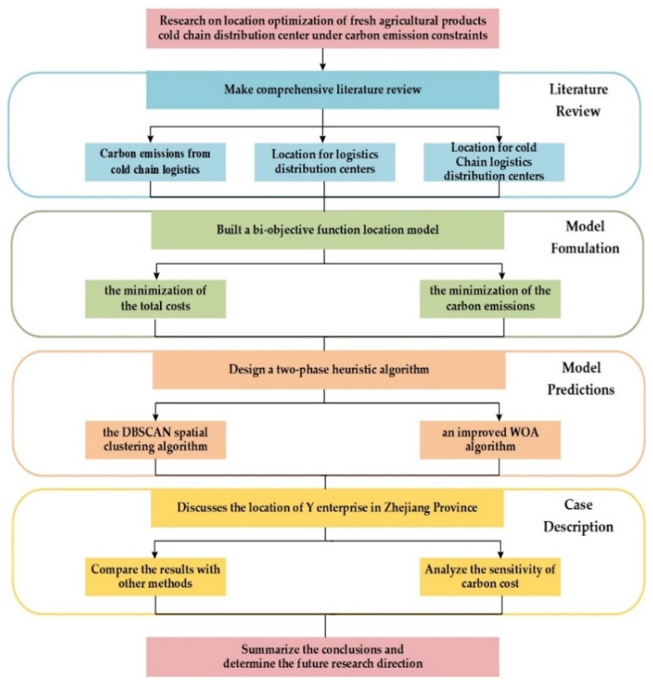
Figure 1. The overall research framework diagram.
Sustainability 14 06726 g001
Figure 2. The functional relationship between freshness of fresh agricultural products and time.
Sustainability 14 06726 g002
Figure 3. The relative distribution position of the core parameters of the DBSCAN algorithm.
Sustainability 14 06726 g003
Figure 4. The position iteration mechanism controlled by |A1| in WOA algorithm.
Sustainability 14 06726 g004
Figure 5. The solution mechanism of WOA algorithm under sin-cos inertial weight in one-dimensional space.
Sustainability 14 06726 g005
Figure 6. The two-stage heuristic algorithm flow.
Sustainability 14 06726 g006
Figure 7. The Plane cartesian coordinate system based on latitude and longitude of Y enterprise’s demand points.
Sustainability 14 06726 g007
Figure 8. The effect pictures of location selection and iterative convergence curves of the THA algorithm.
Sustainability 14 06726 g008
Figure 9. The effect pictures of location selection and iterative convergence curves of the WOA algorithm.
Sustainability 14 06726 g009
Figure 10. The effect pictures of location selection and iterative convergence curves of the PSO algorithm.
Sustainability 14 06726 g010
Figure 11. The iterative convergence contrast curves of the three algorithms.
Sustainability 14 06726 g011
Figure 12. The overall carbon emissions contrast curves of the three algorithms.
Sustainability 14 06726 g012
Table 1. Hypothetical premise in the model.
Hypothetical SituationsContent
Supply and Demand(1) the inventory of a single distribution center can satisfy the demand of covering demand points, and the inventory is equal to the sum of the demand of all demand points
(2) the demand for fresh agricultural products at each demand point is fixed and will not fluctuate greatly in the short term
Transportation(1) alternative locations are equipped with sufficient refrigerated vehicles for transport, regardless of shipping batches and fixed costs of vehicles
(2) refrigerated vehicles travel at a constant speed, regardless of service time window constraints and vehicles routing
Carbon Emissions(1) the site selection process involves static carbon emissions from distribution centers and dynamic carbon emissions from refrigerated vehicle transportation
(2) carbon emissions from product decay are not considered
Freshness(1) the freshness of fresh agricultural products is only related to the transportation time
(2) the effect of temperature change on freshness is not considered
Table 2. Symbols and variables in the model.
Parameters and SymbolsMeaning
nthe number of demand points of fresh agricultural products
mthe number of alternative locations for distribution centers
hthe number of distribution centers to be established
fithe fixed reconstruction costs of the alternative location i for distribution centers
qijthe quantity of products provided by i to the demand point j
Djthe quantity of products that j needs to provide
cithe storage cost per unit of goods stored in i
dijthe straight-line distance between i and j
cothe fuel cost per unit distance during transportation
λthe cost per unit of carbon emissions
ECithe electric energy consumed by i
e1carbon emission factor per unit of electricity consumed
e2carbon emission factor per unit of diesel consumed
OPithe amount of diesel consumed in daily storage operations in i
δ1the low calorific value of diesel
δ2carbon content per unit calorific value of diesel
δ3the carbon oxidation factor of diesel
VPthe diesel consumption per unit distance travelled by a refrigerated vehicle
Q0the weight of a refrigerated vehicle
Qmaxthe maximum load of a refrigerated vehicle
β1the penalty cost for fresh agricultural products
that do not meet the freshness requirements of the demand points
β2the negative penalty cost for fresh agricultural products
that meet the freshness requirements of the demand points
Rthe freshness of fresh agricultural products when delivered to the demand points
Φthe sensitivity coefficient of freshness to time
Δtthe time needed for the transportation of fresh agricultural products
to the point of demand
yia 0/1 variable. If a cold chain distribution center is established on i,
yi is 1, otherwise, it is 0
xija 0/1 variable. If i serves j, xij is 1, otherwise, it is 0
a&bthe linear parameters
Table 3. Performance comparison ranking of ranking matrices for bi-objective function.
ObjectAlternative
Al(1)Al(2)Al(3)Al(M)
Obj1OR1(1)OR1(2)OR1(3)OR1(M)
Obj2OR2(1)OR2(2)OR2(3)OR2(M)
Table 4. Y enterprise’s demand points for fresh agricultural products and the corresponding demands.
Demand PointsLongitude and Latitude CoordinatesDemanded Quantity/tDemand PointsLongitude and Latitude CoordinatesDemanded Quantity/t
1 Yuhang District(120.30, 30.42)8219 Anji County(119.68, 30.63)39
2 Fuyang District(119.95, 30.05)5320 Pinghu City(121.02, 30.70)77
3 Linan District(119.72, 30.23)3821 Haining City(120.68, 30.53)36
4 Linping District(120.30, 30.43)8022 Tongxiang City(120.57, 30.63)87
5 Qiantang District(120.22, 30.26)5923 Lanxi City(119.45, 29.22)57
6 Jiande City(119.28, 29.48)4624 YiwuCity(120.07, 29.30)61
7 Tonglu County(119.67, 29.80)6025 Wuyi County(119.82, 28.90)93
8 Beilun District(121.85, 29.93)7026 Pujiang County(119.88, 29.45)84
9 Zhenhai District(121.72, 29.95)7527 Pan’an County(120.43, 29.05)88
10 Fenghua District(121.40, 29.65)4028 Huangyan District(121.27, 28.65)76
11 Yuyao City(121.15, 30.03)8129 LInhai City(121.12, 28.85)59
12 Cixi City(121.23, 30.17)3930 WenLingCity(121.37, 28.37)30
13 Ninghai County(121.43, 29.28)8231 Sanmen County(121.38, 29.12)57
14 Keqiao District(120.50, 30.08)5832 Tiantai County(121.03, 29.13)32
15 Shangyu District(120.87, 30.03)8433 Xianju County(120.73, 28.87)91
16 Zhuji City(120.23, 29.72)3934 Jinyun County(120.07, 28.65)83
17 Nanxun City(120.43, 30.88)3935 Suichang County(119.27, 28.60)70
18 Deqing County(119.97, 30.53)9136 Songyang County(119.48, 28.45)48
Table 5. Data related to Y enterprise’s alternative locations for cold chain distribution centers.
Alternative LocationStorage Cost per Unit of Goods ci/DollarFixed Reconstruction Costs fi/10,000 DollarElectric Energy Consumption ECi/kw×hDiesel Consumption OPi/kg
1 Yuhang District137.225.40232428
5 Qiantang District145.465.70203336
7 Tonglu County110.977.50220432
10 Fenghua District134.224.05234134
11 Yuyao City130.473.15206334
22 Tongxiang City138.726.15219121
26 Pujiang County122.976.90230435
29 LInhai City117.725.25210021
32 Tiantai County127.474.65207530
34 Jinyun County119.226.15239439
Table 6. Relevant parameters of Y enterprise’s refrigerated vehicles.
VariableValueUnit
the fuel cost per unit distance during transportation co0.27dollar/km
the speed of the vehicle v40km·h−1
the diesel consumption of empty vehicles VP00.14kg·km−1
the diesel consumption of fully-loaded vehicles VPmax0.16kg·km−1
the weight of a refrigerated vehicle Q032,000kg
the maximum load of a refrigerated vehicle Qmax50,000kg
Table 7. Other constant values related to the model.
ConstantValueUnit
carbon emission factor per unit of electricity consumed e10.5810tCO2·MW·h−1
carbon emission factor per unit of diesel consumed e23.0959kg-CO2·kg−1
the low calorific value of diesel δ142652kJ·kg−1
carbon content per unit calorific value of diesel δ220.20t-C·TJ−1
the carbon oxidation factor of diesel δ30.98unitless
the cost per unit of carbon emissions λ0.03dollar/kg·CO2
the penalty cost when the freshness requirements are not met β1119.97dollar
the negative penalty cost when the freshness requirements are met β2119.97dollar
the sensitivity coefficient of freshness to time φ1.60unitless
Table 8. Comparison of the performance of the three algorithms in the location selection.
AlgorithmTHAWOAPSO
the location of the cold chain distribution center(1, 11, 22, 26, 29, 34)(1, 5, 10, 26, 29, 34)(5, 7, 11, 22, 29, 34)
storage cost/dollar139,086.58147,940.42153,955.45
transport costs/dollar33,929.2238,137.2042,663.09
penalty costs of freshness/dollar10,805.1612,938.6914,041.38
overall carbon emission/kg154,921172,573180,400
overall carbon emission costs/dollar4414.174917.155140.15
total costs of the location selection/dollar188,235.14203,933.46215,800.07
the number of iterations325778
operation time/second17.435.248.6
Table 9. The impact of the changes in cost per unit of carbon emissions on the total costs.
the Cost per Unit of Carbon Emissions λ/(Dollar/kg)0.020.030.040.050.06
overall carbon emission costs/dollar4066.114414.174622.775420.585776.74
the total costs of location selection/dollar183,987.13188,235.14183,944.84188,871.58189,597.71
the difference in the total costs of location selection/dollar−4248.0104290.30636.441362.57
the proportion of the overall carbon emission costs in the total costs2.21%2.35%2.51%2.87%3.05%
Note: The difference in the total costs is calculated based on the total costs of the location selection at the price per unit of carbon emissions of 0.03 dollar/kg.
Publisher’s Note: MDPI stays neutral with regard to jurisdictional claims in published maps and institutional affiliations.