Revealing the Chemical Profiles of Airborne Particulate Matter Sources in Lake Baikal Area: A Combination of Three Techniques

Abstract

Positive matrix factorization (PMF) is a widely used multivariate source apportionment technique. However, PMF-derived source profiles are never compared to real ones because of the absence of data on the chemical composition of source emissions. The aim of this study was to verify the validity of PMF-derived source profiles using the diagnostic ratios (DR) method and end-member mixing analysis (EMMA). The composition of polycyclic aromatic hydrocarbons (PAHs) in particulate matter (PM) sampled in the air above Lake Baikal in summer and the composition of inorganic elements (IE) in PM accumulated in Lake Baikal snowpack were used as study objects. Five PAH sources and five IE sources were identified using PMF. Eight PAHs and six IEs selected from PMF-derived source profiles were recognized as eligible for calculating the DRs (species 1/(species 1 + species 2)) suitable for testing PMF results using EMMA. EMMA was based on determining whether most samples in mixing diagrams that use DR values as coordinates of source points could be bound by a geometrical shape whose vertices are pollution sources. It was found that the four PAH sources and four IE sources obtained using PMF were also identified using EMMA. Thus, the validity of the most of PMF-derived source profiles was proved.

1. Introduction

The essence of the identification of pollution sources is to compare pollutant concentrations in the source emissions with those in the study object. Since data on the chemical composition of anthropogenic source emissions are rarely available, many source apportionment studies have been based on multivariate data analysis methods [1,2,3,4,5]. Multivariate methods do not require knowledge of the composition of source emissions. They convert an initial data matrix into a matrix of new variables called factors. It is assumed that factors represent the emissions of the pollutant sources [6,7,8,9,10], characterized by a specific chemical composition (source profile). The most well-known multivariate technique is positive matrix factorization (PMF) [11]. However, source profiles reconstructed using PMF may be mixtures of different source profiles [12,13,14]. Moreover, the results obtained using PMF depend significantly on uncertainties related to measurement precision and the number of species used for analysis [14]. Finally, there is no rule specifying the number of factors to retain [15]. Thus, the validation of PMF results is necessary [14,15]. In the absence of data on source profiles, most studies concerned with the validation of PMF results have been based on comparing PMF-derived source profiles and source contributions with those obtained using other multivariate techniques, such as PCA, PCA combined with multi-linear regression (PCA-MLR), or the UNMIX model [7,16,17,18,19]. However, the results obtained using those techniques also need to be validated. A much smaller number of studies have been devoted to the comparison of PMF-derived source contributions with those obtained by solving mass-balance equations using the isotopic composition of the study object and the isotopic signatures of emission sources as input data [20,21,22]. The small number of such studies is conditioned by the availability of data on the chemical composition of source emissions. In some studies, source apportionment using isotopic data was combined with analysis of the spatial distribution of PMF-derived source contributions using geographic information systems [20].

The present study attempted to verify the validity of PMF-derived source profiles without using multivariate analysis and data on the chemical composition of source emissions. The values of chemical species ratios calculated on the basis of PMF-derived source profiles were used as source diagnostic ratios (DR) [23]. DRs were used as source tracers for the source apportionment of PM using end-member mixing analysis (EMMA) [24]. The verification of PMF-derived source profiles using EMMA should be able to compensate the uncertainty related to the number of factors that should be retained in PMF analysis [25]. The verified PMF-derived source profiles will form the basis for establishing a regional library of pollution source profiles.

2. Materials and Methods

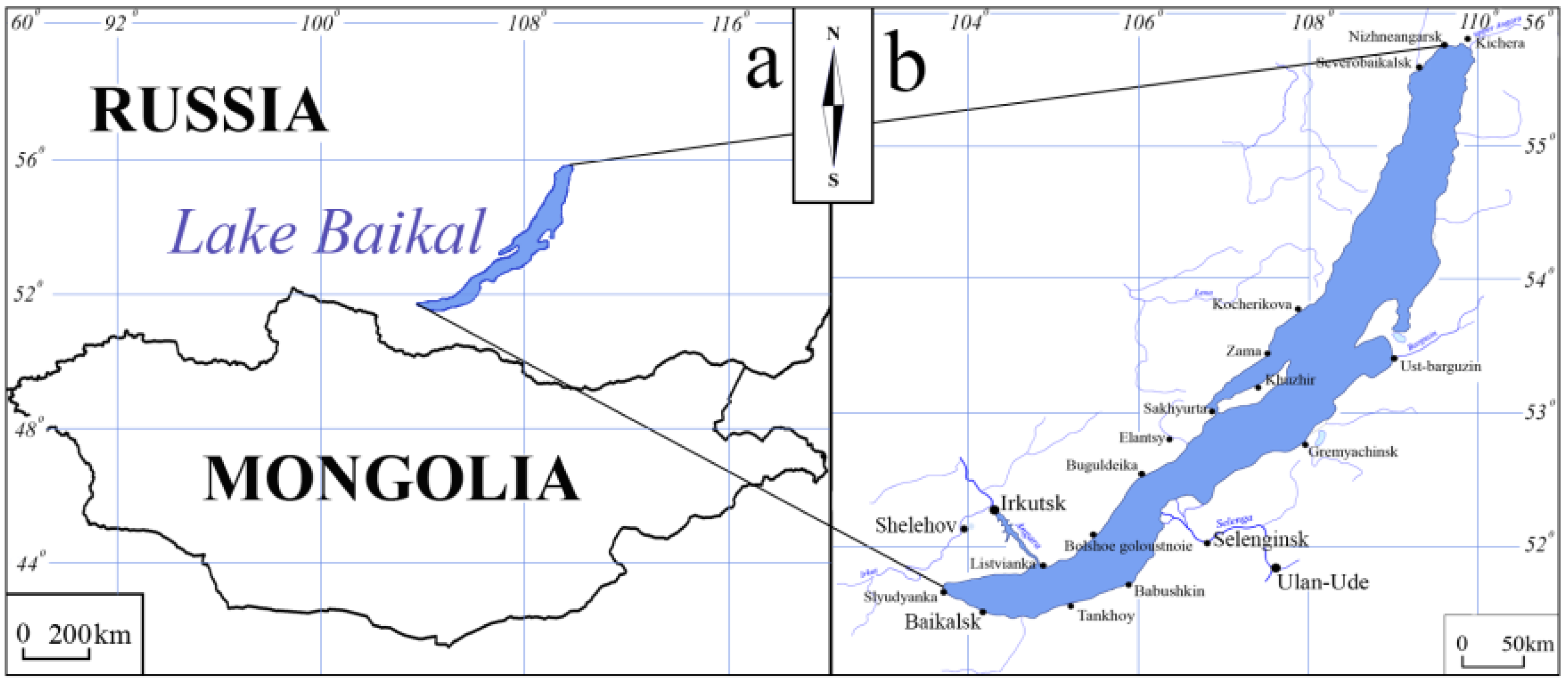
2.1. Study Area and Study Objects

The study was conducted at Lake Baikal (Figure 1) in June and February of 2015, 2018, 2019 and 2020. The study area is characterized by a continental climate and mountainous relief. The long, cold winters lasting from November to March and short hot summers lasting from June to August are typical for this area. Most of the precipitation falls during the period of positive air temperatures.

There are numerous PM sources located in the Lake Baikal area. Residential small-scale PM sources are located mostly on the lake shore [26]. Large-scale residential and industrial PM sources are located upwind from the lake along the Angara and Selenga River valleys [27].

The particulate matter (PM) in the air above the Lake Baikal and the PM accumulated in Lake Baikal snowpack were used as study objects. The choice of study objects was conditioned by the availability of data. Our previous studies were devoted to source apportionment of polycyclic aromatic hydrocarbons (PAH) and inorganic elements (IE) in airborne PM. To increase the performance of PMF model the old and the new datasets were united. The data on PAH concentrations in thirty-six samples of atmospheric PM collected in summer 2015 [26] were processed together with PAH data on 25 atmospheric PM samples collected in summer 2019 [28,29,30]. The data on IE concentrations in one hundred fifty-two snow samples collected in winter 2018 [13] and the data on IE concentrations in 47 samples collected in winter 2020 were also processed simultaneously. The missing data on some element concentrations in some locations were extracted from the literature [31,32,33,34].

The data on PAH composition of ambient air PM collected in summer and the data on IE composition of snow PM were processed independently, because the PAH sources are related to combustion processes, whereas the IE sources are related mostly to weathering and deterioration of anthropogenic materials. Moreover, the PAH sources (as well as IE sources) that contribute to air pollution in summer are mostly different from those that contribute to air pollution in winter.

2.2. Sampling Techniques

Atmospheric aerosol was sampled onboard the research vessel Akademik V.A. Koptyug according to the sampling scheme published previously by Golobokova et al. [28]. Airborne PM was collected on glass-fiber filters using a high-volume air sampler (Andersen Samplers Inc., Smyrna, GA, USA). The average volume of air drown through each filter was 45 m³.

The snow samples were taken from the lake ice surface in early March according to the sampling scheme published previously by Semenov et al. [13]. The snow height was within the range from several centimeters to tens of centimeters. Depending on snow height, snow was sampled using either snow coring tube or trowels.

2.3. Chemical Determinations

2.3.1. Polycyclic Aromatic Hydrocarbons

Sixteen PAHs were analyzed, including naphthalene (NAP), acenaphtene (ACE), fluorene (FLU), phenanthrene (PHE), anthracene (ANT), fluoranthene (FLA), pyrene (PYR), benzo[a]anthracene (BaA), chrysene (CHR), benzo[b]fluoranthene (BbF), benzo[k]fluoranthene (BkF), benzo[a]pyrene (BaP), benzo[e]pyrene (BeP), perylene (PER), benzo[g,h,i]perylene (BghiP), and indeno [1,2,3-c,d]pyrene (IcdP). Samples before extraction were spiked with PAH standard solutions. The samples were analyzed using an Agilent GC/MSD system equipped with DB-5 MS column. GC/MSD was calibrated prior to analysis to control the linearity of the responses. The selected ion monitoring mode was used for maximum sensitivity of MSD. PAHs were identified on the base of retention times of ion peaks. Quantification of identified PAHs was based on an internal standard method. The precision and the accuracy were good enough and ranged from 2% to 15%. The chemical determination of PAHs is described in more detail in Semenov et al., 2017 [26].

2.3.2. Inorganic Elements

Snow was melted, and the melt water was filtered through cellulose filters with a 0.45-micron pore size. Filters containing PM were dried. The element concentrations in PM were normalized to meltwater volume. Dry samples were digested using microwave acid digestion method. Teflon vessels were used for digestion of particulate matter samples in filters. Seven milliliters of concentrated HNO₃, 2 mL of concentrated HCl and 1 mL of concentrated HF were added to each vessel [35]. The digestion vessels were heated in the microwave oven according to selected digestion procedure. The digestate was diluted after digestion with deionized water before analysis.

The concentrations of Al, Si, Ba, V, Ti, Cr, Mn, Fe, Ni, Cu, Zn, Sr and Pb in digestate were measured using an Agilent 7500 ICP-MS. Samples were spiked with internal standard solutions. ICP-MS was calibrated prior to analysis to control the linearity of the responses. The multi-element standard solutions were used for calibration. Detection limits (DL) varied from 0.03 to 0.2 µg/L, depending on element measured. The precision and the accuracy ranged from 2 to 13%. The chemical determination of inorganic elements is described in more detail in Semenov et al., 2020 [13].

The element composition of leachate was also analyzed; however, the concentrations of soluble elements in snow meltwater was ten to one hundred times lower (depending on element) than the concentration of insoluble elements. This was probably due to the dissolution of readily soluble compounds that comprise fine PM during the snow melting and meltwater filtration processes. Since the concentrations of some elements in leachate were close to or below the detection limits, the combination of the data on soluble and insoluble element contents in PM would increase the uncertainty of PMF input data and decrease the quality of output data. Thus, only the data on the chemical composition of insoluble and poorly soluble PM was further used as input data for PMF analysis.

2.4. Data Processing

2.4.1. Data Analysis Using Positive Matrix Factorization Model

The source apportionment was performed using the EPA PMF 5 software package based on the data on PM chemistry. PMF decomposes the initial data matrix into a source profiles matrix and a source contributions matrix [36]:

X = G · F + E,

(1)

where X is the matrix of the input data, G is a matrix of the source contributions, F is a matrix of the source profiles, and E is the matrix of residuals (X − (G × F)).

The PMF objective is to reduce the squared standardized residuals or Q: the lower the Q, the lower the difference between real and modeled species concentrations. Before using the PMF model, the uncertainty of the measured data was evaluated. Uncertainties related to chemical measurements were taken into account by adding the values of one-third of DL to the measured uncertainty [37]. An additional 10% uncertainty was added to take into account the other possible errors [38]. Two datasets were analyzed separately, as the sources affecting two study objects could be different. Three to ten factors were run to identify the sources. The physical interpretability was used as the criterion of reliability of source profile [39]. To correct the PMF results the program parameter called F_peak was used. The source apportionment using PMF is described in more detail in Semenov et al., 2021 [25].

2.4.2. Testing the PMF Results Using Diagnostic Ratios and End-Member Mixing Analysis

The chemical species that can be used for calculation of source diagnostic ratios were selected from PMF-derived source profiles. The eligible species had to meet two criteria: (1) species concentrations in study object had to be high enough; (2) species concentrations had to be different in different source emissions. Since the EMMA approach considers the chemical composition of the study object as a mixture of chemical compositions of multiple source emissions, the obtained DR values were used as variable coefficients in simultaneous equations for calculation of source contributions:

$$\left\{\begin{array}{c}{\mathrm{f}}_1 + {\mathrm{f}}_2 + \cdots \dots \dots \dots + {\mathrm{f}}_{\mathrm{n}} = 1\\ {\mathrm{DR}}_1^1·{\mathrm{f}}_1 + {\mathrm{DR}}_2^1·{\mathrm{f}}_2 + .\dots \dots + {\mathrm{DR}}_{\mathrm{n}}^1·{\mathrm{f}}_{\mathrm{n}} = {\mathrm{DR}}_{\mathrm{mix}}^1\\ {\mathrm{DR}}_1^2·{\mathrm{f}}_1 + {\mathrm{DR}}_2^2·{\mathrm{f}}_2 + \dots \dots + {\mathrm{DR}}_{\mathrm{n}}^2·{\mathrm{f}}_{\mathrm{n}} = {\mathrm{DR}}_{\mathrm{mix}}^2\\ \dots \dots \dots .\dots \dots \dots \dots \dots \dots \dots \dots \dots \dots \dots \dots \dots \\ {\mathrm{DR}}_1^{\mathrm{m}}·{\mathrm{f}}_1 + {\mathrm{DR}}_2^{\mathrm{m}}·{\mathrm{f}}_2 + .\dots . + {\mathrm{DR}}_{\mathrm{n}}^{\mathrm{m}}·{\mathrm{f}}_{\mathrm{n}} = {\mathrm{DR}}_{\mathrm{mix}}^{\mathrm{m}}\end{array}\right.$$

(2)

where DR is a diagnostic ratio and f is the source contribution. Superscripts indicate the DR number, subscripts indicate the source number, and the subscript mix indicates study object or mixture.

If all the sources and source DRs have been selected properly, most of the obtained source contributions will meet three criteria: (1) contribution values will be positive; (2) contribution values will be less than 1, (3) the sum of source contributions calculated for each sample will be equal to 1.

Another way to verify whether the sources and source DRs have been selected properly is to draw the mixing diagrams. In this case, the DR values calculated on the base of each PMF-derived source profile are used as coordinates of source points in the EMMA mixing diagrams. The source points form a geometric shape called a mixing space, which bounds the sample points. The quality of PMF-derived source profiles is judged by the percentage of sample points bounded by profile-derived source points or by the position of the mixing space relative to the cloud of data points. When the sample points are inside the mixing space, all the sources contributed to sample pollution. The profiles of the sources whose uses result in the smallest number of sample points being inside the mixing space are considered to be unreliable. When the mixing spaces are inside the clouds of sample points, the profiles of sources whose uses result in the position of the mixing space being outside the data cloud are considered to be unreliable. If a sample point is outside the mixing space, only three neighboring sources (vertices of triangle face of tetrahedron) contributed to the pollution of that sample. Source contributions to a sample are inversely proportional to the distances between the projection of the sample point onto triangle and its vertices (source points). This graphical way of representing the EMMA results is the most illustrative. Unfortunately, it is impossible to graphically visualize the mixture of PM from more than four sources. Since the number of coordinate axes (DRs) must be one less than the number of sources, in order to visualize the mixture of PM from five sources, a four-dimensional coordinate system would be necessary.

3. Results and Discussion

3.1. Chemical Composition of Particulate Matter

3.1.1. PAH Composition of Particulate Matter

The obtained results showed that the PAH composition of airborne PM was highly variable among sampling sites. However, it was observed that PAH concentrations decreased in a direction towards the center of the lake. PAH concentrations also decreased with distance from settlements. The concentrations of PAH isomer pairs (PHE+ANT, FLA+PYR, BaA+CHR, BbF+BkF, BeP+BaP, IcdP+BghiP) decreased with increasing molecular weight (

Table 1. Basic statistical parameters of chemical composition of airborne particulate matter, ng/m³.

	NAP	ACE	FLU	PHE	ANT	FLA	PYR	BaA	CHR	BbF	BkF	BeP	BaP	PER	IcdP	BghiP
Min	0.01	0.001	0.003	0.01	0.001	0.01	0.01	3 × 10−4	0.003	0.01	0.001	2 × 10−5	1 × 10−5	1 × 10−5	3 × 10−5	2 × 10−5
25th *	0.02	0.01	0.01	0.04	0.002	0.03	0.02	0.001	0.01	0.02	0.01	4 × 10−5	2 × 10−5	1 × 10−5	1 × 10−5	1 × 10−5
Med	0.03	0.02	0.02	0.07	0.003	0.05	0.08	0.01	0.02	0.03	0.01	0.009	0.01	0.001	0.01	0.01
75th *	0.16	0.03	0.03	0.12	0.01	0.12	0.16	0.02	0.07	0.11	0.07	0.07	0.05	0.004	0.09	0.09
Max	34.9	10.9	14	36.4	0.03	7.57	10.3	1.57	6.91	14.1	5.09	0.48	0.2	0.02	0.36	0.33
Mean	0.74	0.14	0.18	0.48	0.01	0.19	0.35	0.03	0.16	0.27	0.10	0.06	0.03	0.01	0.06	0.06
STD **	4.19	1.12	1.43	3.73	0.01	0.78	1.33	0.16	0.77	1.45	0.52	0.11	0.05	0.01	0.09	0.08

* percentile, ** standard deviation.

). The highest and the lowest mean concentrations were observed for NAP and PER, respectively. The high concentrations of low-molecular-weight (LMW) PAHs such as NAP, ACE, FLU, PHE and ANT were due to their high volatility and solubility. The highest standard deviations were observed for NAP and PHE and the lowest STD values were observed for BaP and PER.

3.1.2. Element Composition of Particulate Matter

As in the case of PAHs, the elemental composition of snow PM varied significantly. Similar to PAH concentrations, the element concentrations decreased in a direction towards the center of the lake. Concentrations of inorganic elements also decreased with increasing distance from settlements. The concentrations of V, Ni, Cu, Cr, Ti, and Pb were very low, and the concentrations of Si, Al, Fe, Zn, Mn, Ba and Sr were high (

Table 2. Basic statistical parameters of chemical composition of insoluble particulate matter in snow meltwater, µg/L.

Parameter	Al	Si	Ba	V	Ti	Cr	Mn	Fe	Ni	Cu	Zn	Sr	Pb
Min	0.77	1.97	0.45	0.25	0.41	0.56	0.56	0.88	0.34	0.42	0.62	0.82	0.20
25th *	6.21	1.35	2.32	1.12	1.23	1.04	3.42	3.32	1.01	1.22	0.98	3.20	1.05
Median	12.2	6.06	3.21	1.44	1.05	1.13	6.23	6.45	1.31	1.97	2.43	6.22	1.14
75th *	21.0	80.1	5.55	1.99	2.39	1.87	10.3	14.1	1.12	3.44	7.18	12.4	1.25
Max	97.6	2107	62.4	7.01	10.7	26.6	54.9	70.2	8.37	9.31	26.3	98.7	10.9
Mean	18.0	88.2	4.13	1.60	1.55	1.74	8.21	11.6	1.27	2.30	4.69	10.4	1.47
STD **	18.4	252	5.63	1.19	1.41	2.48	8.86	14.5	0.70	1.60	5.31	13.1	1.32

* percentile, ** standard deviation.

). The highest and the lowest mean concentrations were observed for Si and Ni, respectively. The highest standard deviations were observed for Si and Al and the lowest STD values were observed for Ni and V.

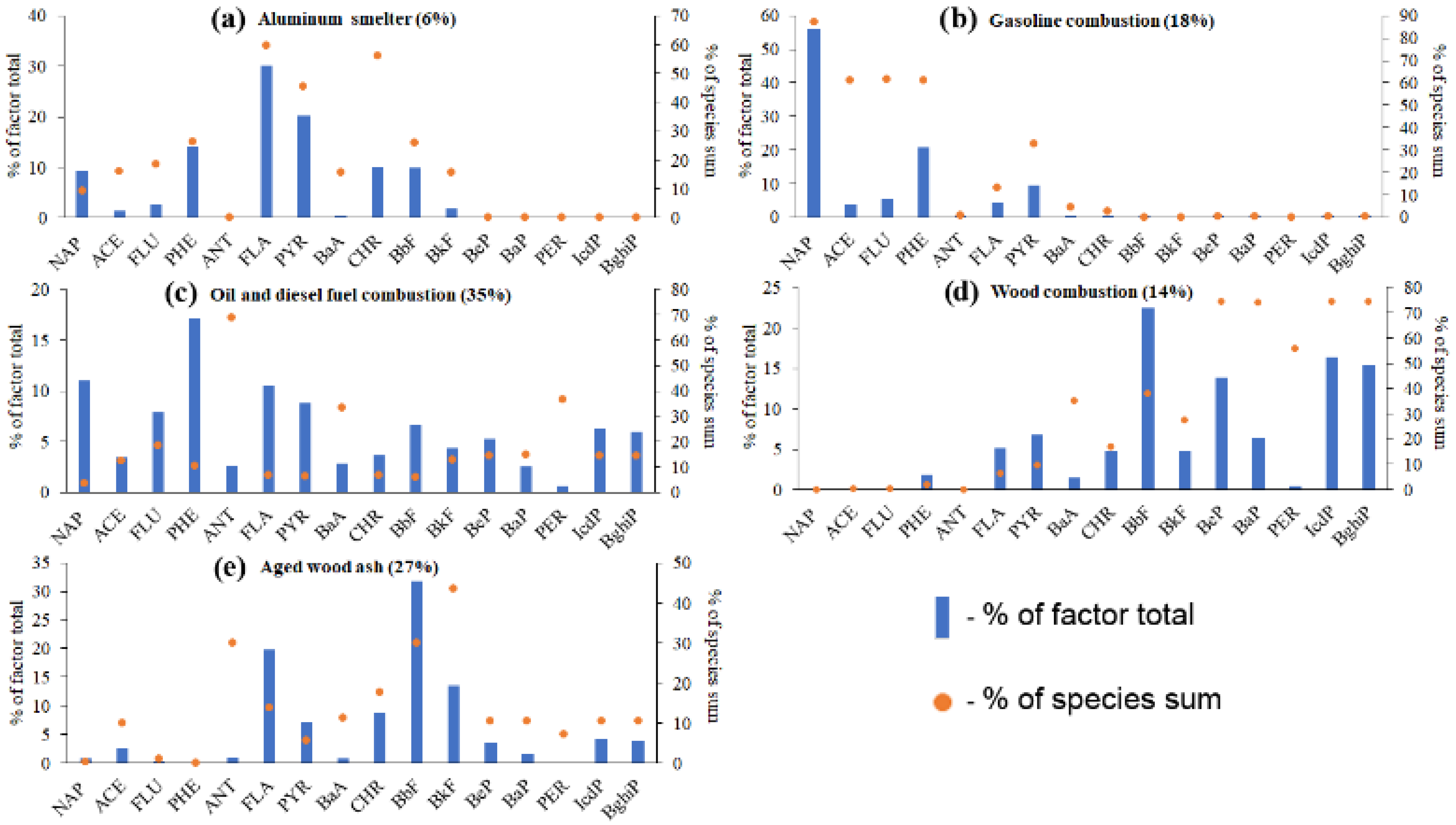
3.2. Resolving the PAH Profiles of PM Sources in the Air above the Lake Baikal Water Using PMF

The rotated (F_peak = 0.5) five-factor solution was the most interpretable result obtained for PAH sources in atmospheric particulate matter. Those factors contributed 6%, 18%, 35%, 14% and 27% of PAHs to PM, respectively (Figure 2). The differences between Q_true and Q_expected were less than 16%.

Factor 1 (Figure 2a) was characterized by the relatively high concentrations of fluoranthene and pyrene. The factor’s contributions to concentrations of these PAHs were equal to 30% and 20%, respectively. The predominance of FLU and PYR is typical for emissions of paper mills and aluminum smelters [40]. Nevertheless, it was supposed that this factor represented the aluminum smelter, because the obtained PAH composition was quite similar to that of grass and soil sampled in the vicinity of aluminum smelter [41] except the concentrations of BaP, IcdP and BghiP (Figure 3a). The contribution of Factor 1 to concentrations of BeP, BaP, PER, IcdP and BghiP was lowest among the other factors.

Factor 2 (Figure 2b) was characterized by the highest concentration of NAP among all factors. The concentration of NAP absolutely prevailed over the other PAHs. This factor was also characterized by the highest contribution to concentrations of NAP, ACE, FLU and PHE. It was supposed that this factor represented gasoline combustion, because the prevalence of LMW PAHs over HMW PAHs (BaA, CHR, BbF, BkF, BeP, BaP, PER, IcdP, BghiP) is the characteristic feature of combustion of unsaturated light-weight cyclic hydrocarbons [42]. Finally, the obtained profile was quite similar to that of gasoline combustion reported by Mi et al. [42] (Figure 3b).

The Factor 3 (Figure 2c) profile was also characterized by the prevalence of LMW PAHs over HMW PAHs; however, the LMW/HMW ratio in Factor 3 was much lower than that in Factor 2. This was probably due to the higher concentration of HMW PAHs in burned fuel. Diesel oil could be such a fuel. However, the diesel oil combustion profiles presented in the literature [43] are characterized by higher LMW/HMW ratio (Figure 3c) than that in Factor 3. Thus, it was supposed that HMW PAHs in Factor 3 originated from both combustion of diesel fuel and combustion of heavy petroleum fractions.

The PAH emission profiles of Factor 4 (Figure 2d) and Factor 5 (Figure 2e) were quite similar. Both factors were characterized by the dominance of HMW PAHs over LMW PAHs. Another feature of the two profiles was the dominance of BbF over the other PAHs. Nevertheless, the PAH emission compositions of these sources are similar to that of wood combustion [44], which is characterized by the dominance of BaA and IcdP (Figure 3d). Since the profile of Factor 4 was most similar to that of wood combustion reported by Li et al. [44], it was ascribed to wood combustion. Factor 5 was ascribed to aged wood ash, because it has increased BbF and BkF and decreased IcdP and BghiP with respect to Factor 4. The enrichment of BbF and BkF in Factor 5 was due to their resistance to oxidation [45], especially in the darkness [46]. The depletion of IcdP and BgiP in Factor 5 was due to their selective oxidation by NOx and O₃. The enrichment of FLA in Factor 5 was probably due to adsorption of gaseous fluoranthene onto aerosol particle surfaces. The obtained profiles of wood combustion and aged wood ash were characterized by a higher portion of HMW PAHs than those of gasoline and diesel oil combustion. This fact contradicts the results of some studies claiming that HMW PAHs are formed during high-temperature processes like fuel combustion in engines, whereas LMW PAHs are usually formed during low-temperature processes like wood combustion [23,47]. This contradiction was probably due to the fact that PAH source signatures reflect the unique combination of fuel origin, industrial production intensity, equipment manufacturer, and degree of equipment deterioration [26]. In other words, PAH isomer ratios may show substantial intra-source variability and inter-source similarity [48].

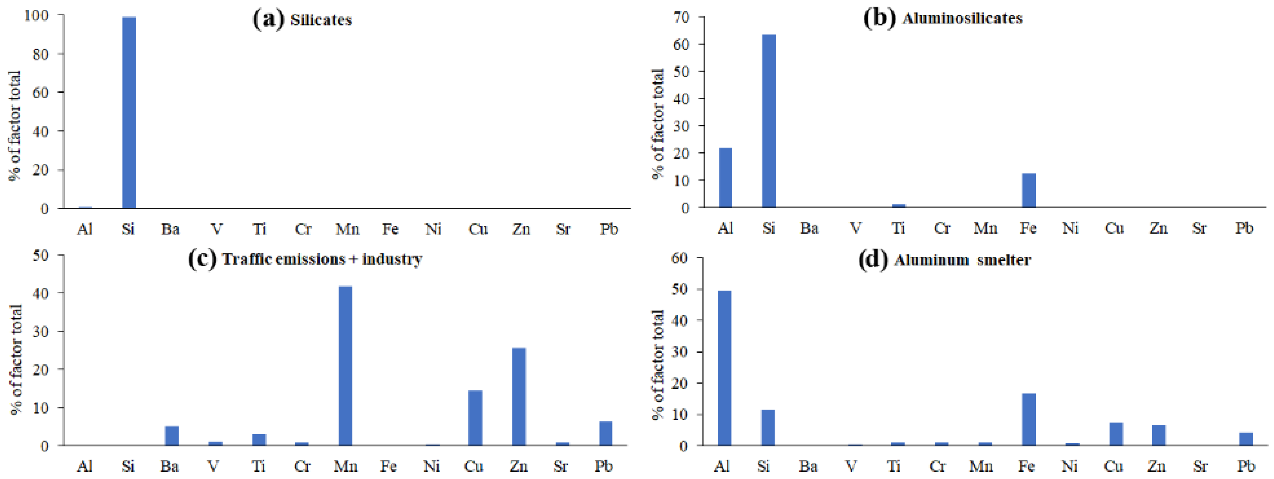
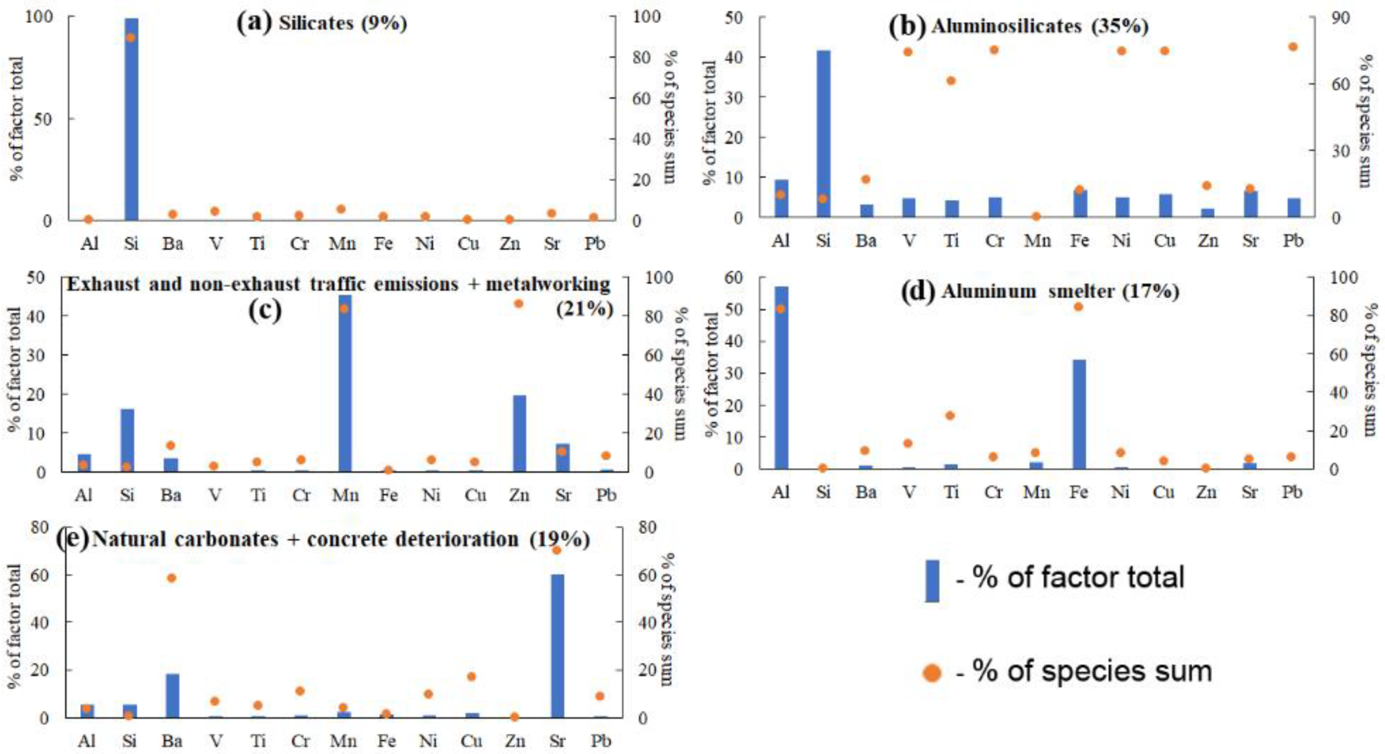
3.3. Resolving the IE Profiles of PM Sources in the Lake Baikal Snowpack Using PMF

The five-factor PMF solution was obtained for inorganic pollutant sources in Lake Baikal snowpack. The solution was stable (Q_true/Q_expected = 1.2) and the factor mass fractions did not change with varying F_peak. The obtained factors contributed 9%, 35%, 17%, 21% and 19% of inorganic elements to PM, respectively (Figure 4). In contrast to the PMF-derived PAH profiles, the IE profiles were characterized by a low number of chemical species that could be used for calculating the source diagnostic ratios (Figure 4).

Factor 1 (Figure 4a) was characterized by the extremely high concentration of Si (98%) and by the extremely high contribution to Si concentrations (95%) in snow-deposited PM samples. This factor was attributed to silicates, which are ubiquitous components of natural and anthropogenic aerosols [49]. The obtained profile was quite similar to those of quartz sands reported by Štyriaková et al. (2009) [50] and by Rokbi and Baali [51] (Figure 5a).

Factor 2 (Figure 4b) was also characterized by high Si concentration; however, it was attributed to aluminosilicates, because the Si/Al ratio was equal to 3.8, which is typical for aluminosilicates [25]. The obtained profile of aluminosilicates matched that obtained previously for PM derived from urban snowpack in Irkutsk city [25]. The obtained composition of aluminosilicates was also in agreement with the existing knowledge of aluminosilicates chemistry [52] (Figure 5b). Unlike Factor 1, the contribution of Factor 2 to the concentration of Si was quite small, whereas its contribution to the concentrations of trace elements was very high. The high contribution of Factor 2 to concentrations of heavy metals was probably due to metal sorption by some aluminosilicate minerals such as clays. It is noteworthy that the sum of abundances of silicates (Factor 1) and aluminosilicates (Factor 2) matched the abundance of soil-dust in airborne PM over Lake Baikal reported by Van Malderen et al. [53].

Factor 3 (Figure 4c) was characterized by the highest concentration of Mn, as well as by the highest contribution to Mn concentration among all factors. This probably indicates the influence of both exhaust traffic emissions and metalworking. It is known that methylcyclopentadienyl manganese tricarbonyl (MMT) is usually added to unleaded gasoline to increase the octane rating [54]. The combustion of unleaded gasoline along with steel treatment may result in contamination of air by Mn in urban environments [55,56]. The element composition of Factor 3 (except the Al and Si) was similar to that of PM sampled in heavy traffic sites in industrial cities reported by Amato et al. [57] (Figure 5c). The presence of Al and Si (which are the major constituents of road pavements and curbs) in Factor 3 probably testifies to the fact that a minor part of PM associated with this factor was originated from non-exhaust traffic emissions. There are numerous cities and settlements are located on lake shores; thus, snow pollution by Mn, Al and Si from local sources is quite possible. The pollution of Lake Baikal snowpack by these elements from remote sources also seems probable, because large industrial centers are located upwind from the lake along the Angara (cities Shelekhov, Angarsk and Irkutsk) and Selenga (cities Gusinoosersk, Selenginsk and Ulan-Ude) river valleys [27].

The pollutant transport from remote sources may also explain the chemical composition of Factor 4 (Figure 4d) characterized by high concentrations of Al and Fe. The enrichment of PM with Al and Fe is characteristic for emissions from aluminum smelters. The element composition of Factor 4 matched those of PM derived from snow, soil, and air in the vicinity of aluminum smelters [58,59] (Figure 5d).

Factor 5 (Figure 4e) was ascribed to the degradation of calcium-rich materials such as carbonate rocks and concrete, because the particulate matter associated with Factor 5 was enriched with Sr and Ba. Being the geochemical analogues of calcium, Sr and Ba isomorphically substitute Ca in most minerals, especially in carbonates. Thus, the concentrations of Ca, Sr and Ba are always proportional to each other. Unfortunately, the calcium concentrations in PM samples were not taken into consideration in this study because of the low accuracy of the Ca measurement.

Figure 5. Source profiles derived from the literature: (a) average IE composition of silicates reported by Štyriaková et al. [50] and Rokbi and Baali [51], (b) IE composition of aluminosilicates reported by Bleam [52], (c) IE composition of traffic and industrial emissions reported by Amato et al. [57], (d) average IE composition of snow, soil, and air PM in the vicinity of aluminum smelter reported by Boullemant [58] and Belozertseva [59].

Figure 5. Source profiles derived from the literature: (a) average IE composition of silicates reported by Štyriaková et al. [50] and Rokbi and Baali [51], (b) IE composition of aluminosilicates reported by Bleam [52], (c) IE composition of traffic and industrial emissions reported by Amato et al. [57], (d) average IE composition of snow, soil, and air PM in the vicinity of aluminum smelter reported by Boullemant [58] and Belozertseva [59].

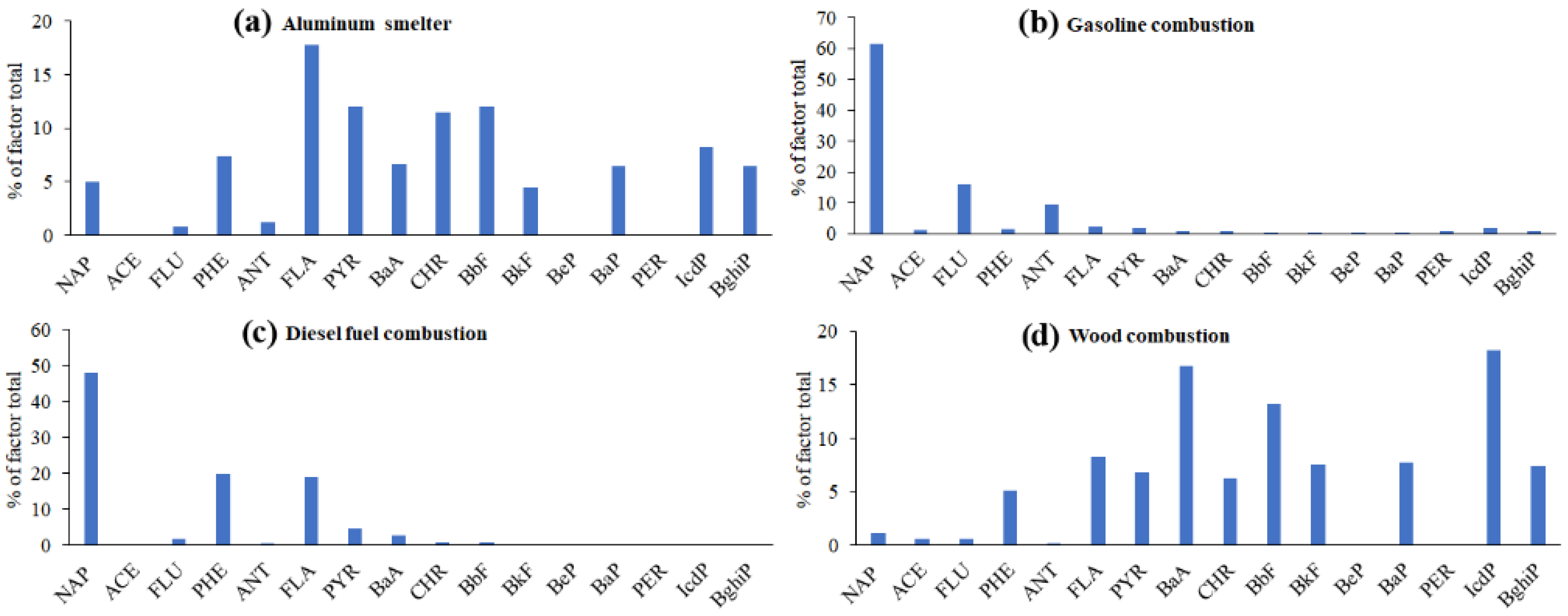
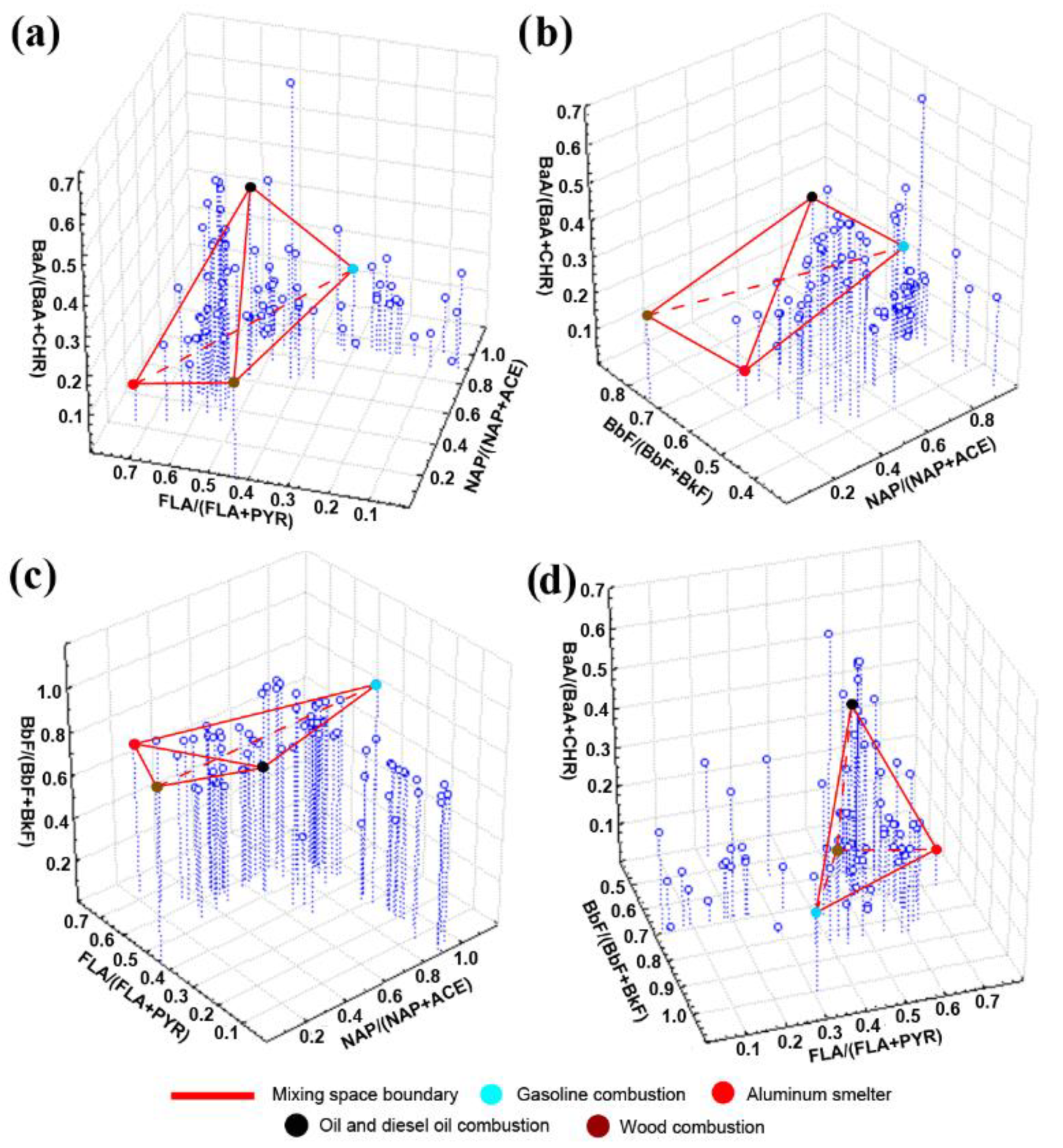
3.4. Testing the PMF-Derived Source Profiles of Airborne PAHs Using EMMA and DR

Based on Figure 2, four PAH isomer pairs characterized by distinctly different concentrations of isomers (

Table 3. PMF-derived PAH diagnostic ratios.

	NAP/(NAP+ACE)	FLA/(FLA+PYR)	BaA/(BaA+CHR)	BbF/(BbF+BkF)
Gasoline combustion	0.94	0.31	0.20	1.00
Aluminum smelter	0.24	0.74	0.09	0.70
Oil combustion	0.76	0.54	0.44	0.61
Wood combustion	0.01	0.43	0.24	0.82
Aged wood ash	0.25	0.71	0.18	0.71

) were selected as being eligible for calculating diagnostic ratios to distinguish PM emission sources. First of all, simultaneous equations were solved for five PMF-derived PAH sources using four source tracers. However, the source contributions calculated for most of the samples (97%) were negative. This meant that the number of major sources was less than five.

Since the number of source tracers must be one less than the number of sources, the three most suitable source DRs had to be selected to apportion the four most suitable PAH sources. To identify tracers and sources, all possible pseudo-3D mixing diagrams that use the obtained DR ratios as coordinates of source points were generated (Figure 6).

It was found that the position of the point of aged wood ash in any coordinate system matched the position of some other source (mostly the positions of aluminum smelter and wood combustion). Thus, aged wood ash was recognized as a minor source. As can be clearly seen from Figure 6, mixing tetrahedrons formed by gasoline combustion, aluminum smelter, oil combustion and wood combustion bounded at least one-third of PM samples (Figure 6b). This means that the PMF-derived profiles of those four sources are valid to a great extent. It must be taken into account that the difference between the sample points inside and outside the mixing space is only in the number of sources that contribute to pollution of corresponding sample. The highest proportion of sample points fell within the mixing space formed by PM sources using values of FLA/(FLA+PYR) and BaA/(BaA+CHR) ratios as coordinates (Figure 6a,d). The lowest proportion of sample points fell within the mixing space formed by PM sources using NAP/(NAP+ACE) and BbF/(BbF+BkF) ratios as coordinates (Figure 6b,c). The greater applicability of FLA/(FLA+PYR) and BaA/(BaA+CHR) ratios with respect to NAP/(NAP+ACE) and BbF/(BbF+BkF) ratios for source apportionment of PAHs was probably due to the similar molecular weights of FLA, PYR, BaA and CHR. Similar molecular weights cause similar chemical properties and, consequently, similar degradation rates; thus, the source fingerprints do not change drastically over time.

The contributions of respective sources to the PAH composition of PM obtained using four sets of tracers were very different (

Table 4. Contributions of PM sources to airborne PAHs calculated using different tracers, %.

Source/Tracer	NAP/(NAP+ACE)	NAP/(NAP+ACE)	NAP/(NAP+ACE)	FLA/(FLA+PYR)
	FLA/(FLA+PYR)	BbF/(BbF+BkF)	FLA/(FLA+PYR)	BbF/(BbF+BkF)
	BaA/(BaA+CHR)	BaA/(BaA+CHR)	BbF/(BbF+BkF)	BaA/(BaA+CHR)
Gasoline combustion	32	27	20	23
Aluminum smelter	39	37	38	49
Oil and diesel fuel combustion	22	32	37	11
Wood combustion	6	3	5	17

). The greatest differences between source contributions obtained using PMF model and EMMA (on the base of PMF-derived DRs) were observed for aluminum smelter and wood combustion, whereas the lowest differences were observed for gasoline combustion and oil/diesel fuel combustion.

3.5. Testing the PMF-Derived Source Profiles of Airborne Inorganic PM Using EMMA and DR

Based on Figure 4, three element concentration ratios (

Table 5. PMF-derived element diagnostic ratios.

	Al/(Al+Si)	Mn/(Mn+Fe)	Ba/(Ba+Sr)
Silicates	0.01	0.66	0.25
Aluminasilicates	0.18	0.02	0.35
Traffic emissions + metalworking	0.22	0.99	0.33
Aluminum smelter	1.00	0.06	0.42
Natural carbonates + concrete deterioration	0.50	0.63	0.24
Average	0.38	0.47	0.32

) were selected as being eligible for calculating diagnostic ratios. Thus, four major PM emission sources had to be identified. To identify these sources, all possible pseudo-3D mixing diagrams that used the obtained DR ratios as coordinates of source points were generated (Figure 7).

The highest proportion of sample points fell within the mixing space formed by aluminum smelter, aluminosilicates, silicates, exhaust and non-exhaust traffic emissions + metalworking (Figure 7c). None of the possible combinations of natural carbonates and concrete with the any other three PM sources (Figure 7a,b,d) made it possible to bound more than one-tenth of the sample points. This was probably due to the fact that the values of Al/(Al+Si), Mn/(Mn+Fe) and Ba/(Ba+Sr) ratios characteristic for natural carbonates and concrete were close to the average values of respective ratios calculated for all the four PM sources (Table 5). Thus, the PMF-derived source of Ca-Sr-Ba-rich particulate matter identified as “natural carbonates and concrete deterioration” is probably a minor source which does not significantly affect the chemical composition of snow PM. Additionally, this source may not exist at all. On the contrary, the PMF-derived profiles of the remaining four sources can be considered to be major ones.

As can be clearly seen from

Table 6. Contributions of PM sources to airborne IEs calculated using Al/(Al+Si), Mn/(Mn+Fe) and Ba/(Ba+Sr) ratios as tracers, %.

Source	Contribution
Silicates	33
Aluminosilicates	27
Traffic emissions + metalworking	13
Aluminum smelter	26

, the contributions of respective sources obtained using EMMA and the PMF model (Figure 4) were different.

This was expected, because the methods used for calculations were also different. The greatest difference (24%) between source contributions obtained using PMF model and EMMA was observed for silicates. The difference between contributions of any of the other three sources obtained using PMF model and EMMA was 8–9%.

4. Conclusions

This study was the first attempt to test the PMF results using source apportionment techniques that are not based on multivariate analysis; thus, the obtained results are not exhaustive. Nevertheless, it can be said with certainty that the validation of PMF-derived source profiles using EMMA compensates for the uncertainty related to the number of factors that should be retained in PMF analysis. The main conclusions reached in this study are as follows:

• Emission profiles of four of the five PAH sources obtained using PMF were quite reliable, because the mixing spaces in EMMA diagrams that used PMF-derived DR ratios as coordinates of PAH source points bounded 25–75% of airborne PM samples. The aged wood ash was recognized as the minor source because its point in any coordinate system matched the position of some other sources (mostly the positions of aluminum smelter and wood combustion).
• The reliability of PMF-derived PAH source profiles was most evident in the mixing diagrams that used PAHs with similar molecular weights as tracers. Similar molecular weights caused similar chemical properties of the tracer PAHs and, consequently, similar degradation rates. Thus, the PAH source fingerprints did not change drastically over time.
• The reliability of the results of EMMA-DR testing of PMF-derived IE source profiles was controversial. On the one hand, the mixing spaces in most of the EMMA diagrams that used PMF-derived DR ratios as coordinates of IE source points did not bound more than one-tenth of the sample points. On the other hand, the mixing space formed by the PMF-derived sources except natural carbonates + concrete deterioration bounded most of the sample points. This probably means that the PMF-derived Ca-Sr-Ba-rich source identified as “natural carbonates + concrete deterioration” was a minor one, whereas the other sources were major ones.
• The identification of continuously operating PM sources (aluminum smelter and traffic emissions) using both organic and inorganic tracers also argues in favor of the reliability of PMF-derived PAH and IE source profiles.
• The PMF-derived PM source profiles whose reliability was not confirmed by EMMA-DR results should be considered unreliable. The contributions of validated PMF-derived sources should be normalized to 100% after removal of the contributions of unvalidated sources.
• To improve the reliability of the PMF results, the concentrations of alkali and alkaline-earth metals like Na, K, Mg and Ca should be included in PMF analysis.
• To increase the capability of EMMA-DR testing of PMF results more chemical species from PMF-derived source profiles should be included in the testing procedure as source tracers. To include more chemical species in EMMA-DR, the relevant Excel-based computational tools should be developed.

References

1. Thurston, G.D.; Ito, K.; Lall, R. A source apportionment of U.S. fine particulate matter air pollution. Atmos. Environ. 2011, 45, 3924–3936. [Google Scholar] [CrossRef] [PubMed] [Green Version]
2. Song, Y.; Xie, S.; Zhang, Y.; Zeng, L.; Salmon, L.G.; Zheng, M. Source apportionment of PM2.5 in Beijing using principal component analysis/absolute principal component scores and UNMIX. Sci. Total Environ. 2006, 372, 278–286. [Google Scholar] [CrossRef] [PubMed]
3. Beddows, D.C.S.; Dall’Osto, M.; Harrison, R.M. Cluster analysis of rural, urban and curbside 916 atmospheric particle size data. Environ. Sci. Technol. 2009, 43, 4694–4700. [Google Scholar] [CrossRef] [PubMed]
4. Chen, L.; Qi, X.; Nie, W.; Wang, J.; Xu, Z.; Wang, T.; Liu, Y.; Shen, Y.; Xu, Z.; Kokkonen, T.V.; et al. Cluster analysis of submicron particle number size distributions at the SORPES station in the Yangtze River Delta of East China. J. Geophys. Res. Atmos. 2021, 126, e2020JD034004. [Google Scholar] [CrossRef]
5. Wan, X.; Chen, J.; Tian, F.; Sun, W.; Yang, F.; Saiki, K. Source apportionment of PAHs in atmospheric particulates of Dalian: Factor analysis with nonnegative constraints and emission inventory analysis. Atmos. Environ. 2006, 40, 6666–6675. [Google Scholar] [CrossRef]
6. Hu, N.-J.; Huang, P.; Liu, J.-H.; Ma, D.-Y.; Shi, X.-F.; Mao, J.; Liu, Y. Characterization and source apportionment of polycyclic aromatic hydrocarbons (PAHs) in sediments in the Yellow River Estuary, China. Environ. Earth Sci. 2014, 71, 873–883. [Google Scholar] [CrossRef]
7. Larsen, R.K.; Baker, J. Source apportionment of polycyclic aromatic hydrocarbons in the urban atmosphere: A comparison of three methods. Environ. Sci. Technol. 2003, 37, 1873–1881. [Google Scholar] [CrossRef]
8. Cai, K.; Li, C. Street dust heavy metal pollution source apportionment and sustainable management in a typical City-Shijiazhuang, China. Int. J. Environ. Res. Public Health 2019, 16, 2625. [Google Scholar] [CrossRef] [Green Version]
9. Song, Y.; Li, H.; Li, J.; Mao, C.; Ji, J.; Yuan, X.; Li, T.; Ayoko, G.; Frost, R.L.; Feng, Y.-X. Multivariate linear regression model for source apportionment and health risk assessment of heavy metals from different environmental media. Ecotoxicol. Environ. Saf. 2018, 165, 555–563. [Google Scholar] [CrossRef]
10. Henry, R.C. Multivariate receptor modeling by N-dimensional edge detection. Chemom. Intell. Lab. Syst. 2003, 65, 179–189. [Google Scholar] [CrossRef]
11. Paatero, P.; Tapper, U. Positive matrix factorization: A non-negative factor model with optimal utilization of error estimates of data values. Environmetrics 1994, 5, 111–126. [Google Scholar] [CrossRef]
12. Semenov, M.Y.; Marinaite, I.I.; Bashenkhaeva, N.V.; Zhuchenko, N.A.; Khuriganova, O.I.; Molozhnikova, E.V. Polycyclic aromatic hydrocarbons in a small eastern Siberian river: Sources, delivery pathways, and behavior. Environ. Earth Sci. 2016, 75, 954. [Google Scholar] [CrossRef]
13. Semenov, M.Y.; Silaev, A.V.; Semenov, Y.M.; Begunova, L.A. Using Si, Al and Fe as tracers for source apportionment of air pollutants in Lake Baikal snowpack. Sustainability 2020, 12, 3392. [Google Scholar] [CrossRef] [Green Version]
14. Chen, L.W.A.; Lowenthal, D.H.; Watson, J.G.; Koracin, D.; Kumar, N.; Knipping, E.M.; Wheeler, N.; Craig, K.; Reid, S. Toward effective source apportionment using positive matrix factorization: Experiments with simulated PM 2.5 data. J. Air Waste Manag. Assoc. 2010, 60, 43–54. [Google Scholar] [CrossRef]
15. Brown, S.G.; Eberly, S.; Paatero, P.; Norris, G.A. Methods for estimating uncertainty in PMF solutions: Examples with ambient air and water quality data and guidance on reporting PMF results. Sci. Total Env. 2015, 518–519, 626–635. [Google Scholar] [CrossRef] [Green Version]
16. Viana, M.; Pandolfi, M.; Minguillón, M.C.; Querol, X.; Alastuey, A.; Monfort, E.; Celades, I. Inter-comparison of receptor models for PM source apportionment: Case study in an industrial area. Atmos. Environ. 2008, 42, 3820–3832. [Google Scholar] [CrossRef]
17. Shi, G.L.; Liu, G.R.; Peng, X.; Wang, Y.N.; Tian, Y.Z.; Wang, W.; Feng, Y.C. A comparison of multiple combined models for source apportionment, including the PCA/MLR-CMB, Unmix-CMB and PMF-CMB Models. Aerosol Air Qual. Res. 2014, 14, 2040–2050. [Google Scholar] [CrossRef] [Green Version]
18. Salim, I.; Sajjad, R.U.; Paule-Mercado, M.C.; Memon, S.A.; Lee, B.Y.; Sukhbaatar, C.; Lee, C.H. Comparison of two receptor models PCA-MLR and PMF for source identification and apportionment of pollution carried by runoff from catchment and sub-watershed areas with mixed land cover in South Korea. Sci. Total Environ. 2019, 663, 764–775. [Google Scholar] [CrossRef]
19. Feng, J.; Song, N.; Yu, Y.; Li, Y. Differential analysis of FA-NNC, PCA-MLR, and PMF methods applied in source apportionment of PAHs in street dust. Environ. Monit. Assess. 2020, 192, 727. [Google Scholar] [CrossRef]
20. Zanotti, C.; Rotiroti, M.; Fumagalli, L.; Stefania, G.A.; Canonaco, F.; Stefenelli, G.; Prévôt, A.S.H.; Leoni, B.; Bonomi, T. Groundwater and surface water quality characterization through positive matrix factorization combined with GIS approach. Water Res. 2019, 159, 122–134. [Google Scholar] [CrossRef]
21. Souto-Oliveira, C.E.; Kamigauti, L.Y.; Andrade, M.d.F.; Babinski, M. Improving source apportionment of urban aerosol using multi-isotopic fingerprints (MIF) and positive matrix factorization (PMF): Cross-validation and new insights. Front. Environ. Sci. 2021, 9, 623915. [Google Scholar] [CrossRef]
22. Wen, Z.; Li, B.; Xiao, H.Y.; Zhe, L.; Zhu, R.G. Combined positive matrix factorization (PMF) and nitrogen isotope signature analysis to provide insights into the source contribution to aerosol free amino acids. Atmos. Environ. 2022, 268, 118799. [Google Scholar] [CrossRef]
23. Tobiszewski, M.; Namiesnik, J. PAH diagnostic ratios for the identification of pollution emission sources. Environ. Pollut. 2012, 162, 110–119. [Google Scholar] [CrossRef] [PubMed]
24. Christophersen, N.; Neal, C.; Hooper, R.P.; Vogt, R.D.; Andersen, S. Modelling streamwater chemistry as a mixture of soilwater end-members—A step towards second-generation acidification models. J. Hydrol. 1990, 116, 307–320. [Google Scholar] [CrossRef]
25. Semenov, M.Y.; Onishchuk, N.A.; Netsvetaeva, O.G.; Khodzher, T.V. Source apportionment of particulate matter in urban snowpack using end-member mixing analysis and positive matrix factorization model. Sustainability 2021, 13, 13584. [Google Scholar] [CrossRef]
26. Semenov, M.Y.; Marinaite, I.I.; Golobokova, L.P.; Khuriganova, O.I.; Khodzher, T.V.; Semenov, Y.M. Source apportionment of polycyclic aromatic hydrocarbons in Lake Baikal water and adjacent air layer. Chem. Ecol. 2017, 33, 977–990. [Google Scholar] [CrossRef]
27. Obolkin, V.A.; Potemkin, V.L.; Makukhin, V.L.; Khodzher, T.V.; Chipanina, E.V. Long-range transport of plumes of atmospheric emissions from regional coal power plants to the South Baikal water basin. Atmos. Ocean. Opt. 2017, 30, 360–365. [Google Scholar] [CrossRef]
28. Golobokova, L.; Khodzher, T.; Khuriganova, O.; Marinayte, I.; Onishchuk, N.; Rusanova, P.; Potemkin, V. Variability of chemical properties of the atmospheric aerosol above Lake Baikal during large wildfires in Siberia. Atmosphere 2020, 11, 1230. [Google Scholar] [CrossRef]
29. Marinaite, I.I.; Potyomkin, V.L.; Khodzher, T.V. Evaluation of atmospheric pollution with PAHS and PM10 above the water area of Lake Baikal during wildfires in Summer. In Proceedings of the 26th International Symposium on Atmospheric and Ocean Optics, Atmospheric Physics, Moscow, Russia, 6–10 July 2020; Volume 115602. [Google Scholar] [CrossRef]
30. Marinaite, I.I.; Potyomkin, V.L.; Molozhnikova, E.V.; Penner, I.E.; Shikhovtsev, M.Y.; Izosimova, O.N.; Khodzher, T.V. Polycyclic aromatic hydrocarbons and PM10 solid particles above the water area of Lake Baikal in the summer of 2020. In Proceedings of the 27th International Symposium on Atmospheric and Ocean Optics, Atmospheric Physics, Moscow, Russia, 5–9 July 2021; Volume 119161. [Google Scholar] [CrossRef]
31. Belozertseva, I.A.; Vorobyeva, I.B.; Vlasova, N.V.; Lopatina, D.N.; Yanchuk, M.S. Snow pollution in Lake Baikal water area in nearby land areas. Water Resour. 2017, 44, 471–484. [Google Scholar] [CrossRef]
32. Belozertseva, I.A.; Vorobyeva, I.B.; Vlasova, N.V.; Janchuk, M.S.; Lopatina, D.N. Chemical composition of snow water of the water area of the southern hollow of Lake Baikal. Int. J. Appl. Fundam. Res. 2016, 10, 263–272. (In Russian) [Google Scholar]
33. Belozertseva, I.A.; Vorobeva, I.B.; Vlasova, N.V.; Yanchuk, M.S.; Lopatina, D.N. Pollution of snow on the water area of the average hollow of Lake Baikal and the adjacent territory. Adv. Curr. Nat. Sci. 2016, 11, 96–105. (In Russian) [Google Scholar]
34. Belozertseva, I.A.; Vorobeva, I.B.; Vlasova, N.V.; Yanchuk, M.S.; Lopatina, D.N. Pollution of snow on the water area of the northern hollow of Lake Baikal and the adjacent territory. Adv. Curr. Nat. Sci. 2016, 9, 97–103. (In Russian) [Google Scholar]
35. Liang, S.X.; Wu, H.; Sun, H.W. Determination of trace elements in airborne PM10 by inductively coupled plasma mass spectrometry. Int. J. Environ. Sci. Technol. 2015, 12, 1373–1378. [Google Scholar] [CrossRef] [Green Version]
36. Lucarelli, F.; Calzolai, G.; Chiari, M.; Giardi, F.; Czelusniak, C.; Nava, S. Hourly elemental composition and source identification by positive matrix factorization (PMF) of fine and coarse particulate matter in the high polluted industrial area of Taranto (Italy). Atmosphere 2020, 11, 419. [Google Scholar] [CrossRef] [Green Version]
37. Belis, C.; Favez, O.; Mircea, M.; Diapouli, E.; Manousakas, M.; Vratolis, S.; Gilardoni, S.; Paglione, M.; Decesari, S.; Mocnik, G.; et al. European Guide on Air Pollution Source Apportionment with Receptor Models; Publications Office of the European Union: Luxembourg, 2019; ISBN 978-92-76-09001-4. [Google Scholar]
38. Javed, W.; Guo, B. Chemical characterization and source apportionment of fine and coarse atmospheric particulate matter in Doha, Qatar. Atmos. Pollut. Res. 2020, 12, 122–136. [Google Scholar] [CrossRef]
39. Zhou, X.; Li, Z.; Zhang, T.; Wang, F.; Tao, Y.; Zhang, X.; Wang, F.; Huang, J.; Cheng, T.; Jiang, H.; et al. Chemical nature and predominant sources of PM10 and PM2.5 from multiple sites on the Silk Road, Northwest China. Atmos. Pollut. Res. 2020, 12, 425–436. [Google Scholar] [CrossRef]
40. Belykh, L.I.; Malykh, Y.V.; Penzina, E.E.; Smagunova, A.N. Sources of atmosphere pollution by polycyclic aromatic hydrocarbons in industrial Transbaikalia. Atmos. Oceanic Optics 2002, 10, 944–948. (In Russian) [Google Scholar]
41. Borgulat, J.; Staszewski, T. Fate of PAHs in the vicinity of aluminum smelter. Environ. Sci. Pollut. Res. Int. 2018, 25, 26103–26113. [Google Scholar] [CrossRef] [Green Version]
42. Mi, H.H.; Lee, W.J.; Tsai, P.J.; Chen, C.B. A comparison on the emission of polycyclic aromatic hydrocarbons and their corresponding carcinogenic potencies from a vehicle engine using leaded and lead-free gasoline. Environ. Health Perspect. 2001, 109, 1285–1290. [Google Scholar] [CrossRef]
43. Abrantes, R.; Assunção, J.V.; Pesquero, C.R. Emission of polycyclic aromatic hydrocarbons from light-duty diesel vehicles exhaust. Atmos. Environ. 2004, 38, 1631–1640. [Google Scholar] [CrossRef]
44. Li, X.; Wang, Z.; Guo, T. Emission of PM2.5-bound polycyclic aromatic hydrocarbons from biomass and coal combustion in China. Atmosphere 2021, 12, 1129. [Google Scholar] [CrossRef]
45. Aubin, S.; Farant, J.-P. Benzo[b]fluoranthene. A potential alternative to benzo[a]pyrene as an indicator of exposure to airborne PAHs in the vicinity of Söderberg aluminum smelters. J. Air Waste Manag Assoc. 2000, 50, 2093–2101. [Google Scholar] [CrossRef] [PubMed]
46. Katz, M.; Chan, C.; Tosine, H.; Sakuma, T. Relative rates of photochemical and biological oxidation (in vitro) of polynuclear aromatic hydrocarbons. In Polynuclear Aromatic Hydrocarbons Third International Symposium on Chemistry and Biology-Carcinogenesis and Mutagenesis, Battelle Memorial Institute, Columbus, Ohio, USA, 26–29 October 1978; Jones, P., Leber, P., Eds.; Ann Arbor Science: Ann Arbor, MI, USA, 1979; pp. 171–190. [Google Scholar]
47. Singh, K.P.; Malik, A.; Kumar, R.; Saxena, P.; Sinha, S. Receptor modeling for source apportionment of polycyclic aromatic hydrocarbons in urban atmosphere. Environ. Monit. Assess. 2008, 136, 183–196. [Google Scholar] [CrossRef] [PubMed]
48. Galarneau, E. Source specificity and atmospheric processing of airborne PAHs: Implications for source apportionment. Atmos. Environ. 2008, 42, 8139–8149. [Google Scholar] [CrossRef]
49. Lu, D.; Tan, J.; Yang, X.; Sun, X.; Liu, Q.; Jiang, G. Unraveling the role of silicon in atmospheric aerosol secondary formation: A new conservative tracer for aerosol chemistry. Atmos. Chem. Phys. 2019, 19, 2861–2870. [Google Scholar] [CrossRef] [Green Version]
50. Štyriaková, I.; Jablonovská, K.; Mockovčiaková, A. In situ application of bioleaching for improving the quality of quartz sand. Adv. Mat. Res. 2009, 497–500. [Google Scholar] [CrossRef]
51. Rokbi, M.; Baali, B. Performance of polymer concrete incorporating waste marble and alfa fibers. Adv. Concr. Constr. 2017, 5, 331–343. [Google Scholar] [CrossRef]
52. Bleam, W. Clay Mineralogy and Chemistry. In Soil and Environmental Chemistry, 2nd ed.; Bleam, W., Ed.; Academic Press: Cambridge, MA, USA, 2017; Chapter 3; pp. 87–146. [Google Scholar]
53. Van Malderen, H.; Van Grieken, R.; Khodzher, T.; Obolkin, V.; Potemkin, V. Composition of individual aerosol particles above Lake Baikal, Siberia. Atmos. Environ. 1996, 30, 1453–1465. [Google Scholar] [CrossRef]
54. Lynam, D.R.; Pfeifer, G.D.; Fort, B.F.; Gelbcke, A.A. Environmental assessment of MMT fuel additive. Sci. Tot. Environ. 1990, 93, 107–114. [Google Scholar] [CrossRef]
55. Loranger, S.; Tétrault, M.; Kennedy, G.; Zayed, J. Manganese and other trace elements in urban snow near an expressway. Environ. Pollut. 1996, 92, 203–211. [Google Scholar] [CrossRef]
56. Moreno, T.; Pandolfi, M.; Querol, X.; Lavín, J.; Alastuey, A.; Viana, M.; Gibbons, W. Manganese in the urban atmosphere: Identifying anomalous concentrations and sources. Environ. Sci. Pollut. Res. Int. 2011, 18, 173–183. [Google Scholar] [CrossRef] [PubMed]
57. Amato, F.; Viana, M.; Richard, A.; Furger, M.; Prévôt, A.S.H.; Nava, S.; Lucarelli, F.; Bukowiecki, N.; Alastuey, A.; Reche, C.; et al. Size and time-resolved roadside enrichment of atmospheric particulate pollutants. Atmos. Chem. Phys. 2011, 11, 2917–2931. [Google Scholar] [CrossRef] [Green Version]
58. Boullemant, A. PM2.5 emissions from aluminum smelters: Coefficients and environmental impact. J. Air Waste Manag. Assoc. 2011, 61, 311–318. [Google Scholar] [CrossRef] [PubMed]
59. Belozertseva, I.A. Monitoring of environmental pollution in a zone of influence of the Irkutsk aluminum factory. Water Chem. Ecol. 2013, 10, 33–38. (In Russian) [Google Scholar]
Figure 1. (a) The location of study area in Central Asia and (b) locations of nearby cities and settlements characterized by anthropogenic PM emissions to the atmosphere.
Sustainability 14 06170 g001
Figure 2. PAH profiles of aluminum smelter (a), gasoline combustion (b), oil and diesel oil combustion (c), wood combustion (d) and aged wood ash (e) obtained by PMF analysis of PAH composition of airborne PM from the air above a Lake Baikal water surface.
Sustainability 14 06170 g002
Figure 3. Source profiles derived from literature: (a) PAH composition of grass and soil sampled in the vicinity of aluminum smelter reported by Borgulat and Staszewski [41], (b) PAH composition of gasoline combustion products reported by Mi et al. [42], (c) PAH composition of diesel fuel combustion products reported by Abrantes et al. [43], (d) PAH composition of wood combustion products reported by Li et al. [44].
Sustainability 14 06170 g003
Figure 4. Inorganic element profiles of silicates (a), aluminosilicates (b), traffic emissions and metalworking (c), aluminum smelter (d) and natural carbonates and concrete deterioration (e) obtained by PMF analysis of chemical composition of airborne PM from the snowpack on the surface of Lake Baikal ice cover.
Sustainability 14 06170 g004
Figure 6. Diagrams illustrating the mixing of PM from different sources in the air above the Lake Baikal water using different PAH isomer concentration ratios as tracers: NAP/(NAP+ACE), FLA/(FLA+PYR), BaA/(BaA+CHR) (a), NAP/(NAP+ACE), BbF/(BbF+BkF), BaA/(BaA+CHR) (b), NAP/(NAP+ACE), FLA/(FLA+PYR), BbF/(BbF+BkF) (c), FLA/(FLA+PYR), BbF/(BbF+BkF), BaA/(BaA+CHR) (d); empty circles are PM samples; colored circles are emission sources.
Sustainability 14 06170 g006
Figure 7. Diagrams presenting the PM in snowpack as the mixture of PM from different sources: silicates, traffic emissions, carbonates/concrete, aluminum smelter (a), aluminosilicates, traffic emissions, carbonates/concrete, aluminum smelter (b), silicates, aluminosilicates, traffic emissions, aluminum smelter (c) silicates, aluminosilicates, traffic emissions, carbonates/concrete (d); empty circles are PM samples; colored circles are emission sources.
Sustainability 14 06170 g007