Abstract
With rapid urbanization and industrialization, PM2.5 pollution exerts a significant negative impact on the urban eco-environment and on residents’ health. Previous studies have demonstrated that cities in China are characterized by urban particulate matter island (UPI) phenomena, i.e., higher PM2.5 concentrations are observed in urban areas than in rural settings. How, though, nature and socioeconomic environments interact to influence UPI intensities is a question that still awaits a general explanation. To fill this knowledge gap, this study investigates spatiotemporal variations in UPI effects with respect to different climatic settings and city sizes in 240 cities in China from 2000 to 2015 using remotely sensed data and explores the effective mechanism of human–environmental factors on UPI dynamics based upon the Geographically Weighted Regression (GWR) model. In particular, a conceptual framework that considers natural environments, technology, population, and economics is proposed to explore the factors influencing UPIs. The results show (1) that about 70% of the cities in China selected exhibited UPI effects from 2000 to 2015. In addition, UPI intensities and the number of UPI-related cities decreased over time. It is noteworthy that PM2.5 pollution shifted from urban to rural areas. (2) Elevation was the most efficient driving factor of UPI variations, followed by precipitation, population density, NDVI, per capita GDP, and PM2.5 emission per unit GDP. (3) Climatic backgrounds and city sizes influenced the compositions and performance of dominant factors regarding UPI phenomena. This study provides valuable a reference for PM2.5 pollution mitigation in cities experiencing global climate change and rapid urbanization and thus can help sustainable urban developments.
1. Introduction
A common type of air pollution, particulate matter 2.5 (PM2.5) refers to air particles with an aerodynamic diameter equal to or less than 2.5 microns. PM2.5 pollution can alter local environments, reduce atmospheric visibility, and exert a significant impact on human health, for instance, by causing immune system damage and respiratory diseases [1], as well as cardiovascular disease [2], and increasing cancer risks and mortalities [3]. In 2014, PM2.5-related premature deaths in China exceeded 1.14 million [4]. As further in-depth investigations have been carried out, urban particulate matter island (UPI) phenomena have gradually attracted attention. UPI effects refer to higher PM2.5 concentrations in urban areas than in rural settings [5]. Affected by human activities and natural environments, UPI phenomena exist in many cities in China, and significant spatial heterogeneity is observed. In related research, Huang et al. proposed a metric to characterize UPI and chose 338 cities in China to explore the spatiotemporal patterns of UPI phenomena from 2000 to 2015. They found that UPI phenomena existed in 84% of cities in China and that the phenomena were mitigated over time [5]. Cao et al. modified the metric of UPIs and investigated UPI phenomena in the Hangzhou Bay region of China from 2000 to 2015. They found that UPI phenomena existed in more than half of the cities in the region, and significant differences in UPI effects were observed between plain and hilly areas [6]. Given that so many cities exhibit UPI phenomena, it is crucial to explore the driving factors of their spatiotemporal patterns to prevent and regulate PM2.5 concentration variations in urban–rural systems.
Unfortunately, the existing literature mainly explores the driving factors regarding PM2.5 concentrations at various scales (Table 1) and fails to provide holistic assessments of PM2.5 variations in urban–rural systems. Until now, the question of how natural and anthropogenic factors influence the spatiotemporal patterns of UPI effects still awaits a general explanation. In studies that explored influential factors concerning PM2.5 concentrations, Zhou et al. utilizing a regression method, investigated the relationship between precipitation and particulate pollution in Jiangsu, China. They found that an increase in rainfall helped mitigate particulate pollution and that the mitigation effect was more pronounced in regions with abundant rainfall [7]. Wang et al. estimated PM2.5 concentrations in China using Timely Structure Adaptive Modeling (TSAM) and chose four environmental factors and eight anthropogenic factors to conduct driving analyses. They found that an increase in precipitation, normalized difference vegetative index (NDVI), and altitude was conducive to suppressing PM2.5 concentration [8]. In addition, Mi et al. used the geographically and temporally weighted regression (GTWR) method to conduct a driving analysis (including natural environmental and anthropogenic factors) in Yellow River urban agglomerations in China from 2015 to 2018 and found that green coverage in urban areas had a positive impact on PM2.5 pollution [9]. Moreover, Zhao et al. evaluated the effect of urbanization on PM2.5 pollution in China from 1998 to 2016 based on the auto-regressive distributed lag (ARDL) method and environmental Kuznets curve (EKC) theory. They found an inverted U-shaped relationship between per capita GDP and PM2.5 pollution [10]. Wang et al. used a Quantile Regression (QR) model to analyze the influence of anthropogenic factors on PM2.5 pollution in the Yangtze River Delta (YRD) region from 2006 to 2016. They found that urbanization rates and urban per capita disposable income were conducive to reducing PM2.5 pollution. At the same time, the expansion of population structure indicators (i.e., population density, car ownership, and industrial structure) increased PM2.5 concentrations [11]. Generally, investigations have shown that both human activities and environmental factors can exert significant impacts on PM2.5 pollution. Thus, these factors may have considerable effects on UPI patterns.

Table 1.
Summary of relevant literature concerning driving analyses of PM2.5 concentrations. GWR, geographically weighted regression; GTWR, geographically and temporally weighted regression; STIRPAT, stochastic impacts by regression on population, affluence, and technology; GDP, gross domestic product; NDVI, normalized difference vegetative index.
UPI phenomena are closely related to city sizes and climate backgrounds [5]. Studies have shown that city size (as revealed by population intensities) plays an essential role in PM2.5 pollution and that the impacts of influential factors on PM2.5 pollution vary under changing city sizes [19]. Environmental factors, such as precipitation [20] and vegetation [21], can significantly influence PM2.5 concentrations at the regional scale. Further, differences in UPI spatiotemporal patterns have been observed under varying city sizes and climatic settings. Therefore, how city sizes and climate backgrounds regulate the compositions of influential factors regarding UPI phenomena must be further analyzed and discussed.
The GWR model has been demonstrated to be better than the traditional linear regression method by blending spatial correlation and linear regression in PM2.5 driving analyses [22]. Compared with the Ordinary Least Square (OLS) model, the GWR model allows local parameter estimation based on spatial correlation and can reveal local characteristics and spatial heterogeneities [8]. Therefore, utilizing the GWR model to conduct driving analyses of UPI phenomena is feasible.
Based on the above discussion, this study chose 240 cities in China to explore the spatiotemporal patterns of UPI effects with respect to different climatic settings and city sizes. Additionally, human–environment interactions in UPI dynamics were investigated. Attempts were made to address the following questions: (1) How do the spatiotemporal patterns of UPI effects vary with respect to different climatic settings and city sizes? (2) How do human–environmental factors (e.g., elevation, precipitation, population density, and NDVI) influence UPI dynamics? (3) Can climatic backgrounds and city size regulate the compositions of dominant factors to impact UPI variations?
2. Materials and Methods
2.1. Study Area
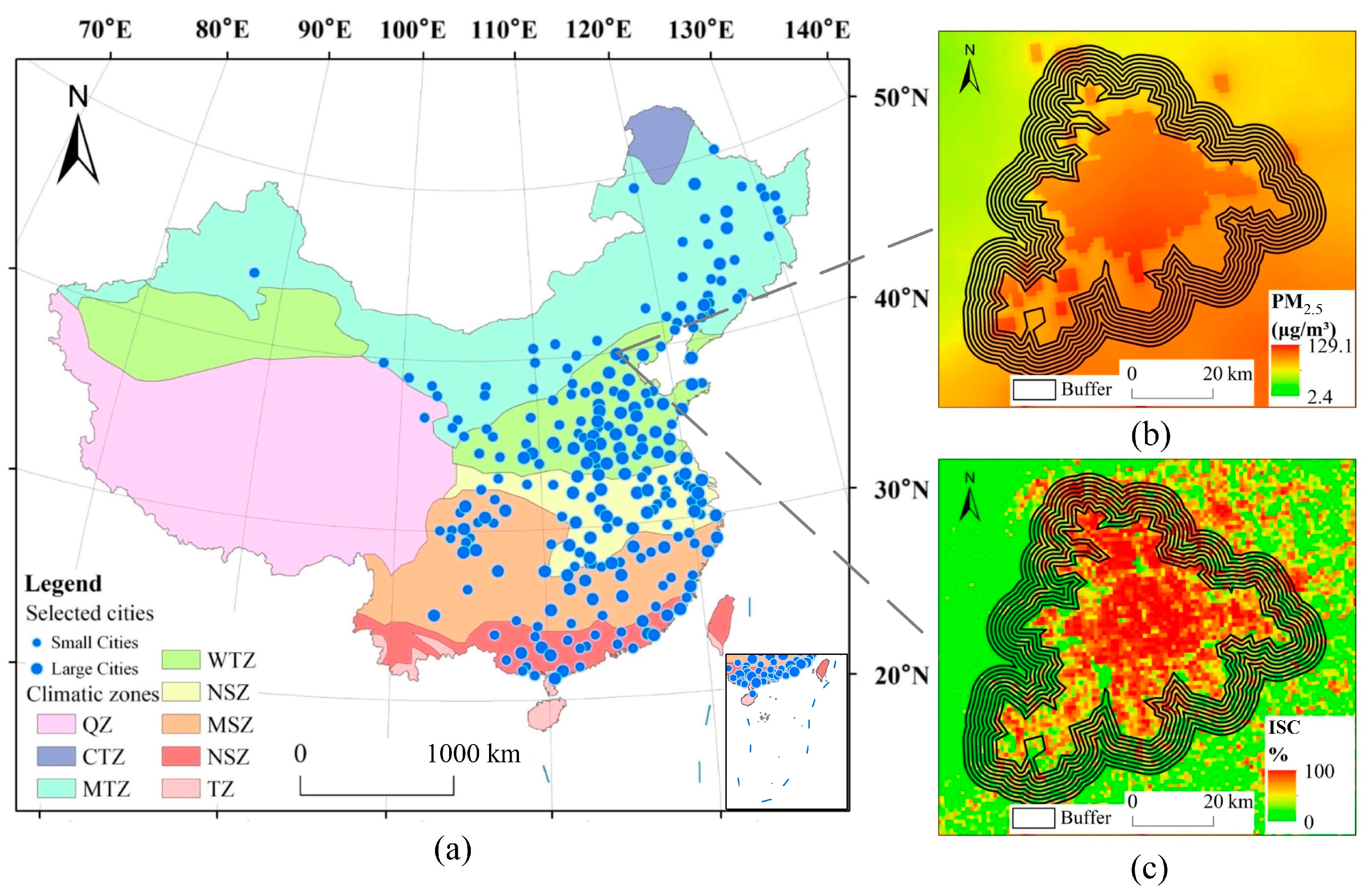
Figure 1 shows the cities selected in the Chinese mainland for the analysis of the spatiotemporal characteristics and driving factors of UPI phenomena. Due to some public statistical data omissions and inconsistent statistical standards, cities with unqualified data were removed. Finally, 240 cities in the Chinese Mainland were chosen for the subsequent experiment and analysis. Additionally, based on the climatic division released by the Institute of Geographic Sciences and Natural Resources Research, Chinese Academy of Sciences, the study area can be divided into five climatic zones, namely, a moderate temperate zone (MTZ, 43 cities), a warm temperate zone (WTZ, 68 cities), a northern subtropical zone (NSZ, 51 cities), a middle subtropical zone (MSZ, 51 cities), and a south subtropical zone (SSZ, 30 cities). Two cities are located in the tropical zone (TZ) and one in the Qinghai–Tibet plateau zone (QZ). Since the number of cities located in these zones is relatively tiny, the analyses in terms of climatic influences did not consider the TZ and QZ. Additionally, following city size divisions in earlier studies [23], the cities selected can be divided into two categories: large (population > 5 million) and small cities (population ≤ 5 million). The numbers of large and small cities included in this study are 147 and 93, respectively.
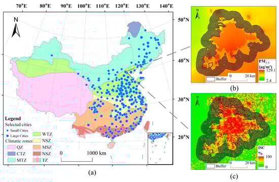
Figure 1.
Overview of the study area: (a) the location of the 240 cities selected; (b) PM2.5 concentrations and the urban–rural gradient in Beijing; (c) impervious surface coverage (ISC—used for urban and rural boundary delineations) in Beijing.
2.2. Data
In order to analyze the spatiotemporal characteristics of UPI effects and their driving factors, the following data were used in this study (Table 2): (1) Gridded PM2.5 concentrations: the data were obtained at a 1 km spatial resolution covering the period 2000–2015 and released by the Atmospheric Composition Analysis Group of Dalhousie University (https://sites.wustl.edu/acag/datasets/surface-pm2-5/ #V4.CH.03, accessed on 24 June 2021). These data were employed for the calculation of PM2.5 concentrations and UPIIs. (2) Impervious surface coverage (ISC): the data were obtained from Kuang et al. (2021) (https://doi.org/10.5281/zenodo.4034161, accessed on 17 September 2020) and were utilized to extract the extent of urban areas [24]. (3) Influencing factors: the driving factors included population density, PM2.5 emission per unit GDP, elevation, precipitation, NDVI, and per capita GDP. Population density and GDP data were collected from the China Urban Statistical Yearbook. Elevation information was obtained from STRM3 (https://srtm.csi.cgiar.org/srtmdata/, accessed on 18 March 2021) and precipitation and NDVI data were acquired from the Institute of Geographic Sciences and Natural Resources Research, CAS (https://www.resdc.cn/data.aspx?DATAID=229, accessed on 27 March 2021). (4) Climatic zone: these data were obtained from the Institute of Geographic Sciences and Natural Resources Research, CAS (https://www.resdc.cn/data.aspx?DATAID=125, accessed on 20 October 2021).
Table 2.
Data used.
2.3. Methods
2.3.1. Overview of the Approach
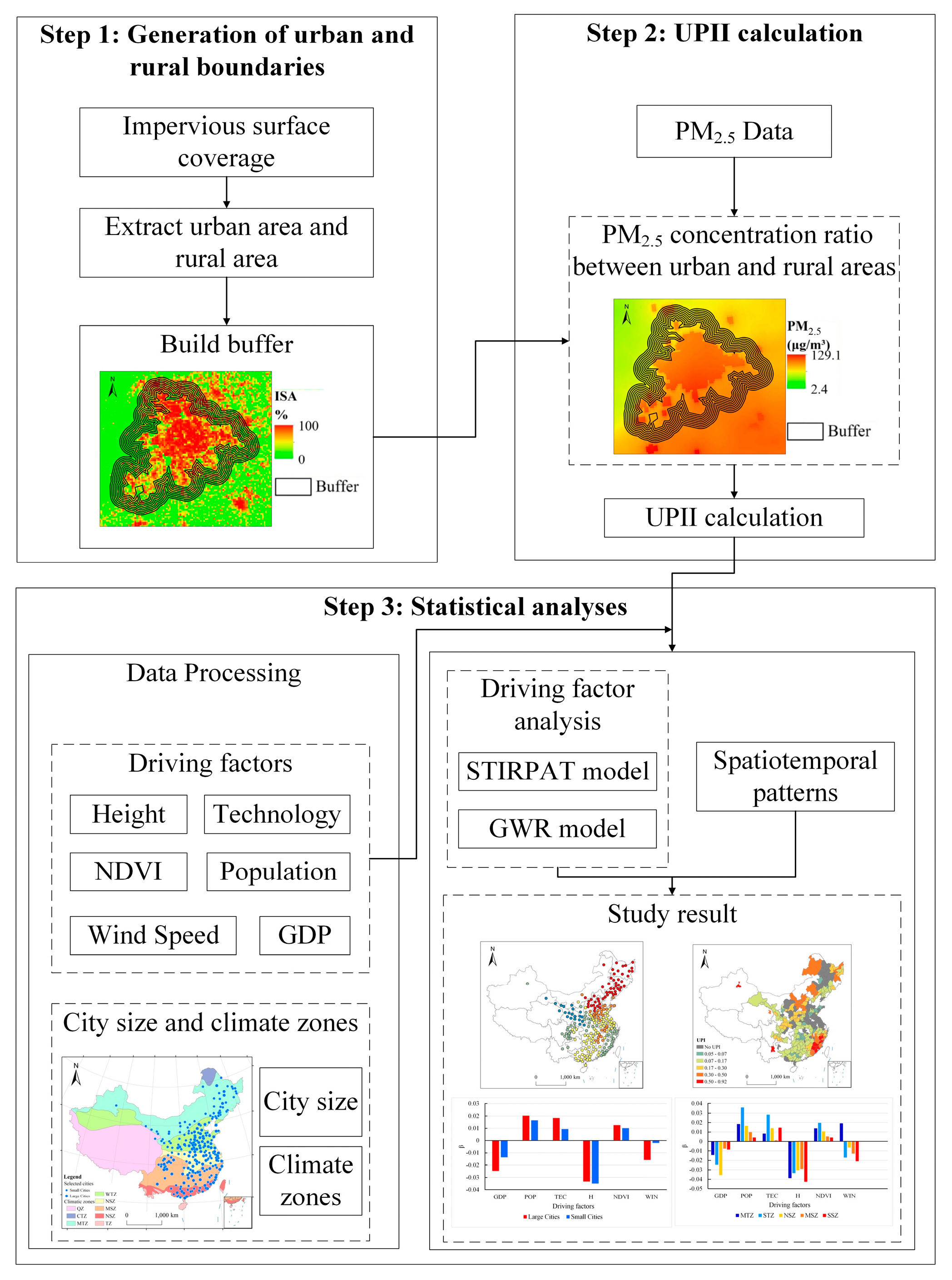
The workflow of the analytical procedure is shown in Figure 2 and includes the following three key steps:

Figure 2.
The workflow of the analytical procedure.
(1) Urban and rural boundary generation: utilizing the ISC data, we extracted urban boundaries and a buffer analysis was further used to determine multiple rural boundaries; (2) UPII calculation: the urban particulate matter island index (UPII) was proposed and employed to investigate UPI phenomena with the assistance of gridded PM2.5 concentration data; (3) investigation of spatiotemporal variations and influencing factors regarding UPI phenomena: we analyzed the spatiotemporal characteristics of UPI phenomena during 2000–2015 and revealed the driving factors of the UPI phenomena using the GWR model.
2.3.2. Generation of Urban and Rural Boundaries
A threshold method based on ISC data was used to determine urban areas. We chose the 25% value of ISC as the threshold value to identify urban areas for the following reason. According to Lu and Weng [25], 25% of ISC can separate medium- and high-intensity residential areas from low-intensity residential areas. Additionally, we employed a buffer analysis with an interval of 1 km to generate eight-layer rural regions (Figure 1b,c).
2.3.3. Definition of UPI
Referring to the method proposed by Cao et al. [6] and the actual needs of driving factor research, the ratio of urban PM2.5 concentrations to background PM2.5 concentrations was used to reflect the urban–rural difference in PM2.5 concentrations and the spatiotemporal characteristics of UPI phenomena. The equation is as follows:
where represents the urban–rural ratio of PM2.5 concentrations; represents urban PM2.5 concentrations; represents background PM2.5 concentrations, which are theoretical PM2.5 concentrations in rural areas and are not disturbed by urban areas under ideal conditions. In actual calculations, the minimum PM2.5 concentration of the three buffer zones farthest from the corresponding urban regions was denoted [5].
In order to characterize urban–rural differences in PM2.5 concentrations more concisely and straightforwardly, a new index, UPII, is defined as:
where represents the intensity of an urban particulate matter island effect. A positive (negative) value for means that the PM2.5 concentration in urban areas is higher (lower) than in rural areas. Note that when the value for a city was >0.05, the city was considered to exhibit a UPI phenomenon [6].
2.3.4. The SIRPAT Model
Ehrlich and Holdren [26] first proposed the impact of population, affluence, and technology (IPAT) model to explore the impact of human activities on environmental issues. Subsequently, Dietz and Rosa improved the IPAT model using a nonlinear stochastic model, i.e., the STIRPAT model [27]. The model can be described as follows:
where represents the PM2.5 concentration difference between urban and rural areas; P, A, and T represent urban–rural differences in population, affluence, and technology impacts, respectively; a is the constant term; b, c, and d represent underdetermined parameters of P, A, and T, respectively; e refers to the random disturbance; and i is the city selected.
Using natural logarithmic transformation, Equation (3) can be described as follows:
where , , and represent urban–rural differences in population, affluence, and technology impacts in the city in Equation (4), respectively. We chose population density, per capita GDP, and PM2.5 emission per unit GDP to represent the population, affluence, and technology levels, respectively. To keep consistent with the stated earlier, , , and were used as the averaged values of areas with minimum PM2.5 concentrations among the three buffer zones farthest from the corresponding urban regions.
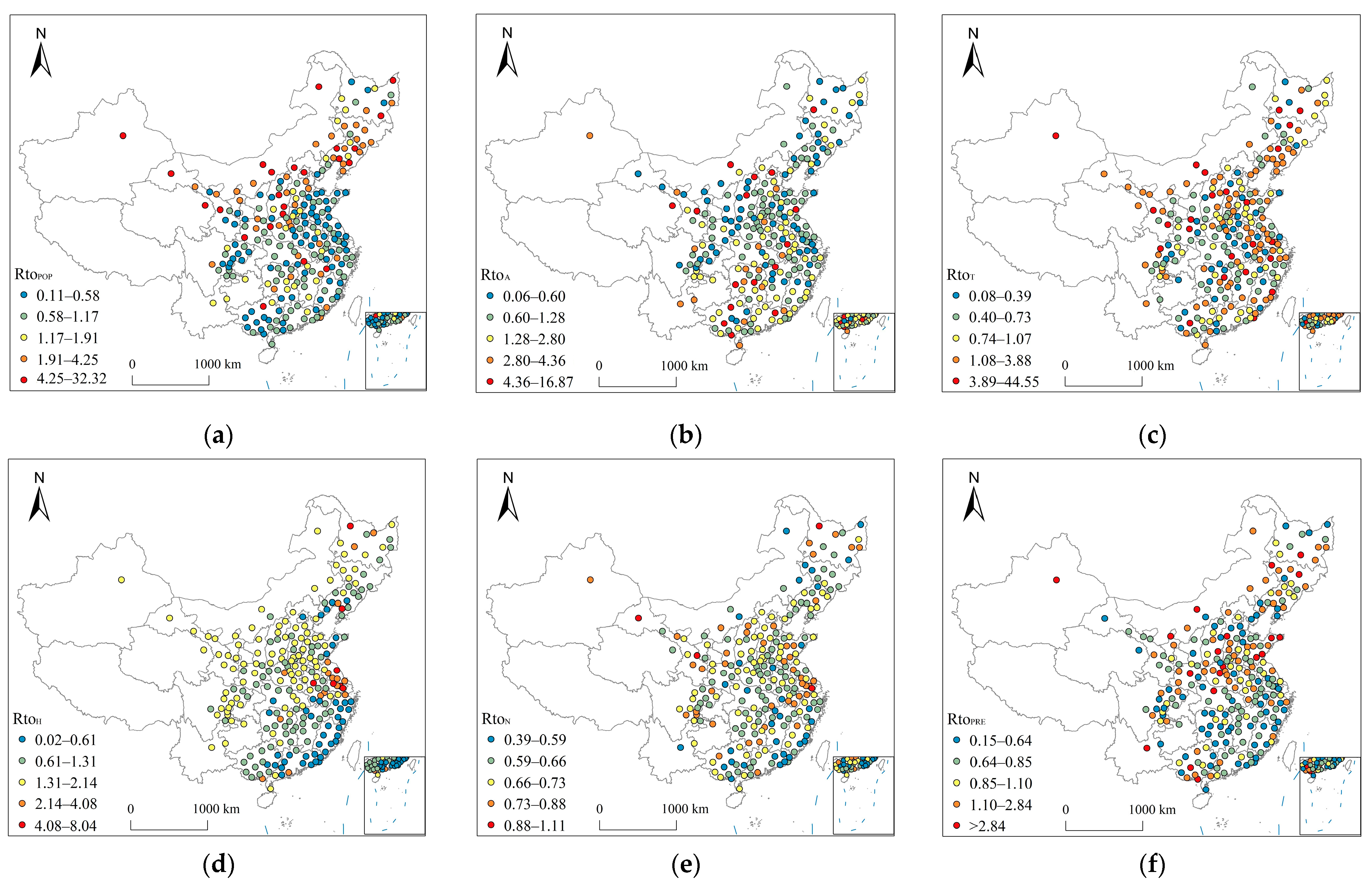
In addition, natural environments also exert a significant influence on the spatial variation in PM2.5 pollution [8]. Accordingly, elevation, precipitation, and NDVI were selected to explain the UPI phenomena. Therefore, more driving factors were introduced to extend Equation (4). Table 3 shows the variables used in the STIRPAT model, and Figure 3 provides the spatial distribution of influencing factors regarding UPI (note that the natural breaks method was utilized to determine the classified ranges of factors). The new model can be described as follows:
where , , and represent urban–rural differences in elevation, precipitation, and NDVI in the city in urban areas, respectively. To simplify Equation (5), , , , , , and can be labeled as , , , , and , respectively, and the final model is:
Table 3.
Variables of the STIRPAT model.
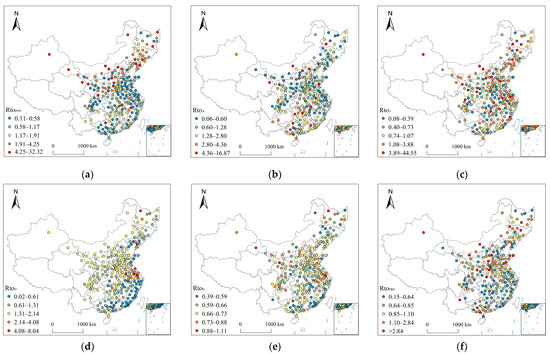
Figure 3.
Spatial distribution of influencing factors regarding UPI: (a) , (b) , (c) , (d) , (e) , and (f) .
Additionally, the mean-subtraction method was utilized to avoid different value ranges among independent variables:
where is the mean-subtracted value of the ith city for each variable, is the average value of each variable in different cities, and is the standard deviation of each variable in different cities.
2.3.5. The GWR Model
The GWR model was employed to determine regression coefficients and can be regarded as a reliable and concise spatial regression method. Compared with the traditional regression model (i.e., ordinary least squares), the GWR model can reflect the impacts of driving factors under varying spatial locations and can be effective when it comes to revealing the local characteristics and regional differences of research objects [28]. It can be calculated as follows [22]:
where is the dependent variable of the city i, i.e., ; is the independent variable and the normalized logarithm of the urban–rural ratio was used for the independent variable in this paper, according to Equation (6); is the random error term; represents the coordinates of the city ; represents the regression coefficients of the city . A positive (or negative) value means that the corresponding factor can increase (or decrease) the value.
The weighted least squares method was used to estimate the regression coefficients of the model [22]:
where is the independent variable matrix, is the dependent variable matrix, and is the spatial weight matrix. Additionally, the Gaussian function was used to calculate the spatial weight matrix [22]:
where is the spatial weight between cities and , is the bandwidth, and is the distance between cities and .
To determine the best bandwidth value, we adopted the corrected Akaike information criterion (AICc) to search for the best value:
where is the maximum likelihood estimate of the variance of the random error term, is the trace of the S-matrix, and is the number of sample cities.
3. Results and Discussion
3.1. Spatiotemporal Pattern of UPIs in China
This section discusses the spatiotemporal variations in UPIs and UPII variations with respect to different climatic settings and city sizes.
3.1.1. Spatial Characteristics of UPIs
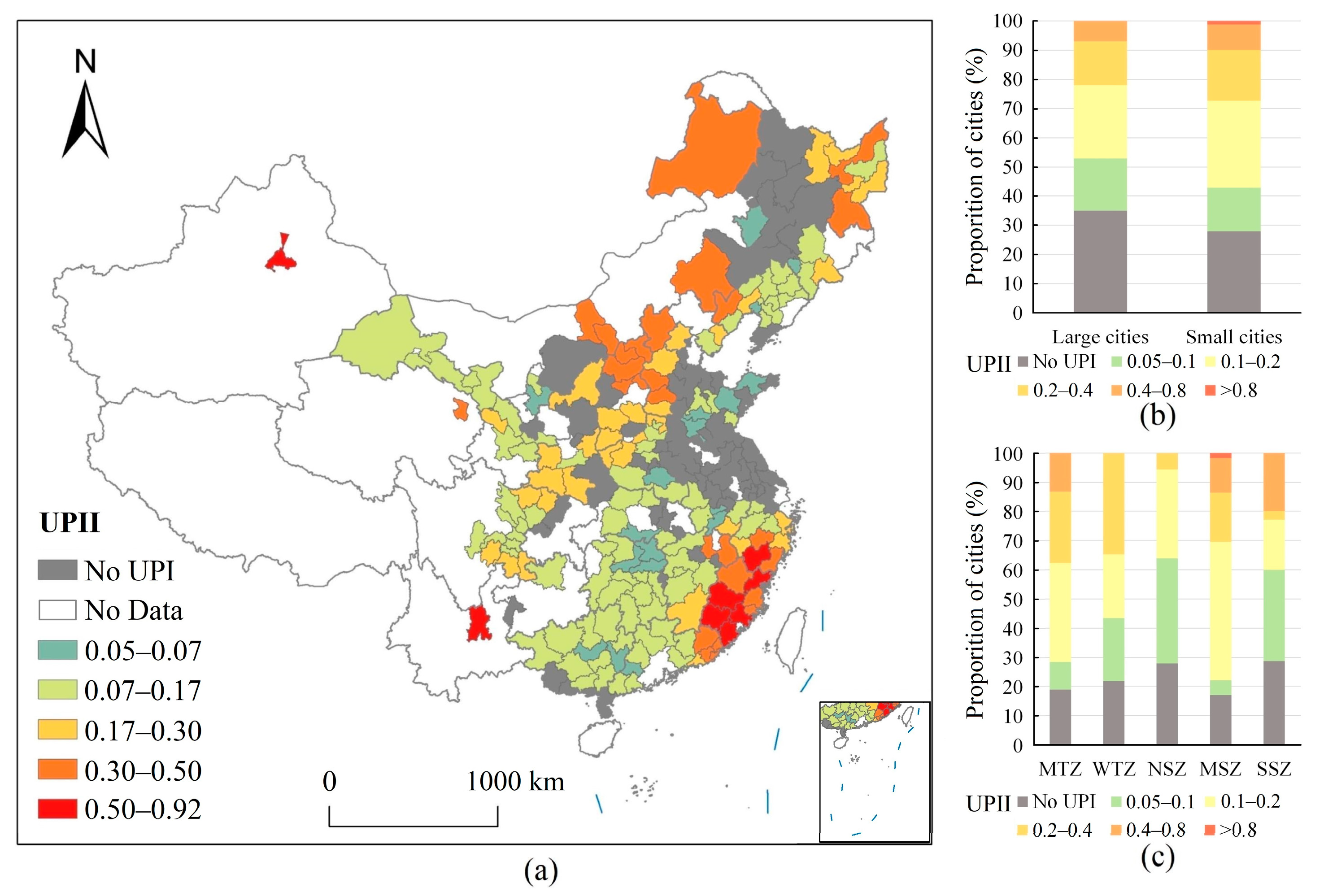
Figure 4 shows the spatial distribution of UPIIs in 240 cities in 2015 and the UPII variations under varying climatic settings and city sizes. The calculation method for the UPII value of each city is based on Equations (1) and (2). As was shown, about 70% of the cities selected yielded obvious UPI phenomena (Figure 4a). Among these, the UPI phenomena were more evident in Zhejiang and Fujian provinces in the southeastern part of China, as well as in Hebei and Shanxi provinces in the northern part of China. UPI phenomena were relatively insignificant in Shandong, Henan, Jiangsu, Anhui, and other provinces in the eastern part of China. In addition, compared with large cities, UPII values in small cities were found to be higher than in large cities (Figure 4b), indicating that city size significantly influences UPI distribution and that the UPI phenomenon is more obvious in small cities. The proportions of cities with UPII values < 0.1 (including cities without UPIs) in small cities (43%) were considerably lower than those in large cities (53%). In addition, only 28% of small cities were without UPIs; in contrast, 35% of large cities were without UPIs. Figure 4c shows UPII values in different climates; it was found that climatic backgrounds had a significant influence on UPI sizes. A rare UPI phenomenon was observed in north subtropical zones. To be specific, cities with UPII values < 0.1 and <0.2 accounted for more than 60% and 94%, respectively. High UPII values were observed in both middle temperate and subtropical zones. In these regions, cities with UPII values >0.4 accounted for >30%.
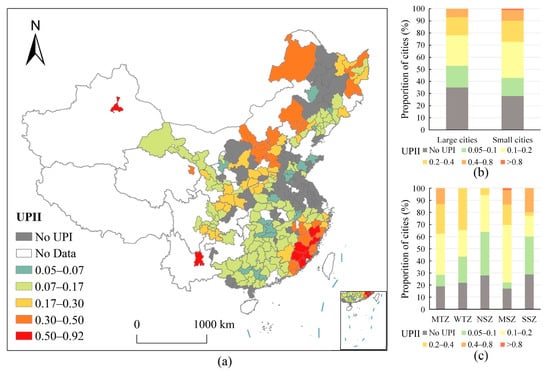
Figure 4.
UPII results for 240 cities selected in 2015: (a) spatial distribution of UPIs; (b) UPIs in large and small cities; (c) UPIs across different climatic backgrounds.
3.1.2. Temporal Variations in UPIs
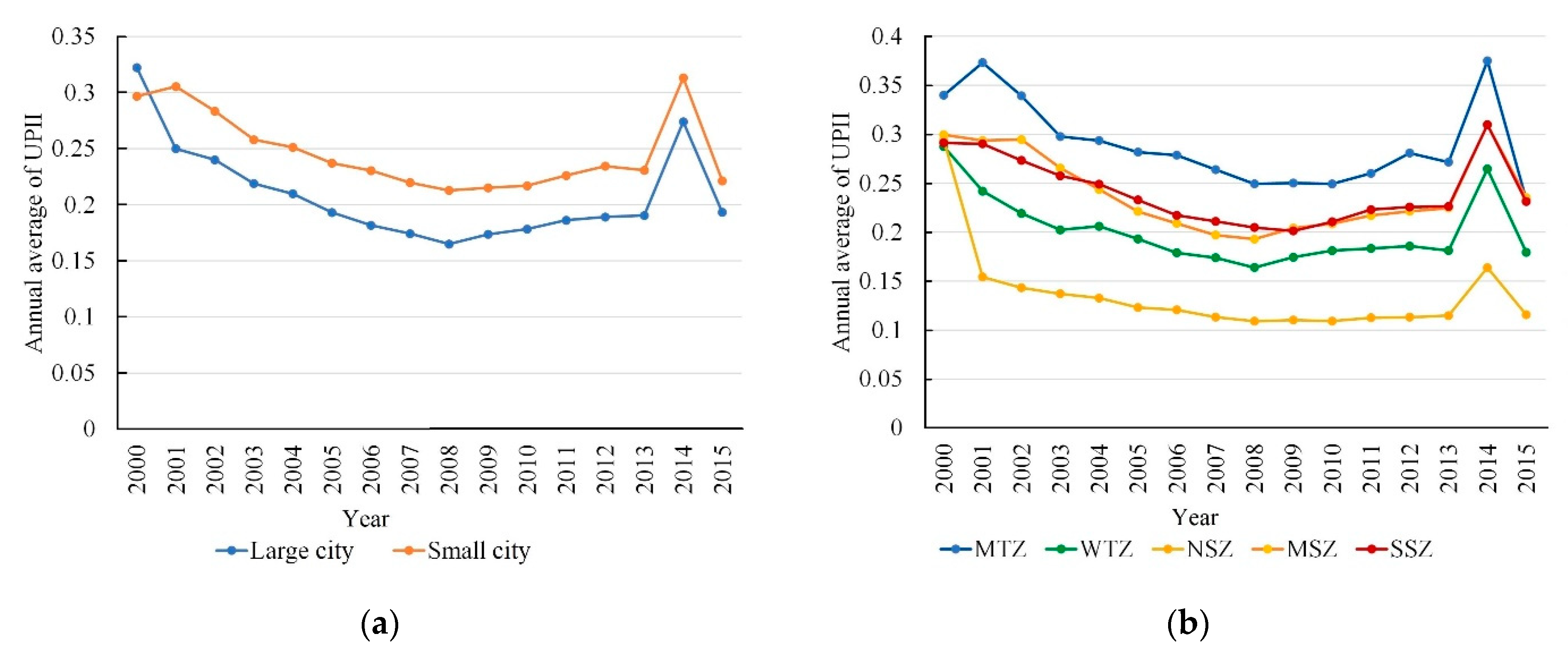
Figure 5 shows temporal variations in the UPIIs of 240 cities of different sizes and with different climate settings from 2000 to 2015. As shown in Figure 5a, generally, decreasing variations in UPIIs were observed in small and large cities over time. The average UPII values in large cities were lower than those in small cities (except for the year 2000). It is noteworthy that slightly increasing variations in UPII values were observed from 2008 to 2014, whereas UPII values significantly decreased from 2000 to 2008. In 2014, the Environmental Protection Law of China was released and in that year many environmental protection measures were implemented that were more severe than previous measures introduced. Many high-pollution industries located in rural areas or near urban areas were forced to move out of rural areas under the influence of laws, resulting in a rise in UPII. Moreover, similar decreasing variations in UPII values in each climate zone were observed (Figure 5b). The ranking of UPII values in different climates from high to low was: MTZ > SSZ (MSZ) > WTZ > NSZ.
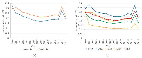
Figure 5.
Temporal variations in UPIIs from 2000 to 2015 for cities of different sizes and with varying climates: (a) UPIs in large and small cities; (b) UPIs across different climatic backgrounds.
Generally speaking, from 2000 to 2015, UPI phenomena existed in most of the selected cities in China, and decreasing variation in UPII values was observed. Previous studies have demonstrated that PM2.5 concentrations in China increased from 2000 to 2015 [29]. Therefore, it can be speculated that increases in PM2.5 concentrations in rural areas led to reductions in UPI phenomena. This suggests that China’s support for rural areas was adequate; however, China is now facing a new problem of PM2.5 pollution shifting from urban to rural areas.
3.2. Driving Factors of UPIs
3.2.1. The Performance of the GWR Model
In order to explore the influence of different driving factors on UPIs, we employed the GWR model to quantify human–environment interactions in relation to shifts and spatial variations in PM2.5 concentrations (details can be found in Equation (8)). The driving factor data were standardized based on Equation (7). The weighted least squares method was used to calculate the regression coefficient, as shown in Equation (9). The Gaussian function was utilized to calculate the spatial weight matrix, as shown in Equation (10). The corrected Akaike information criterion (AICc) was used to determine the best bandwidth value, as shown in Equation (11).
Figure 6 provides the spatial distribution of local R2 values in the GWR model. As shown, the selected model can better detect the relationships between UPII and various factors in most cities. The R2 values of 130 chosen cities were higher than 0.5. The high R2 values were observed in the southeastern and northern parts of China, while the low R2 values were found in the southwestern part of China. This suggests that more influencing factors regarding UPIs should be considered for the cities in the southwestern part of China, e.g., air temperature and secondary industry GDP.
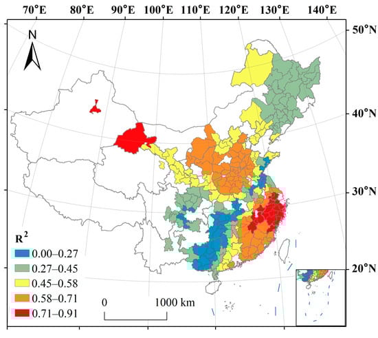
Figure 6.
Spatial distribution of local R2 values in the GWR model.
3.2.2. Results of the GWR Model
Table 4 provides the average β values of the GWR model (note that β stands for the regression coefficient). As shown, all variance inflation factor (VIF) values for the influencing factors were lower than 3, indicating no collinearities between the influencing factors. Generally, RtoP was positively correlated with UPII values, while RtoA, RtoT, RtoH, and RtoPRE were negatively correlated with UPII values. The ranking of the absolute values of regression coefficients from high to low was: RtoH > RtoPRE > RtoP > RtoN > RtoA > RtoT. This suggests that urban–rural differences in elevations exert the most significant influence on RtoUPI. The contributions of natural environments (e.g., precipitation and elevation) to UPI were higher than human activities (e.g., technology and affluence).
Table 4.
Results of the GWR model (the best bandwidth was 60.00). β, regression coefficient; VIF, variance inflation factor.
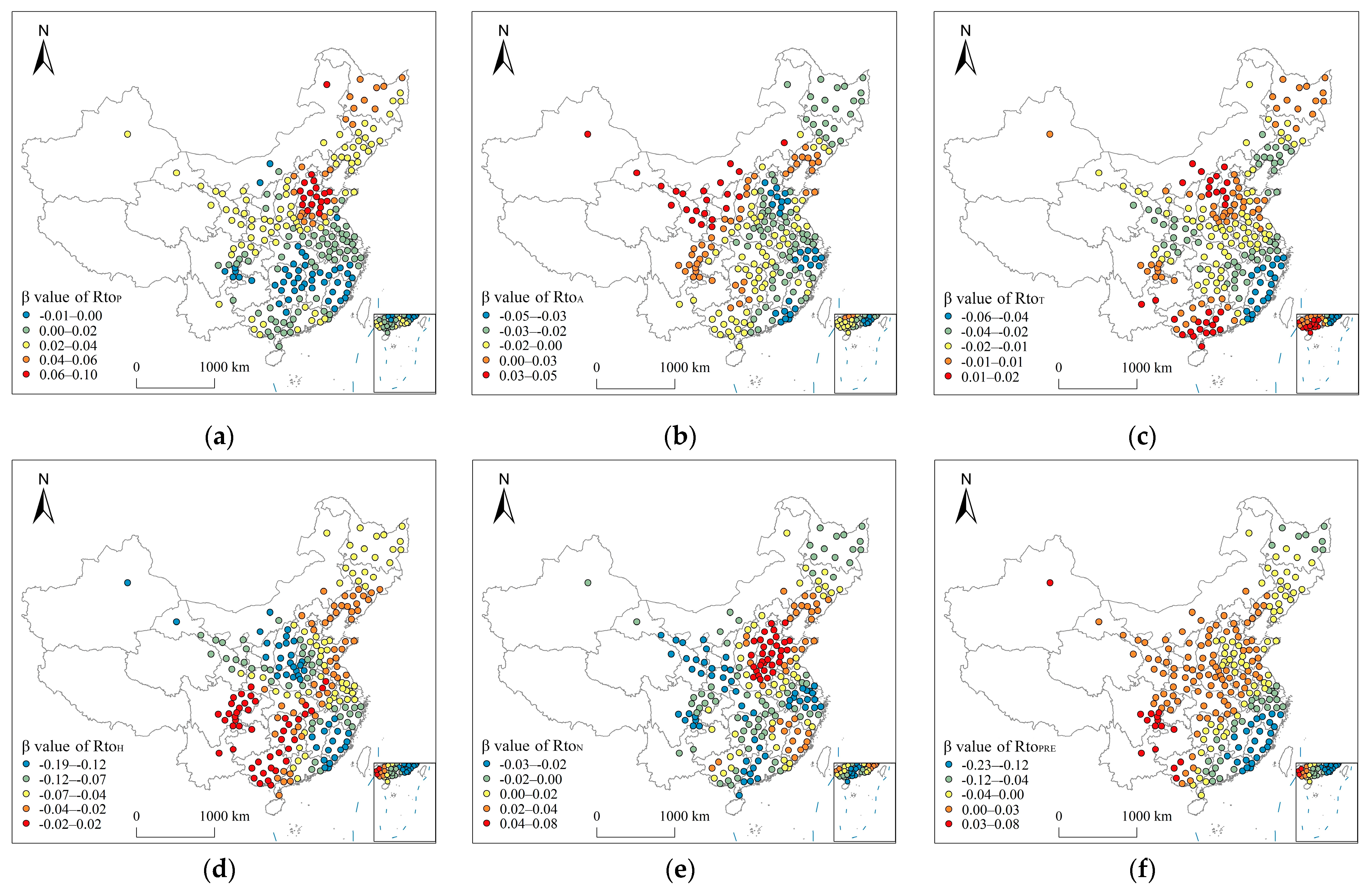
Figure 7 shows the spatial distribution of β values for different influencing factors; we divided β values into five categories based on the natural breaks method. As shown, yielded a positive correlation with RtoUPI in most selected cities (92.92%; Figure 7a), indicating that urban–rural population variations significantly promoted PM2.5 pollution in urban areas and aggravated UPI phenomena. High coefficient values of were found in the northern part of China, especially in the Beijing–Tianjin–Hebei region (BTH) and the northeastern part of Shandong province. This suggests that population shifts from rural to urban areas can significantly increase UPI values. Additionally, low coefficient values (negative β values) of were observed in the southeastern coastal region, indicating that urban–rural differences in human activities in these regions reduced UPI values. One possible reason is that the knowledge population concentrated in urban areas, to some extent, can improve local industrial and technological structures.
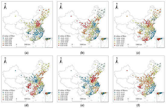
Figure 7.
Spatial distributions of β values: (a) RtoP, (b) RtoA, (c) RtoT, (d) RtoH, (e) RtoN, and (f) RtoPRE.
It was found that was negatively correlated with 77.92% of cities (Figure 7b). This illustrates the fact that the improvement of urban–rural gaps in economies was conducive to inhibiting UPI phenomena for most cities selected. These cities were mainly located in the eastern coastal areas of China. A possible reason is that economic developments were beneficial in terms of optimizing urban production and the lifestyles of residents and thus restraining UPI phenomena. Cities positively correlated with UPI values were mainly located in the western and southeastern coastal areas of China. In these cities, decreasing urban–rural gaps in economies would reduce UPI phenomena, suggesting that economic developments in these regions depend on low-emission industries.
showed negative correlations with UPI values in 75.83% of cities (Figure 7c). Generally, technological progress (which often occurs in urban areas) can improve production efficiencies and reduce PM2.5 emissions in urban areas and thus mitigate UPI phenomena. However, about 20% of cities positively correlated with UPI values were observed in the northern and southern parts of China, i.e., the BTH region.
Figure 7d shows the spatial distribution of β values. As shown, the β values of were negatively correlated with UPI values in 93.33% of cities, indicating that for most cities urban–rural differences in underlying roughness can decrease UPI phenomena. However, it was found that elevation differences between urban and rural areas were positively correlated with UPI values in a few cities in southwestern and northeastern parts of China. A possible reason is that the problematic diffusion of pollution is caused by the complex topography of local mountainous areas.
As for , it was found to be negatively correlated with UPI values in 52.50% of cities (Figure 7e). This indicates that an increase in vegetation is conducive to mitigating PM2.5 pollution. It is noteworthy that cities with positive β values of RtoN were found in the northern part of China, i.e., the Yellow River urban agglomerations (YRUAs). This finding is consistent with the investigations of driving factors of PM2.5 pollution conducted by Mi et al. in the YRUAs [9]. Low vegetation survival rates caused by lack of maintenance may lead to reductions in the positive effects of vegetation and an increase in PM2.5 pollution in these regions [9]. Meanwhile, complicated types and patterns of vegetation distribution may also affect the mitigating influence of vegetation with regard to UPI effects.
It was found that yielded negative correlations with UPI values in 58.75% of cities (Figure 7f), indicating that precipitation can reduce PM2.5 pollution in urban areas and thus conduce to the inhibition of UPI effects. Cities with positive correlations were mainly located in the northeastern and northwestern parts of China. The existing literature shows that a small influence of rainfall on PM2.5 mitigations has been observed in dryer climates, such as Jiangsu province [7] and Beijing [12]; moreover, rainfall, to some extent, can increase PM2.5 concentrations in dry climatic settings.
3.3. Discussion
3.3.1. Dominant Factors Regarding UPIs: Human Activities vs. Physical Environments
The ranking of the influences of various factors on UPI from high to low was: RtoH, RtoPRE, RtoP, RtoN, RtoA, and RtoT. RtoH exerted the most significant influence on the spatiotemporal patterns of UPI. Generally, the effects of natural environments were significantly more potent than those of human activities. It should be noted that, considering the difficulty of regulating natural environments, such as elevation and precipitation, the regulation of human activities is an effective means to control UPI phenomena.
The results of the GWR model show that all factors except the impact of RtoP resulted in pronounced spatial heterogeneity in UPI phenomena. The process of population gathering in cities will increase city sizes, demands for urban construction and transportation, and lead to an increase in PM2.5 pollution in urban areas [11], and thus aggravate UPI phenomena. However, a negative correlation between RtoP and UPI was observed in southeast coastal regions of China, especially in Fujian province. In these regions, the levels of economic development are relatively high [17]. Increased economic development optimizes industrial structures, which can reduce the aggravating effects of RtoP on UPI phenomena. We have shown that during urban expansion, PM2.5 pollution can be controlled through the rational distribution of industrial structures and the optimization of transportation modes and energy structures.
Cities with positive and negative correlations between RtoA and UPI were mainly located in northern and southern parts of China. One possible reason is that high-polluting industries are close to urban areas in the northern part of China. Thus, the widening economic gap between urban and rural will further aggravate UPI phenomena [16]. However, after economic progress and industrial structure regulation in the southern part of China, high-polluting industries in these regions have been reduced [10]. In this situation, the relative growth of urban economies may be caused by a further increase in low-polluting industries and an outflow of high-polluting industries, thus inhibiting UPI phenomena.
RtoT was negatively correlated with UPI in most cities, indicating that the widening technology gap reduces PM2.5 emissions to some extents. Similar to previous studies, technological progress, especially in urban areas, is conducive to improving production efficiency and reducing PM2.5 emissions [19]. Therefore, UPI predominance decreases with the technological gap between urban and rural areas. Nevertheless, technological progress will increase industrial outputs in some central and western cities in China [8], leading to PM2.5 concentrations rising in urban regions. In these cities, the widening gap in technology may result in the relative contraction of industrial outputs, exacerbating UPI phenomena. Therefore, support for and investment in technologies can play a positive role in PM2.5 pollution control. Still, such measures should be taken according to local conditions to avoid the uncontrolled expansion of production, which leads to the worsening of PM2.5 pollution.
For the majority of cities, RtoH has a significant inhibitory effect on UPI phenomena, probably because regions at high elevations can be characterized by diffusions of PM2.5 pollution and increased transportation costs [8]. RtoPRE had a negative correlation with UPI phenomena in most cities selected. Increases in precipitation are conducive to scavenging and reducing local PM2.5 pollution. However, in some western cities in China, especially in Gansu and Sichuan provinces, a positive correlation between RtoPRE and UPI was observed. A possible reason for this is that, in relatively dry environments, precipitation can induce few reductions (and may even cause increases) in PM2.5 pollution. This is basically consistent with the conclusions drawn by Zhou et al. [7] and Zheng et al. [12].
In most cities selected, RtoN yielded negative correlations with UPI, consistent with the existing literature. However, this study found some cities with a positive correlation between RtoN and UPIs and a positive average β value for RtoN. This suggests that NDVI can increase PM2.5 concentrations in some regions, leading to a positive global average value of the regression coefficient. One possible reason is that vegetation is poorly maintained [9] and not well adapted to local environments [30] in these regions and is thus ineffective with regard to purifying air pollution. Meanwhile, NDVI will often increase during some cities’ developments because of environmental protective measures implemented in their construction, but increasing vegetation cannot decrease PM2.5 concentrations [31]. Therefore, studies that focus on vegetation purification are required in the future in order to choose plants that improve local ecological environments and thus avoid the use of those plants that fail to contribute to air pollution control and do not adapt to environmental backgrounds.
3.3.2. The Regulation of Climatic Factors
Climatic backgrounds influenced the compositions and performance of dominant factors regarding UPI phenomena. Table 5 shows the average and standard deviation of β values of influencing factors under varying climatic settings. As shown, climatic backgrounds exerted a significant influence on the performance of driving factors. The urban–rural elevation ratio (RtoH) yielded the most decisive influence in all climatic zones except the south subtropical zone (SSZ). Low mean β values (close to zero) of the urban–rural ratio of NDVI (RtoN) were observed in the moderate temperate zone (MTZ), middle subtropical zone (MSZ), and SSZ. However, the standard deviations of these regions were higher than the mean β values. This suggests that large fluctuations in β values were observed in different cities [8].
Table 5.
The average and standard deviation of regression coefficient values (β) under varying climatic settings.
Additionally, a positive correlation between RtoN and UPI was found in the WTZ [9]. This indicates that, in the WTZ, NDVI can increase PM2.5 pollution. In MTZ, RtoA growth can aggravate UPI phenomena in cities with low levels of urbanization and modernization. A possible reason is that growing economies can exacerbate PM2.5 pollution [10]. In the SSZ, urban–rural ratio precipitation (RtoPRE) yielded the most significant impact on the UPII. In the MTZ, low influences of RtoN, urban–rural affluence ratio (RtoA), and RtoT to UPI were observed; conversely, strong effects of the urban–rural population ratio (RtoP) and RtoH were found. RtoA was observed to be positively correlated with UPI values in the MTZ, while negative correlations between RtoA and UPI values were found in other zones.
3.3.3. The Influence of City Size
Table 6 provides the average and standard deviation of β values concerning influential factors in relation to different city sizes. Generally, the influences of driving factors in large cities were more evident than those in small cities, but the differences were not significant for RtoH, RtoT, and RtoP. As expected, precipitation significantly decreased PM2.5 concentrations and the influence in big cities was more potent than in small cities. This demonstrates that city size can regulate the effect of precipitation on PM2.5 concentrations. In large cities with high urbanization rates [11] and dense populations [17], population density significantly increased PM2.5 concentration, but a difference between large and small cities was not apparent. RtoA was negatively correlated with UPII in large and small cities; however, the link was weak in small cities, i.e., the mean β value was close to zero. This suggests that RtoA growth in big cities yielded a more obvious inhibiting effect on UPI than in small cities. Cities with high economic development were amenable to industrial upgrading and the relocation of heavily polluting industries, which might generate a negative correlation between RtoA and UPIs [10]. As to NDVI, a significantly negative correlation between RtoN and UPII in big cities was observed. However, a slightly positive correlation between RtoN and UPII was found in small cities. This finding suggests that, in big cities, vegetation exerts considerable mitigation of PM2.5 concentrations.
Table 6.
The average and standard deviation of regression coefficient values (β) with different city sizes.
3.3.4. Limitations and Future Research Directions
Several limitations are noted. Firstly, we investigated human–environment interactions in PM2.5 concentrations and considered urban–rural shifts in PM2.5 concentrations. This inevitably led to statistical data being missing for some cities and to inconsistent data. Thus, only 240 cities in China were chosen for this study. Studies that perform spatializations of socioeconomic data (i.e., technology, population, and GDP) are required in the future. Secondly, the GWR analysis results have shown that the R2 values in some cities were less than 0.45. More driving factors should be considered to explore UPI dynamics, e.g., three-dimensional urban morphological parameters, air temperatures, secondary industry GDP, and wind speed.
4. Conclusions
In this study, choosing 240 cities in China, we investigated the spatiotemporal characteristics of UPIs in varying climatic settings and urban settings. Additionally, human–environment interactions in UPI dynamics were explored using the GWR model. At last, we analyzed how climatic zones and city sizes regulate the compositions of dominant factors. The main conclusions that can be drawn are as follows:
(1) The majority of cities selected exhibited UPI phenomena. Premature death will be increased due to long-term exposure to higher concentrations of PM2.5. Due to urbanization, the urban population has increased significantly. As a result, UPI phenomena mean an increase in the number of people exposed to high levels of PM2.5 pollution, with negative impacts on the health of urban residents. It was found that UPI phenomena in small cities are more severe than those in big cities. The UPI phenomena in MTZ and SSZ were more potent than in other climatic settings. UPI phenomena have shown decreasing trends over time, indicating that China’s support for rural areas was adequate; however, China is now facing a new problem of PM2.5 pollution shifting from urban to rural areas.
(2) The ranking of the absolute values of regression coefficients (based on the GWR model) from high to low was: RtoH > RtoPRE > RtoP > RtoN > RtoA > RtoT. This suggests that urban–rural differences in elevations exert the most significant influence on RtoUPI. The contributions of natural environments (e.g., precipitation and elevation) to UPIs were higher than human activities (e.g., technology and affluence).
(3) It was found that urban–rural population variations significantly promoted PM2.5 pollution in urban areas and aggravated UPI phenomena. The improvement of urban–rural gaps in economies was conducive to inhibiting UPI phenomena. Generally, technological progress (which often occurs in urban areas) can improve production efficiencies and reduce PM2.5 emissions in urban areas, thus mitigating UPI phenomena. Similarly, urban–rural differences in underlying roughness can decrease UPI phenomena. As expected, an increase in vegetation is conducive to mitigating PM2.5 pollution. Precipitation can reduce PM2.5 pollution in urban areas and thus be conducive to inhibiting UPI effects.
(4) Climatic backgrounds influenced the compositions and performance of dominant factors regarding UPI phenomena. Generally, the influences of driving factors in large cities were more evident than those in small cities, but the differences were not significant for RtoH, RtoT, and RtoP.
The contributions of the study can be summarized as follows. First, it shows how human–environmental factors interact to influence UPI spatiotemporal variations with respect to various climatic settings and city sizes, which is something that has rarely been reported in previous studies. Second, it provides a clear picture of how climatic backgrounds and city sizes regulate the compositions of dominant factors to impact UPI variations. This is of importance since it is valuable for PM2.5 pollution mitigation in cities experiencing global climate change and rapid urbanization and thus can help sustainable urban developments.
Author Contributions
Conceptualization, Z.P. and S.C.; methodology, Z.P. and M.Y.; validation, S.C., M.D., and W.Z.; formal analysis, Z.P.; investigation, Z.P. and L.L.; resources, M.D and S.C.; data curation, Z.P., M.Y., and Y.C.; writing—original draft preparation, Z.P.; writing—review and editing, S.C., M.D., and W.Z.; visualization, Z.P., Y.C., and Y.M.; supervision, S.C. All authors have read and agreed to the published version of the manuscript.
Funding
This research was supported by the National Natural Science Foundation (NSFC) (Key Project #41930650).
Institutional Review Board Statement
Not applicable.
Informed Consent Statement
Not applicable.
Data Availability Statement
The UPI data are available on request to the corresponding author.
Conflicts of Interest
The authors declare no conflict of interest. The funders had no role in the design of the study; in the collection, analyses, or interpretation of data; in the writing of the manuscript, or in the decision to publish the results.
Nomenclature
| Nomenclature | Definition |
| AIC | Akaike Information Criterion |
| AICc | Corrected Akaike Information Criterion |
| ARDL | Auto-regressive distributed lag |
| BTH | Beijing–Tianjin–Hebei region |
| CTZ | Cold temperate zone |
| GDIM | Generalized Divisia index method |
| GDP | Gross domestic product |
| GWR | Geographically Weighted Regression |
| IPAT | Impact of population, affluence, and technology |
| ISC | Impervious surface coverage |
| LUR | Land Use Regression |
| MGWR | Multi-scale Geographically Weighted Regression |
| MSZ | Middle subtropical zone |
| MTZ | Moderate temperate zone |
| NDVI | Normalized difference vegetation index |
| NSZ | Northern subtropical zone |
| OLS | Ordinary Least Squares |
| QR | Quantile regression |
| QZ | Qinghai–Tibet plateau zone |
| Rto | Urban–rural ratio |
| RtoA | Urban–rural ratio of GDP |
| RtoH | Urban–rural ratio of elevation |
| RtoN | Urban–rural ratio of NDVI |
| RtoP | Urban–rural ratio of population |
| RtoPRE | Urban–rural ratio of annual mean precipitation |
| RtoT | Urban–rural ratio of PM2.5 pollution emitted per unit GDP |
| SSZ | South subtropical zone |
| STIRPAT | Stochastic impacts by regression on population, affluence, and technology |
| TZ | Tropical zone |
| UPI | Urban particulate matter island |
| UPII | Urban particulate matter island intensity |
| VIF | Variance inflation factor |
| WTZ | Warm temperate zone |
| YRUA | Yellow River urban agglomerations |
| β | Regression coefficient by the GWR model |
References
- Pope, C.A.; Brook, R.D.; Burnett, R.T.; Dockery, D.W. How Is Cardiovascular Disease Mortality Risk Affected by Duration and Intensity of Fine Particulate Matter Exposure? An Integration of the Epidemiologic Evidence. Air Qual. Atmos. Health 2011, 4, 5–14. [Google Scholar] [CrossRef]
- Wang, F.; Ahat, X.; Liang, Q.; Ma, Y.; Sun, M.; Lin, L.; Li, T.; Duan, J.; Sun, Z. The Relationship between Exposure to PM2.5 and Atrial Fibrillation in Older Adults: A Systematic Review and Meta-Analysis. Sci. Total Environ. 2021, 784, 147106. [Google Scholar] [CrossRef]
- Yu, P.; Xu, R.; Coelho, M.; Paulo, H.; Li, S.; Zhao, Q.; Mahal, A.; Sim, M.; Abramson, M.; Guo, Y. The Impacts of Long-Term Exposure to PM 2.5 on Cancer Hospitalizations in Brazil. Environ. Int. 2021, 154, 106671. [Google Scholar] [CrossRef]
- Li, Y.; Liao, Q.; Zhao, X.; Tao, Y.; Bai, Y.; Peng, L. Premature Mortality Attributable to PM2.5 Pollution in China during 2008–2016: Underlying Causes and Responses to Emission Reductions. Chemosphere 2021, 263, 127925. [Google Scholar] [CrossRef]
- Huang, X.; Cai, Y.; Li, J. Evidence of the Mitigated Urban Particulate Matter Island (UPI) Effect in China during 2000–2015. Sci. Total Environ. 2019, 660, 1327–1337. [Google Scholar] [CrossRef]
- Cao, Y.; Fang, X.; Wang, J.; Li, G.; Li, Y. Measuring the Urban Particulate Matter Island Effect with Rapid Urban Expansion. Int. J. Environ. Res. Public Health 2020, 17, 5535. [Google Scholar] [CrossRef]
- Zhou, B.; Liu, D.; Yan, W. A Simple New Method for Calculating Precipitation Scavenging Effect on Particulate Matter: Based on Five-Year Data in Eastern China. Atmosphere 2021, 12, 759. [Google Scholar] [CrossRef]
- Wang, S.; Liu, X.; Yang, X.; Zou, B.; Wang, J. Spatial Variations of PM2.5 in Chinese Cities for the Joint Impacts of Human Activities and Natural Conditions: A Global and Local Regression Perspective. J. Clean. Prod. 2018, 203, 143–152. [Google Scholar] [CrossRef]
- Mi, Y.; Sun, K.; Li, L.; Lei, Y.; Wu, S.; Tang, W.; Wang, Y.; Yang, J. Spatiotemporal Pattern Analysis of PM2.5 and the Driving Factors in the Middle Yellow River Urban Agglomerations. J. Clean. Prod. 2021, 299, 126904. [Google Scholar] [CrossRef]
- Zhao, H.; Guo, S.; Zhao, H. Characterizing the Influences of Economic Development, Energy Consumption, Urbanization, Industrialization, and Vehicles Amount on PM2.5 Concentrations of China. Sustainability 2018, 10, 2574. [Google Scholar] [CrossRef]
- Wang, S.; Xu, L.; Ge, S.; Jiao, J.; Pan, B.; Shu, Y. Driving Force Heterogeneity of Urban PM2.5 Pollution: Evidence from the Yangtze River Delta, China. Ecol. Indic. 2020, 113, 106210. [Google Scholar] [CrossRef]
- Zheng, Z.; Xu, G.; Li, Q.; Chen, C.; Li, J. Effect of Precipitation on Reducing Atmospheric Pollutant over Beijing. Atmos. Pollut. Res. 2019, 10, 1443–1453. [Google Scholar] [CrossRef]
- Li, X.; Zhang, C.; Li, W.; Liu, K. Evaluating the Use of DMSP/OLS Nighttime Light Imagery in Predicting PM2.5 Concentrations in the Northeastern United States. Remote Sens. 2017, 9, 620. [Google Scholar] [CrossRef] [Green Version]
- Wei, F.; Li, S.; Liang, Z.; Huang, A.; Wang, Z.; Shen, J.; Sun, F.; Wang, Y.; Wang, H.; Li, S. Analysis of Spatial Heterogeneity and the Scale of the Impact of Changes in PM2.5 Concentrations in Major Chinese Cities between 2005 and 2015. Energies 2021, 14, 3232. [Google Scholar] [CrossRef]
- Jin, Q.; Fang, X.; Wen, B.; Shan, A. Spatio-Temporal Variations of PM2.5 Emission in China from 2005 to 2014. Chemosphere 2017, 183, 429–436. [Google Scholar] [CrossRef]
- Wu, D.; Zhang, F.; Ge, X.; Yang, M.; Xia, J.; Liu, G.; Li, F. Chemical and Light Extinction Characteristics of Atmospheric Aerosols in Suburban Nanjing, China. Atmosphere 2017, 8, 149. [Google Scholar] [CrossRef] [Green Version]
- Han, L.; Zhou, W.; Li, W.; Qian, Y. Urbanization Strategy and Environmental Changes: An Insight with Relationship between Population Change and Fine Particulate Pollution. Sci. Total Environ. 2018, 642, 789–799. [Google Scholar] [CrossRef]
- Yu, Y.; Zhou, X.; Zhu, W.; Shi, Q. Socioeconomic Driving Factors of PM2.5 Emission in Jing-Jin-Ji Region, China: A Generalized Divisia Index Approach. Environ. Sci. Pollut. Res. 2021, 28, 15995–16013. [Google Scholar] [CrossRef]
- Cheng, Z.; Li, L.; Liu, J. Identifying the Spatial Effects and Driving Factors of Urban PM2.5 Pollution in China. Ecol. Indic. 2017, 82, 61–75. [Google Scholar] [CrossRef]
- Larkin, A.; van Donkelaar, A.; Geddes, J.A.; Martin, R.V.; Hystad, P. Relationships between Changes in Urban Characteristics and Air Quality in East Asia from 2000 to 2010. Environ. Sci. Technol. 2016, 50, 9142–9149. [Google Scholar] [CrossRef] [Green Version]
- Rowe, D.B. Green Roofs as a Means of Pollution Abatement. Environ. Pollut. 2011, 159, 2100–2110. [Google Scholar] [CrossRef] [PubMed] [Green Version]
- Brunsdon, C.; Fotheringham, A.S.; Charlton, M.E. Geographically Weighted Regression: A Method for Exploring Spatial Nonstationarity. Geogr. Anal. 1996, 28, 281–298. [Google Scholar] [CrossRef]
- Bressi, M.; Sciare, J.; Ghersi, V.; Bonnaire, N.; Nicolas, J.B.; Petit, J.-E.; Moukhtar, S.; Rosso, A.; Mihalopoulos, N.; Féron, A. A One-Year Comprehensive Chemical Characterisation of Fine Aerosol (PM 2.5) at Urban, Suburban and Rural Background Sites in the Region of Paris (France). Atmos. Chem. Phys. 2013, 13, 7825–7844. [Google Scholar] [CrossRef] [Green Version]
- Kuang, W.; Zhang, S.; Li, X.; Lu, D. A 30 m Resolution Dataset of China’s Urban Impervious Surface Area and Green Space, 2000–2018. Earth Syst. Sci. Data 2021, 13, 63–82. [Google Scholar] [CrossRef]
- Lu, D.; Weng, Q. Use of Impervious Surface in Urban Land-Use Classification. Remote Sens. Environ. 2006, 102, 146–160. [Google Scholar] [CrossRef]
- Ehrlich, P.R.; Holdren, J.P. Impact of Population Growth. Science 1971, 171, 1212–1217. [Google Scholar] [CrossRef]
- Dietz, T.; Rosa, E.A. Rethinking the Environmental Impacts of Population, Affluence and Technology. Hum. Ecol. Rev. 1994, 1, 277–300. [Google Scholar]
- Fotheringham, A.S.; Charlton, M.E.; Brunsdon, C. Geographically Weighted Regression: A Natural Evolution of the Expansion Method for Spatial Data Analysis. Environ. Plan. A 1998, 30, 1905–1927. [Google Scholar] [CrossRef]
- Shisong, C.; Wenji, Z.; Hongliang, G.; Deyong, H.; You, M.; Wenhui, Z.; Shanshan, L. Comparison of Remotely Sensed PM2.5 Concentrations between Developed and Developing Countries: Results from the US, Europe, China, and India. J. Clean. Prod. 2018, 182, 672–681. [Google Scholar] [CrossRef]
- Hajiloo, F.; Hamzeh, S.; Gheysari, M. Impact Assessment of Meteorological and Environmental Parameters on PM 2.5 Concentrations Using Remote Sensing Data and GWR Analysis (Case Study of Tehran). Environ. Sci. Pollut. Res. 2019, 26, 24331–24345. [Google Scholar] [CrossRef]
- Huang, B.; Li, Z.; Dong, C.; Zhu, Z.; Zeng, H. The Effects of Urbanization on Vegetation Conditions in Coastal Zone of China. Prog. Phys. Geogr. Earth Environ. 2021, 45, 564–579. [Google Scholar] [CrossRef]

Publisher’s Note: MDPI stays neutral with regard to jurisdictional claims in published maps and institutional affiliations. |
© 2022 by the authors. Licensee MDPI, Basel, Switzerland. This article is an open access article distributed under the terms and conditions of the Creative Commons Attribution (CC BY) license (https://creativecommons.org/licenses/by/4.0/).