Article

Mapping the Spatial Heterogeneity of Anthropogenic Soil Nitrogen Net Replenishment Based on Soil Loss: A Coastal Case in the Yellow River Delta, China

1
State Key Laboratory of Resources and Environmental Information System, Institute of Geographic Sciences and Natural Resources Research, Chinese Academy of Sciences, Beijing 100101, China
2
University of Chinese Academy of Sciences, Beijing 100049, China
3
Jiangsu Center for Collaborative Innovation in Geographical Information Resource Development and Application, Nanjing 210023, China
*
Authors to whom correspondence should be addressed.
These authors contributed equally to this work.
Sustainability 2022, 14(10), 6078; https://doi.org/10.3390/su14106078
Submission received: 23 March 2022 / Revised: 4 May 2022 / Accepted: 12 May 2022 / Published: 17 May 2022

Abstract

:
To explore the spatial heterogeneity of nitrogen supply from human activities to soil in coastal areas, we established a soil nitrogen net replenishment index (A-SNNRI). We applied the Revised Universal Soil Loss Equation (RUSLE) model for soil loss risk calculation and geostatistical analysis for process simulation. A case study in the Yellow River Delta (YRD) showed that the A-SNNRI worked well. During the summer crop-growing season, population and land use presented significant influences on the soil total nitrogen (STN) status. Urban villages and arable land both had the largest summary STN and variety. There was a negative correlation between STN change and soil loss. The east coast held both the largest A-SNNRIs and soil loss risks. There were significant positive correlations between A-SNNRIs and population and GDP. Therefore, to control and reduce soil-source nitrogen exports in the YRD, we need to reduce nitrogen emissions from urban villages, agriculture, industry, and aquaculture and determine the main risk locations along the east coast and in the main city.

1. Introduction

In recent years, China has faced several environmental problems due to the high intensity of land development and utilization in coastal areas [1,2]. However, the future of coastal water ecological environments is not optimistic, as these areas suffer from severe nitrogen pollution. With the development of the social economy, coastal human-made sources have become the main causes of marine pollution [3]. Among the terrestrial pollution source processes, nitrogen pollutants entering water bodies in the form of soil erosion account for a larger portion, forming serious nonpoint source pollution [4,5]. Simultaneously, soil nitrogen replenishment from crop planting has become the main source of soil nitrogen losses in agricultural areas [6,7,8]. Therefore, for pollution control, it is important to sort out the influence of human activities on soil nitrogen replenishment, yet the amount of replenishment is difficult to quantify spatially because it contains a comprehensive process of multiple increments and decrements [9,10]. However, the main processes of soil nitrogen loss are vegetation consumption and soil loss [11,12,13], and the final status of the comprehensive process of soil nitrogen gains and losses can be reflected in the soil nitrogen storage [14,15]. At present, relevant studies have focused separately on the spatiotemporal variation in soil nitrogen [16,17] and the loss of soil sediment [18,19,20]. Few researchers have focused on soil nitrogen replenishment from human activity and soil loss perspectives.
The soil loss process is related to several ecological environmental factors, including the soil texture conditions, rainfall intensity, topography, and land cover [21,22]. Of the existing soil loss research methods, the Revised Universal Soil Loss Equation (RUSLE) is currently the most scientific and accurate method for the calculation of soil loss and has been widely used in recent decades [23,24,25]. However, the RUSLE is usually applied to analyse the quantity of sediment that enters the water body due to rainfall scouring the soil surface [26,27] and never involves loss analyses of concrete soil pollutants.
Human activities and the natural geographic environment both exhibit heterogeneity, which leads to spatial differences in the potential for soil nitrogen replenishment and pollutant outputs. Therefore, these environmental problems also need to be solved from the perspective of spatial heterogeneity [28,29,30]. With the rapid development of geographic science and computer technology, it is possible to present and visualize the spatial heterogeneity of geographic phenomena. In recent years, the advantages of geographic information systems (GISs) in spatial data analysis and spatiotemporal problem positioning have gradually become prominent. Using GIS tools to understand spatial heterogeneity not only works well in obtaining the location of key issues but also plays the initial roles in proposing target solutions [31,32,33,34,35].
The Yellow River Delta (YRD), located close to Laizhou Bay, is a typical coastal plain with an intense number of human activities. In recent years, Laizhou Bay has experienced serious land-based pollution problems [36,37,38,39,40]. The discharge of industrial and agricultural nitrogen pollutants from the YRD poses greater threats to the adjacent Laizhou Bay [41,42,43]. From the land source reduction perspective, it is highly important to accurately and spatially understand the nitrogen emission risks imposed by human activities in the YRD for the prevention and control of coastal water pollution. Therefore, this research selected the YRD as a typical coastal zone region and established a method for calculating the risk of soil nitrogen replenishment under the influence of human activities, and this method is called the anthropogenic soil nitrogen net replenishment index (A-SNNRI). In the A-SNNRI, we mainly considered the soil nitrogen status and loss risks during soil erosion and realized a two-dimensional layered analysis by applying geospatial methods. We calculated the soil nitrogen loss risks based on the RUSLE model. For the analysis of human impact, we applied land use, population, and gross domestic product (GDP) for relevant geostatistics and correlation analysis. Our objective was to obtain the distribution characteristics of anthropogenic nitrogen replenishment to the soil environment in the study area and determine the main influencing factors. Then, we propose temporal and spatially targeted strategies for the control and reduction of into-sea nitrogen nonpoint source pollution emissions.

2. Materials and Methods

2.1. Study Region

The study area is the YRD (118°13′–119°17′ E, 37°16′–37°50′ N), China. It is located between the Yellow River and the Zhimai River, and Laizhou Bay is in the east (see Figure 1). The total area is 2902 km2. It is a typical estuary delta in the coastal zone with serious land–sea interactions, half of which was formed by extremely rapid sedimentation of the Yellow River in the last 200 years [44], promoting one of the youngest lands in the world [45,46]. The terrain is flat with an average elevation of 3 m. The YRD belongs to a temperate continental monsoon climate. Rainfall is mainly concentrated in the summer season, and the average annual precipitation is approximately 550 mm [47]. In terms of administrative divisions, our research area was located in Shandong Province, China, consisting of Dongying District and Kenli District. The Second Land Use Survey of China showed that arable land and urban villages make up 24% and 10%, respectively. Industry and agriculture have relatively high economic shares in this region (http://tjj.shandong.gov.cn/tjnj/ (accessed on 30 December 2020)). There is a twice-a-year crop ripening system. The main planting crops are corn, rice, soybeans, and cotton in summer and wheat in winter, which often consume larger amounts of fertilizers and pesticides in summer. In addition, there was 15% saline-alkali land, and the soil salinity was relatively high. There was an average pH value of 8.31 and salt content of 5.84 g/kg (soil sampling data of the 0–20 cm topsoil in 2019). Moreover, the sea distribution was a negative factor for the soil fertility and vegetation cover. There are relatively high soil erosion risks [48,49,50].

2.2. Data Collection

2.2.1. Soil Sampling and Laboratory Analysis

Agricultural nitrogen supplements are the main source of soil nitrogen in the YRD [51]. To consider the influence of agricultural planting on soil nitrogen, we carried out two periods of soil sampling, in June and October 2020, before and after the summer crop-growing season, respectively. A total of 125 soil samples were collected in June, and 127 samples were collected in October, with a 3 km × 3 km sampling density (see Figure 1a). The soil sampling depth was 0–20 cm. We implemented a homogeneous-mix process for each soil sample. Then, the soil samples were sealed and frozen after being collected and subjected to a laboratory analysis of composition. The measurement indicators included soil organic matter (SOM) (No. GB 7857-87 of Chinese standard) and soil total nitrogen (STN) (No. HJ 717-2014 of Chinese standard).

2.2.2. Auxiliary Spatial Data

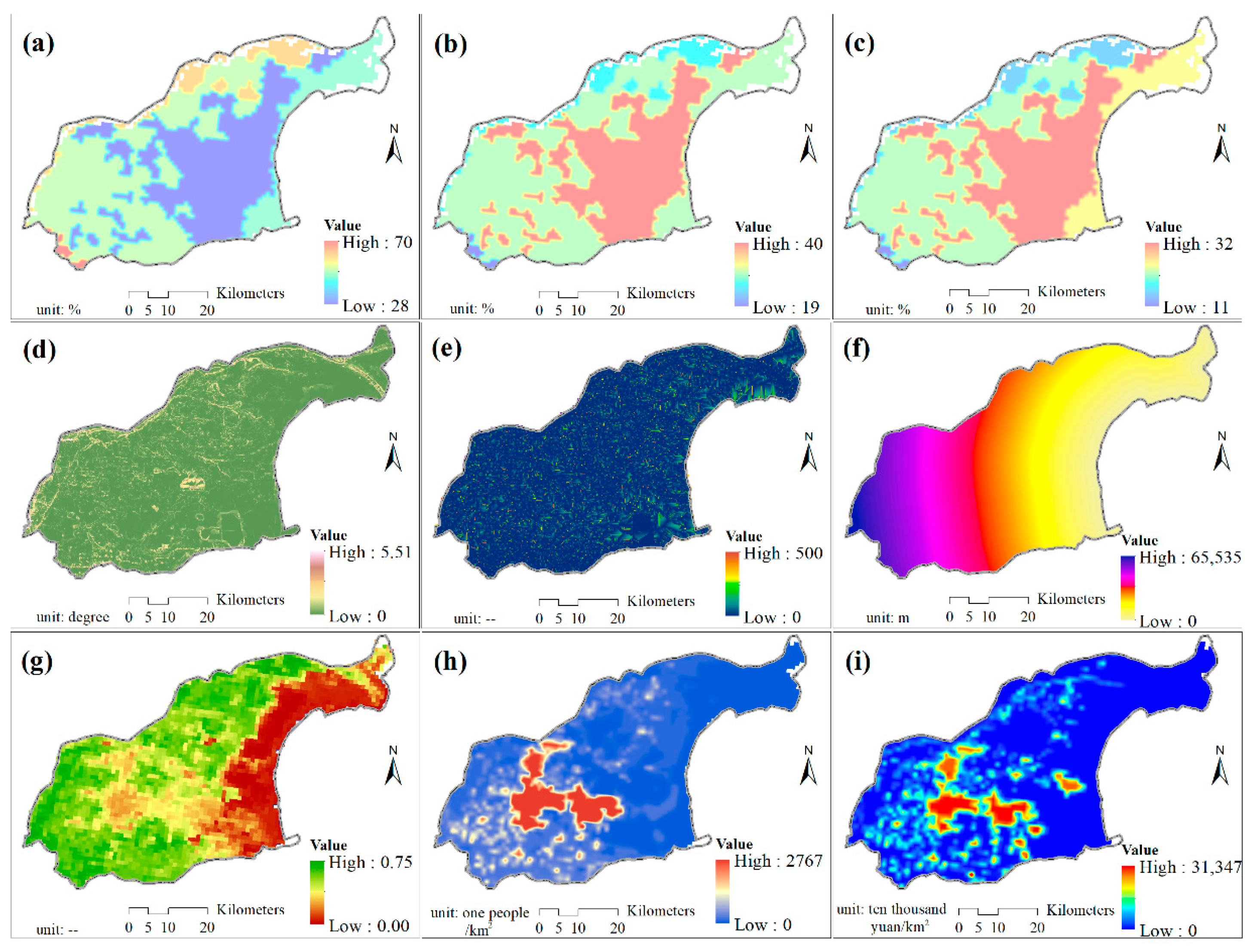
Relevant geographic grid layers were used to evaluate spatial heterogeneity. The auxiliary spatial data included (i) soil texture layers, consisting of the percentage data of sand, silt, and clay ratios (see Figure 2a–c), which were obtained from the Resource and Environment Science and Data Center of Chinese Academy of Sciences (RESDC) (http://www.resdc.cn/ (accessed on 29 August 2019)); (ii) a digital elevation model (DEM) (see Figure 1b), which was obtained from the Geospatial Data Cloud of China (http://www.gscloud.cn/ (accessed on 30 June 2009)). Additionally, we calculated the slope layer (see Figure 2d) and flow layer (see Figure 2e) based on DEM data; (iii) the annual average rainfall layers from 2011 to 2015( see Figure 1e); (iv) the monthly normalized difference vegetation index (NDVI) layers from June to October for 2015 to 2019, and we calculated the monthly and annual mean values (see Figure 2g); (v) the population distribution layer (see Figure 2h) and gross domestic product (GDP) distribution data (see Figure 2i), and the source data for (iii) to (v) were all collected from the RESDC website; and (vi) the distance from the sea (DS) layer (see Figure 1f), which was obtained as a result of this research. Then, we resampled the geographic data and obtained a 30-m resolution result.

2.3. Interpolation of Soil Sampling Data and Verification

We selected the interpolation method with maximum precision among ordinary kriging (OK), inverse distance weighted (IDW), geographically weighted regression (GWR), and geographically weighted regression kriging (GWRK), to obtain the spatial layers of SOM and STN.

2.3.1. Ordinary Kriging

OK is a commonly effective interpolation method that establishes a spatial statistical model based on the spatial autocorrelation between sampling sites to predict the surface [52,53] (see Equation (1)).
K ( x 0 ) = i = 1 n λ i K ( x i ) .
where K(x0) is the predicted value in the x0 point, K(xi) is the measured value of the known sample around x0, λi is the weight of the ith known soil sample, related to distance, spatial location, and layout, etc., and n is the amount of the known sample sites.

2.3.2. IDW

IDW plays a good interpolation role in the data spatialization, which assigns a larger weight to the closer sample according to the distance between the samples and predicted points and then performs a weighted average of the samples to obtain the predicted value [54] (see Equation (2)).
I ( x 0 ) = i = 1 n I ( x i ) ( d i ) p / i = 1 n 1 ( d i ) p .
where I(x0) is the predicted value in the x0 point, I(xi) is the measured data in the ith sample site, di is the distance between soil samples and the predicted point, and p is the power value of the weight.

2.3.3. GWR and GWRK

The GWR model is a spatially varying coefficient model attached to the additional concept of spatial location, the regression coefficients of which are determined by a function of the spatial location variable [55,56] (see Equation (3)). GWRK added the process of regression residual removal based on the GWR result, including a residual spatialization by the kriging method [57].
y i = β 0 ( u i , v i ) + j = 1 k β j ( u i , v i ) x i j + ε i .
where yi is the predicted value of the ith point, β0(ui, vi) is the intercept of the polynomial, βj(ui, vi) is the regression coefficient of the jth impact variable at the ith prediction point, which is a function of the location (ui, vi), Xij is the value of the jth impact variable at the ith point, and εi is the random error term.

2.3.4. Verification

We supplemented a cross-validation process [58,59,60] by evaluating the statistical mean error (ME) (Equation (4)), mean absolute error (MAE) (Equation (5)) and root mean squared error (RMSE) (Equation (6)) of the abovementioned interpolation methods to obtain the optimal spatial layers of SOM and STN.
ME = 1 m i = 1 m ( y i y i ) .
MAE = 1 m i = 1 m | y i y i |
RMSE = 1 m i = 1 m ( y i y i ) 2
where yi is the predicted value at the ith verification sample, while yi is the ith sampling value, and m is the number of verification samples; in this study, 10% of the soil samples were extracted. The smaller the values of ME, MAE, and RMSE, the higher the accuracy of the interpolation results.

2.4. Soil Nitrogen Loss Risk Index

Based on the RUSLE, we developed a soil total nitrogen loss risk index (SNLRI) to quantify the risk of soil nitrogen loss dominated by soil erosion. In the SNLRI, we applied the soil erodibility factor (K), slope factor (S), vegetation cover factor (V), and rainfall erosivity factor (R) in RUSLE and added a flow factor (F) [61] to comprehensively characterize the soil nitrogen loss risks [62]. However, the SNLRI calculates the nitrogen loss risk by normalizing each impact factor and superimposing them with weights (see Equation (7)).
SNLRI = i = 1 n f i × w i .
where 0 ≤ SNLRI ≤ 1 is the soil nitrogen loss risk index, 0 ≤ fi ≤ 1 is the soil loss contribution index of the ith influencing factor, n is the amount of the soil loss influencing factors, and wi corresponds to the weight.

2.4.1. Soil Erodibility Factor

In the RUSLE, the soil erodibility factor (K) characterizes soil loss from the soil content (soil sand, soil silt, soil clay, and soil organic carbon (SOC)) perspective (see Equation (8)); usually, a larger K value presents a stronger soil erosion risk [23,63,64]. However, the nitrogen in the soil surface is often dissolved in water and lost with the soil erosion process [65,66]. Therefore, the soil erodibility index (K) can present the soil nitrogen loss risk well.
K = { 0.2 + 0.3 × exp [ 0.0256 × S A N × ( 1 S I L 100 ) ] } × ( S I L C L A + S I L ) 0.3 × [ 1 0.25 × S O C S O C + exp ( 3.72 2.95 × S O C ) ] × { 1 0.7 × ( 1 S A N 100 ) ( 1 S A N 100 ) + exp [ 5.51 + 22.9 × ( 1 S A N 100 ) ] } .
where K is the soil erodibility index, t·h·MJ−1·mm−1. SAN is the soil sand content (%), SIL is the soil silt content (%), CLA is the soil clay content (%), and SOC is the soil organic carbon content (%). The SOC data is calculated by using a modulus of 0.58 based on the sampled SOM data (that is, SOC/SOM = 0.58) [67].

2.4.2. Slope Factor

Different terrain slopes usually show differentiated soil loss potential [68,69]. We applied the slope factor in the RUSLE (see Equation (9)) to quantify the slope contribution to the soil loss risk.
S = { 10.8 × sin θ + 0.03 , θ < 9 % 16.8 × sin θ 0.50 , 9 % θ 18 % 21.91 × sin θ 0.96 , θ > 18 % .
where S is the slope factor index and θ is the angle value at a grid scale.

2.4.3. Vegetation Coverage Factor

Terrestrial vegetation plays an initial role in soil and water conservation. Vegetation coverage may effectively reduce the soil nutrient loss caused by soil erosion [70]. However, the vegetation impact on soil loss can be properly quantified by the NDVI (see Equation (10)) [71].
V = exp [−(2 × NVDI)/(1 − NVDI)]
where V is the vegetation coverage factor index; the larger the value, the greater contribution to soil loss. NDVI is the mean monthly NDVI value in summer.

2.4.4. Hydraulic Erosivity Factors

In this study, we mainly considered two types of hydraulic influencing factors in the SNLRI, named the rainfall erosivity factor (R) and flow factor (F). Rainfall is the governing force for soil loss, and greater rainfall intensity usually corresponds to larger soil loss risks [24,72]. We applied the average annual rainfall from 2011 to 2015 to quantify the regional heterogeneity of rainfall erosivity. In addition to rainfall, the erosion effect of upstream incoming water on the soil surface also plays an important role in soil loss [73,74]. Therefore, we also applied the hydrological flow to calculate the F factor, presenting the hydrological promotion effect on soil loss during the runoff process. In this study, we used the range conversion method to normalize the R and F factors, and a larger rainfall or flow value corresponded to a larger contribution to the SNLRI.

2.4.5. Weight Determination and the SNLRI

In this study, we assessed the relative spatial risk distributions by using a normalized index. Therefore, the spatial variability in the influencing factors determined their heterogeneity contribution levels. For the overlay of risk factors, we used the spatial standard deviation (SD) of every factor layer to determine their weights (see Equation (11)). Then, we can obtain the final SNLRI distribution layer by comprehensively superimposing the five types of soil loss factors.
w i = σ i / i = 1 n σ i .
where wi is the weight of the ith soil loss influence factor, and σi represents the spatial standard deviation of the ith influence factor.

2.5. Anthropogenic Soil Nitrogen Net Replenishment Index

We proposed a simple soil nitrogen index to present the STN net supply to soil dominated by human activities, named the anthropogenic soil nitrogen net replenishment index (A-SNNRI). In the A-SNNRI, the STN replenishment mainly consists of the soil nitrogen variety and the soil loss part. However, we did not add other soil nitrogen losses, such as volatilization and transformation processes, which occurred at relatively low levels.

2.5.1. STN Change Index

STN change is a comprehensive result of soil nitrogen gains and losses within a certain temporal scale. We calculated the STN change index (SNCI) based on the variety of STN concentrations to present the replenishment possibility of soil nitrogen (see Equation (12)).
SNCI = ( STN a f t e r STN a f t e r ) M i n ( STN a f t e r STN a f t e r ) M a x ( STN a f t e r STN a f t e r ) M i n ( STN a f t e r STN a f t e r ) .
where 0 ≤ SNCI ≤ 1 is the STN change index; the larger value corresponds to the higher STN replenishment possibility. STNafter and STNbefore represent the STN concentration in October and June, respectively.

2.5.2. A-SNNRI

By weighting and superimposing the SNLRI and SNCI layers (Equation (13)), we can obtain the regional A-SNNRI result. For the weight, we also referenced the weight determination method based on the SD of the grid layer (see Equation (11)).
A - S N N R I = SNCI × w 1 + S N L R I × w 2 .
where 0 ≤ A-SNNRI ≤ 1 is the anthropogenic soil nitrogen net replenishment index; the larger the value, the larger the nitrogen supply capability is w1 and w2 are the weights of the SNCI and SNLRI, respectively.

2.6. Statistics

In this study, we implemented relevant geostatistical analysis and the overlay of grid layers under an ArcGIS 10.2 environment (Environmental Systems Research Institute, Redlands, WA, USA). For the spatial correlation analysis, we applied a resampling method to obtain the simulated samples based on ArcToolbox tools. However, the basic statistical analysis was based on SPSS 20 (International Business Machines Corporation, Armonk, NY, USA) and Excel 2016 (Microsoft, Redmond, WA, USA). The software mentioned above were all obtained from Institute of Geographic Sciences and Natural Resources Research, Chinese Academy of Sciences. In addition, the factor detector tool in Geodetector [75] (see Equation (14)) played a better role in the evaluation of spatial stratified heterogeneity and the correlation analysis of qualitative data.
q = 1 h = 1 L N h δ h 2 / N δ 2 .
where 0 ≤ q ≤ 1; the larger value indicates a stronger heterogeneity under the strata status and higher correlation with the qualitative data. h is the classification number of the qualitative spatial data (e.g., the land use layer). Nh and N are the unit numbers of zone h and the entire region, respectively. δ2h and δ2 correspond to the variances of zone h and the entire region.

3. Results

3.1. Spatiotemporal Distributions of STN and SOM

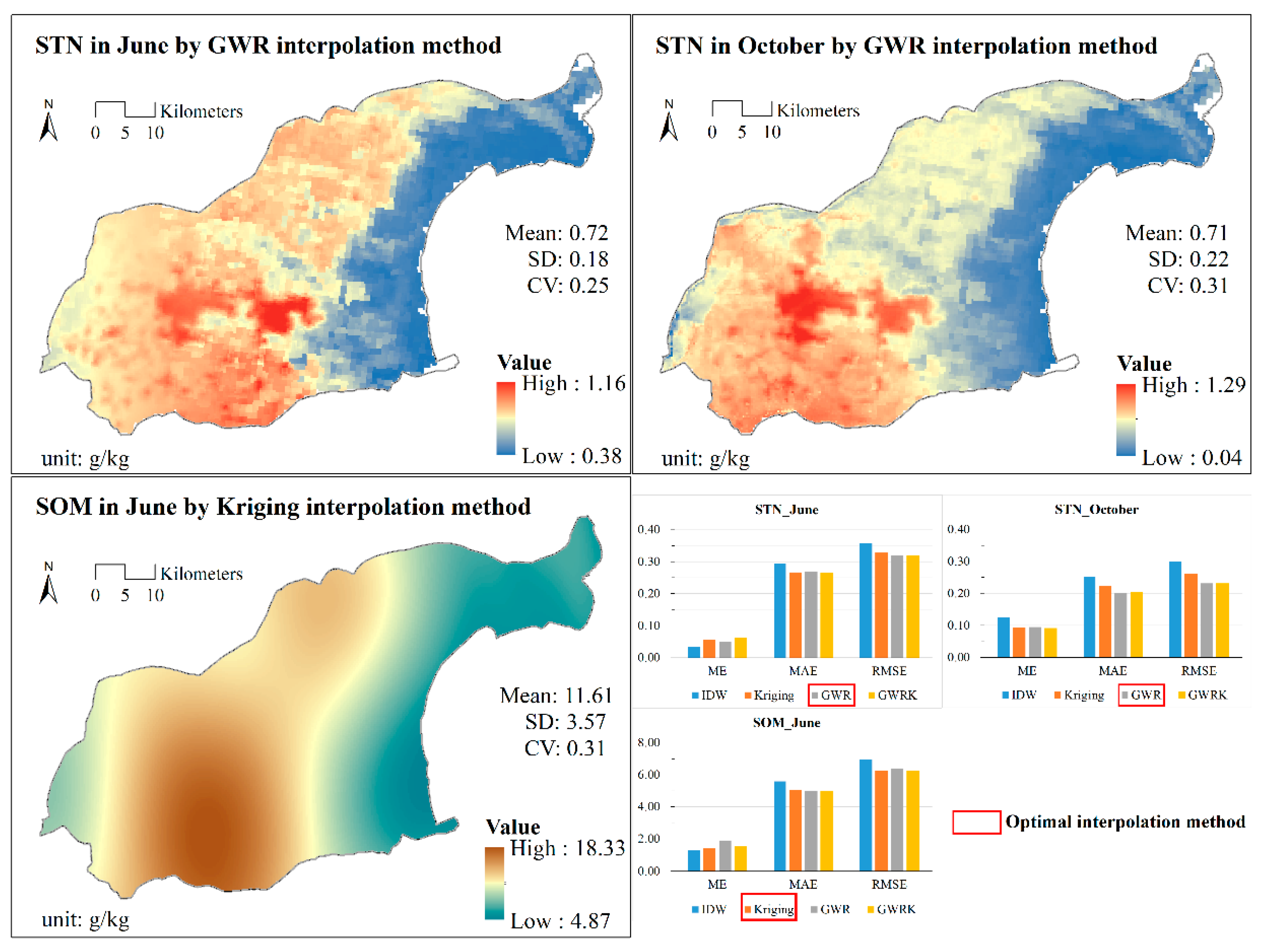
We obtained the spatial layers of STN in June and October 2020 and SOM in June by selecting the best interpolation results (see Figure 3). Then, we calculated the regional STN changes from June to October (see Figure 4). Moreover, the influences of environmental factors on soil indicators were analyzed (see Table 1).

3.1.1. STN and SOM Characteristics

We obtained the STN spatial layers for June and October 2020 by the GWR model and the SOM result for June with the kriging method (see Figure 3). In Figure 3, the STN concentrations in June and October presented consistent distributions in the study area. Lower values were distributed along the east coast and presented an increasing trend with increasing distance from the sea. The highest values of STN were in the main city of Dongying and the southwestern region. However, the mean STN values in June and October were 0.72 g/kg and 0.71 g/kg, respectively. In terms of SOM, there were distributions similar to those of STN; the east coast had lower concentrations, and the southwestern part had the highest value. Overall, the mean SOM value in June was 11.61 g/kg.

3.1.2. STN Change and Impact Factor Analysis

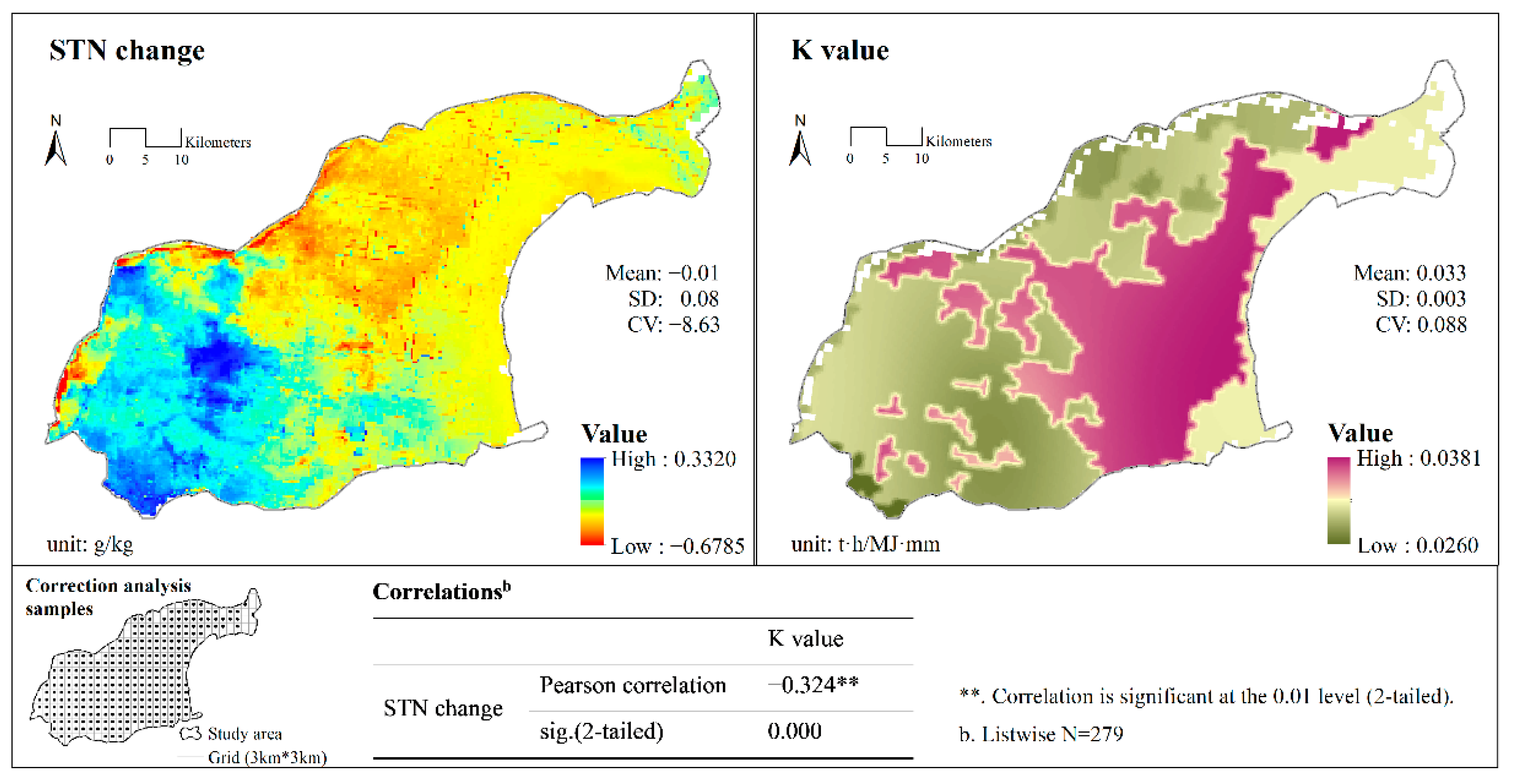
The spatial STN variety from June to October is shown in Figure 4. In the study area, the STN changes were balanced overall after the summer crop-growing season, with a regional mean value of −0.01 g/kg. However, the larger decreases in STN were mainly located in the northern area and the east coast. There were obvious STN increases in the main city and southwest.
From the land use perspective, overall, the STN distributions in June and October showed a consistent trend; that is, the mean STN concentration presented the order of urban villages > arable land > garden land > industrial and mining storage land > woodland > tidal flat land (see Figure 5a,b). In Figure 5c,d, the largest values of the summary STN change were also located in urban villages and arable land. However, the mean STN change in arable land was relatively low, and the larger values were mainly located in urban villages, industrial and mining storage land, and facility agricultural land.
In Table 1, we obtained the correlations between soil indicators and relevant environmental factors. The SPSS correlation analysis results of the STN influencing factors in June and October were also applied in the GWR model. In June, the STN distributions had significant positive correlations with the NDVI and population (p < 0.01), and the Pearson correlation coefficients were 0.32 and 0.25, respectively. The October STN presented significant positive correlations with the NDVI, DS, population, and elevation (p < 0.05), and the Pearson correlation coefficients were 0.34, 0.32, 0.23, and 0.21, respectively. In addition, the SOM in June presented significant positive correlations with the NDVI, population, and DS (p < 0.05), which presented correlation coefficients of 0.34, 0.26, and 0.20. However, the STN change had significant correlations with all the mentioned environmental factors (p < 0.05), and the coefficients with DS, rainfall, population, and elevation all exceeded 0.3. The silt and clay indicators both presented significant negative correlations with STN change. Moreover, the Geodetector analysis results showed that STN, SOM, and STN changes all presented significant correlations with land use (p < 0.01), and the q values of STN and SOM concentrations all exceeded 0.35.

3.2. Soil Nitrogen Loss Risks in the YRD

To present the heterogeneity of STN loss risks, we applied the RUSLE to evaluate soil erodibility and soil loss. Then, based on land use, the correlations between soil loss and STN variety were analyzed.

3.2.1. Distribution of Soil Erodibility

In Figure 4, the mean K value of the study area was 0.033 t·h·MJ−1·mm−1, which was relatively high. This phenomenon occurred mainly because the land-forming soil of the YRD came from the Loess Plateau, and there was higher land exposure in the study area [50]. In terms of spatial distributions, there had higher soil erodibility on the east coast, and the highest K values were mainly distributed in the Guangli River estuary and its upward-extending area in the southeast.

3.2.2. SNLRI Analysis

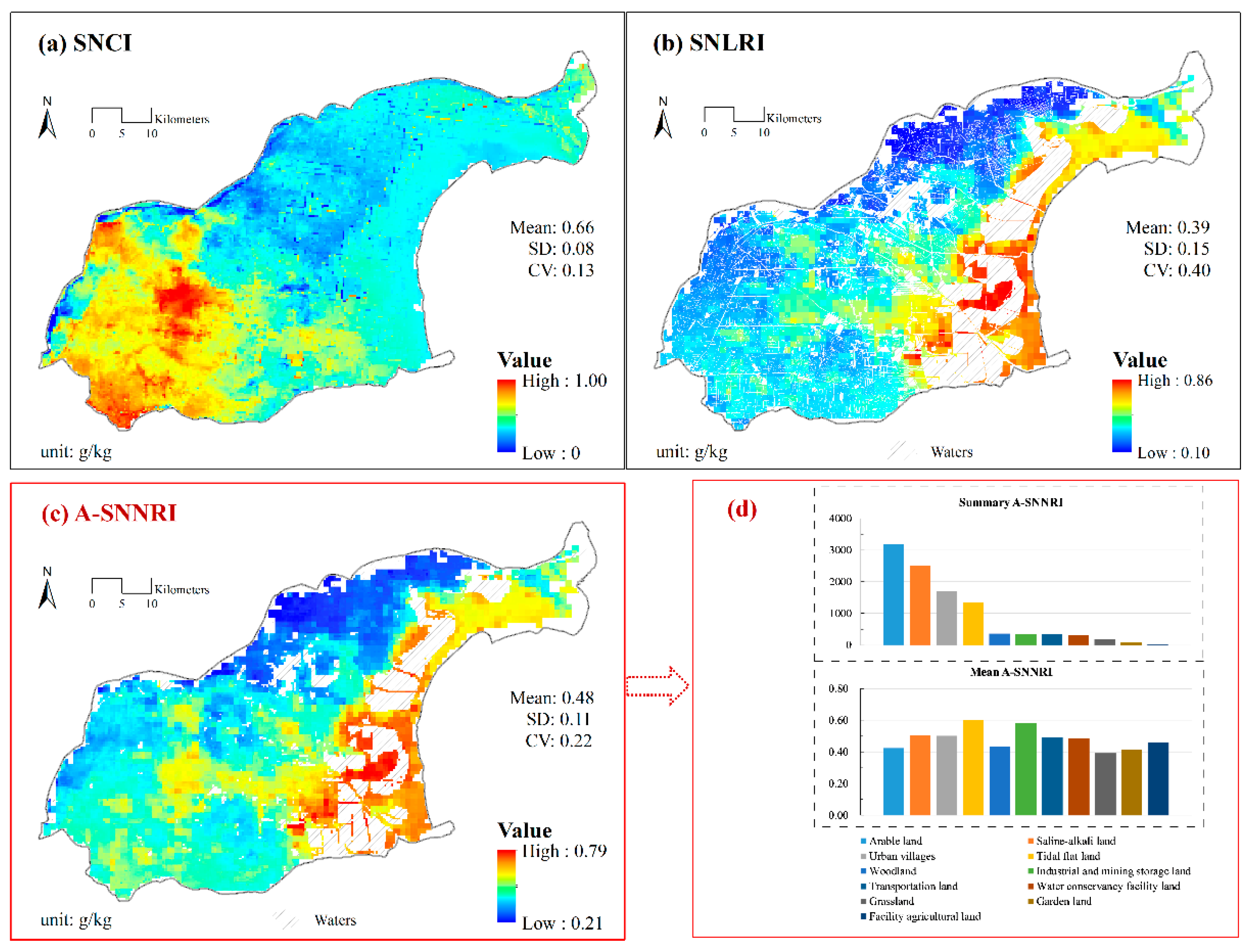
We obtained the risk contributions of the five soil loss factors according to the RUSLE (see Figure 6). Then, we calculated the spatial SD (σ) values of the normalized layers of soil loss factors and generated the overlaying weights to the SNLRI (see Equation (11)). The SDs of the five soil loss factors presented the order of V > K > R > F > S, which was also the order of their weights. In the study area, vegetation cover, soil erodibility, and rainfall erosivity were the main leading factors affecting the spatial heterogeneity of soil loss. Figure 7b presents the final SNLRI calculated result, where the higher SNLRIs are mainly distributed along the east coast, the main city of Dongying, and the Guangli River.

3.2.3. Soil Loss Influence on STN Change

In Figure 4, the soil erodibility (K) had a significant negative correlation with the STN change, and the correlation coefficient was 0.32 (p < 0.01). Moreover, we obtained the correlation between the summary soil loss risks and the total STN changes based on the land use divisions (see Figure 5e,f). For the land use statistical results, we can conclude that the STN change was significantly negatively correlated with the summary soil loss risk, with a determination coefficient (R2) of 0.82, except for the land use types of urban villages and arable land. Although the urban villages and the arable land had higher soil loss risks, they also attached larger increments of STN.

3.3. Spatial Distributions of A-SNNRI

We obtained the A-SNNRI layer by applying Equation 13 and analysed the index distribution in different land uses (see Figure 7c,d). In this study, based on the spatial SD and Equation (11), the overlay weights of the SNCI and SNLRI for presenting the final A-SNNRI layer were 0.33 and 0.67, respectively. In Figure 7c, the spatial A-SNNRIs presented higher values on the east coast and the southeast, especially for the main city of Dongying. For the land use statistics, the higher values of summary A-SNNRIs were mainly located in arable land, saline-alkali land, and urban villages, while the larger mean A-SNNRIs were distributed in tidal flat land, industrial and mining storage land, saline-alkali land and urban villages (see Figure 7d). Although the summary A-SNNRI in arable land was the largest, the mean value was relatively low. However, the summary and mean A-SNNRIs of urban villages and saline-alkali land all presented higher values in the study area.

4. Discussion

4.1. Influences of Human Activities on STN Status

4.1.1. Influence of Land Use on STN Distribution

There were higher STN values on the east coast in Figure 3 and higher values in agricultural land uses in Figure 5. The spatial distribution characteristics of STN and SOM were mainly due to seawater intrusion and agricultural development [51]. In this case, the soil fertility in the sea-proximity areas was poorer, and the crop planting was concentrated in the inland areas. Agriculture and human activities had a certain increasing effect on the STN and SOM concentrations.

4.1.2. Anthropogenic STN Supplement Analysis

In estuarine deltas, human activities usually have greater influence on the STN status and variety [76]. We selected the population and GDP indicators for presenting the intensity of human activity and used the DS indicator to evaluate the influence of sea distribution in coastal areas. Then, we implemented the correlation analysis between the calculated A-SNNRIs and the spatial data of population, GDP and DS in the YRD (see Table 2). The A-SNNRI showed significant positive correlations with population and GDP (p < 0.05) but presented significant negative correlations with DS (p < 0.01). To some extent, population concentration and socioeconomic development promote the flow of nitrogen to the soil. With the development of human society, the amount of nitrogen supplied to the soil by humans is generally greater than the land consumption, resulting in a net increase in soil nitrogen. In the YRD, the STN concentrations, STN increases and A-SNNRIs in urban villages were all relatively high. Although the coastal soil is poor, there is also a large proportion of arable land in the YRD. In this case, to obtain a higher land yield, people tend to add a larger amount of nitrogen to the soil to supplement the growth of crops [77]. However, due to the constraints of soil parent material and environmental conditions, future nitrogen replenishment to soil in arable land is not optimistic [78,79]. In this study, the mean STN concentration increases in arable land were relatively low. In addition, the A-SNNRIs of saline-alkali land were relatively high, which might be related to the saline-alkali soil improvement activities in this region [80]. In contrast, the DS had a certain negative effect on the A-SNNRIs (p < 0.01). We maintained that this is closely related to the strong sea–land interactions. In this case, the proximity to the sea results in poorer soil fertility, resulting in greater anthropogenic nitrogen resupply. Otherwise, according to the survey data of this study, there was a large proportion of aquaculture and other nonagricultural industries near the coast, which significantly supplements the soil nitrogen [81,82].

4.2. A-SNNRI Application in the Control of Coastal Nonpoint Source Pollution

Compared with other terrestrial areas, the discharge of terrestrial pollutants into the sea in coastal areas is more direct and larger [5,83]. Therefore, coastal areas are usually the key sources of marine pollution, and it is necessary to accurately grasp the spatial locations of the main source region [84,85]. However, the process of terrestrial pollutants generated by human activities entering water bodies as nonpoint source pollution through water and soil processes is complicated. It is difficult to spatially quantify the specific pollutant supplements of human activities to the soil. Therefore, this research focuses on the soil loss potential and the changes in soil pollutant content to infer an A-SNNRI and evaluate the spatial heterogeneity of soil nitrogen replenishment dominated by human activities. Then, based on the A-SNNRI, we can obtain the spatial distributions of the nitrogen export risks and the key influencing factors. The research methods and results presented in this study may provide a good reference in the spatial management and control strategies for coastal nonpoint source pollution.
In this paper, the SNLRIs were relatively high on the east coast and in the main city of Dongying, corresponding to higher soil nitrogen loss risks. For the analysis of the distribution of soil loss influencing factors, we may obtain the main pollutant emission influencing factors of the vegetation coverage, soil erodibility, and rainfall. Therefore, we can conclude that it is an initial step to add the density of coastal vegetation planting and increase offshore soil and water conservation effects. Additionally, in the study area, to control the discharge of nitrogen nonpoint source pollution into the sea, we must strengthen farmland planting management and reduce nitrogen fertilizer inputs in the southwest. However, we should also consider the summer crop growing season as the key period for the control of the into-sea nonpoint source pollution.

4.3. Limitations

In this study, there were still some limitations in the data setting and methods. From the data limitation perspective, there was a mismatch in the temporal scale of the research data. In this study, due to the limited data involved in sampling and experiments, some of the auxiliary geographic data came from the existing research results. The land use, soil texture, rainfall, and NDVI data were not displayed during the sampling period. In addition, the spatial resolution of some spatial data needs to be improved. From the method limitation perspective, in this study, we mainly focused on the soil erosion processes that had the greatest impacts on the nitrogen loss in the soil surface but did not include the vertical migration of soil nitrogen and other loss influences. In addition, compared with the inherent nitrogen content of the original soil, the nitrogen supplied by human activity in other forms might present a differentiated loss law when soil erosion occurs. However, this study used the RUSLE to uniformly analyse the loss risks of these two types of nitrogen formats. We mainly intended to present a generalized risk index of the soil nitrogen net replenishment influenced by human activities and quantify its spatial heterogeneity.

5. Conclusions

In this study, based on the actual soil nitrogen status and soil loss risk, we established a simple method to evaluate the soil nitrogen net replenishment risk dominated by human activities. A case study in the YRD showed that the A-SNNRI could present the supply intensity to soil nitrogen well. The main conclusions are described as follows.
(i)
In the study area, the STN and SOM presented consistent spatial distributions, with lower values on the east coast and the highest values in the southwest and the main city of Dongying. The mean values of STN and SOM were 0.7 g/kg (June and October) and 11.6 g/kg (June), respectively. The larger STN decreases were in the northern area and the east coast, while the STN increases were mainly in the main city and the southwest. Urban villages and arable land held the largest mean STNs and summary changes. Population and land use presented significant influences on STN status. However, sea proximity was a negative factor for the STN content and variety.
(ii)
The soil erodibility was relatively high, and the K value was 0.033 t·h·MJ−1·mm−1. Higher soil loss risks were mainly located on the coast, the larger estuaries of the southeast, and the main city of Dongying. The contributions of influencing factors to the SNLRI showed the order of V > K > R > F > S. There were significant negative correlations between the STN changes and the K values. Moreover, except for urban villages and arable land, other land uses showed that the summary STN changes had significant negative correlations with soil loss.
(iii)
Higher A-SNNRIs were mainly located on the east coast, the southeast region, and the main city of Dongying, which also had the largest soil loss risks. The contribution weights of SNCI and SNLRI to the A-SNNRI were 0.33 and 0.67, respectively. Larger values of the summary A-SNNRIs were found in arable land, saline-alkali land, and urban villages, while the mean A-SNNRI of arable land was relatively low. However, tidal flat land and industrial and mining storage land had the largest mean A-SNNRIs. The distributions of population and socioeconomic activities presented significant influences on the A-SNNRIs. In the YRD, the pollution risk sources of STN were mainly in urban villages, agriculture, industry, and aquaculture.
(iv)
In coastal areas, there are often settlements of human life and socioeconomic production, which are also the main sources of marine pollution. However, due to differences in the regional natural conditions and the development of the social economy, the impacts of such human activities on coastal pollution often present spatial heterogeneity. Therefore, when formulating corresponding land-source management and control strategies for marine pollution in coastal areas, we should determine pollutant sources from the human behaviour perspective in a spatially specific way.

Author Contributions

Design of the research: Y.W., G.L., C.H. and Z.Z.; Data collection: Y.W., G.L., C.H., H.L. and Q.L.; Data analysis and interpretation: Y.W.; Manuscript draft and revision: Y.W., G.L. and Z.Z. All authors have read and agreed to the published version of the manuscript.

Funding

This research was supported by the Strategic Priority Research Program of Chinese Academy of Sciences, grant number XDA23050101, and the National Natural Science Foundation of China, grant number 42001227.

Institutional Review Board Statement

Not applicable.

Informed Consent Statement

Not applicable.

Data Availability Statement

All data presented in this paper are available from the first author of Y.W. ([email protected]).

Conflicts of Interest

The authors declare that they have no known competing financial interests or personal relationships that could have appeared to influence the work reported in this paper.

References

  1. Shao, Q.; Guo, J.; Kang, P. Environmental response to growth in the marine economy and urbanization: A heterogeneity analysis of 11 Chinese coastal regions using a panel vector autoregressive model. Mar. Policy 2021, 124, 104350. [Google Scholar] [CrossRef]
  2. Cao, W.; Wong, M.H. Current status of coastal zone issues and management in China: A review. Environ. Int. 2007, 33, 985–992. [Google Scholar] [CrossRef]
  3. Pan, K.; Wang, W.X. Trace metal contamination in estuarine and coastal environments in China. Sci. Total Environ. 2012, 421–422, 3–16. [Google Scholar] [CrossRef] [PubMed]
  4. Niu, X.Y.; Wang, Y.H.; Yang, H.; Zheng, J.W.; Zou, J.; Xu, M.N.; Wu, S.S.; Xie, B. Effect of Land Use on Soil Erosion and Nutrients in Dianchi Lake Watershed, China. Pedosphere 2015, 25, 103–111. [Google Scholar] [CrossRef]
  5. Huang, J.; Li, Q.; Huang, L.; Zhang, Z.; Mu, J.; Huang, Y. Watershed-scale evaluation for land-based nonpoint source nutrients management in the Bohai Sea Bay, China. Ocean Coast. Manag. 2013, 71, 314–325. [Google Scholar] [CrossRef]
  6. Meng, Q.; Fu, B.; Tang, X.; Ren, H. Effects of land use on phosphorus loss in the hilly area of the Loess Plateau, China. Environ. Monit. Assess. 2008, 139, 195–204. [Google Scholar] [CrossRef]
  7. Fang, S.; Pang, H.; Dai, X. Soil nitrogen and phosphorous dynamics by in situ soil experiments along an urban-rural gradient in Shanghai, China. Environ. Sci. Pollut. Res. 2019, 26, 31026–31037. [Google Scholar] [CrossRef]
  8. Sun, B.; Gu, L.; Bao, L.; Zhang, S.; Wei, Y.; Bai, Z.; Zhuang, G.; Zhuang, X. Application of biofertilizer containing Bacillus subtilis reduced the nitrogen loss in agricultural soil. Soil Biol. Biochem. 2020, 148, 107911. [Google Scholar] [CrossRef]
  9. Özbek, F.Ş.; Leip, A. Estimating the gross nitrogen budget under soil nitrogen stock changes: A case study for Turkey. Agric. Ecosyst. Environ. 2015, 205, 48–56. [Google Scholar] [CrossRef]
  10. Sitters, J.; Wubs, E.R.J.; Bakker, E.S.; Crowther, T.W.; Adler, P.B.; Bagchi, S.; Bakker, J.D.; Biederman, L.; Borer, E.T.; Cleland, E.E.; et al. Nutrient availability controls the impact of mammalian herbivores on soil carbon and nitrogen pools in grasslands. Glob. Chang. Biol. 2020, 26, 2060–2071. [Google Scholar] [CrossRef] [Green Version]
  11. Lu, Y.; Silveira, M.L.; O’Connor, G.A.; Vendramini, J.M.B.; Erickson, J.E.; Li, Y.C. Assessing the impacts of biochar and fertilizer management strategies on N and P balances in subtropical pastures. Geoderma 2021, 394, 115038. [Google Scholar] [CrossRef]
  12. An, S.; Zheng, F.; Zhang, F.; Van Pelt, S.; Hamer, U.; Makeschin, F. Soil quality degradation processes along a deforestation chronosequence in the Ziwuling area, China. Catena 2008, 75, 248–256. [Google Scholar] [CrossRef]
  13. Antikainen, R.; Lemola, R.; Nousiainen, J.I.; Sokka, L.; Esala, M.; Huhtanen, P.; Rekolainen, S. Stocks and flows of nitrogen and phosphorus in the Finnish food production and consumption system. Agric. Ecosyst. Environ. 2005, 107, 287–305. [Google Scholar] [CrossRef]
  14. Yang, Y.H.; Ma, W.H.; Mohammat, A.; Fang, J.Y. Storage, Patterns and Controls of Soil Nitrogen in China. Pedosphere 2007, 17, 776–785. [Google Scholar] [CrossRef]
  15. Lewis, D.B.; Castellano, M.J.; Kaye, J.P. Forest succession, soil carbon accumulation, and rapid nitrogen storage in poorly remineralized soil organic matter. Ecology 2014, 95, 2687–2693. [Google Scholar] [CrossRef]
  16. Tian, L.; Zhao, L.; Wu, X.; Hu, G.; Fang, H.; Zhao, Y.; Sheng, Y.; Chen, J.; Wu, J.; Li, W.; et al. Variations in soil nutrient availability across Tibetan grassland from the 1980s to 2010s. Geoderma 2019, 338, 197–205. [Google Scholar] [CrossRef]
  17. Xie, M.; Zhao, L.; Wu, X.; Tian, L.; Yue, G.; Zhou, H.; Wu, Z. Seasonal variations of nitrogen in permafrost-affected soils of the Qinghai-Tibetan Plateau. Catena 2020, 195, 104793. [Google Scholar] [CrossRef]
  18. Maury, S.; Gholkar, M.; Jadhav, A.; Rane, N. Geophysical evaluation of soils and soil loss estimation in a semiarid region of Maharashtra using revised universal soil loss equation (RUSLE) and GIS methods. Environ. Earth Sci. 2019, 78, 144. [Google Scholar] [CrossRef]
  19. Li, Y.; Liu, C.; Yuan, X. Spatiotemporal features of soil and water loss in Three Gorges Reservoir Area of Chongqing. J. Geogr. Sci. 2009, 19, 81–94. [Google Scholar] [CrossRef]
  20. Abdo, H.; Salloum, J. Mapping the soil loss in Marqya basin: Syria using RUSLE model in GIS and RS techniques. Environ. Earth Sci. 2017, 76, 114. [Google Scholar] [CrossRef]
  21. Schürz, C.; Mehdi, B.; Kiesel, J.; Schulz, K.; Herrnegger, M. A systematic assessment of uncertainties in large-scale soil loss estimation from different representations of USLE input factors-a case study for Kenya and Uganda. Hydrol. Earth Syst. Sci. 2020, 24, 4463–4489. [Google Scholar] [CrossRef]
  22. Jin, F.; Yang, W.; Fu, J.; Li, Z. Effects of vegetation and climate on the changes of soil erosion in the Loess Plateau of China. Sci. Total Environ. 2021, 773, 145514. [Google Scholar] [CrossRef] [PubMed]
  23. Chen, H.; Oguchi, T.; Wu, P. Assessment for soil loss by using a scheme of alterative sub-models based on the RUSLE in a Karst Basin of Southwest China. J. Integr. Agric. 2017, 16, 377–388. [Google Scholar] [CrossRef] [Green Version]
  24. Phinzi, K.; Ngetar, N.S. The assessment of water-borne erosion at catchment level using GIS-based RUSLE and remote sensing: A review. Int. Soil Water Conserv. Res. 2019, 7, 27–46. [Google Scholar] [CrossRef]
  25. Feng, T.; Chen, H.; Polyakov, V.O.; Wang, K.; Zhang, X.; Zhang, W. Soil erosion rates in two karst peak-cluster depression basins of northwest Guangxi, China: Comparison of the RUSLE model with 137Cs measurements. Geomorphology 2016, 253, 217–224. [Google Scholar] [CrossRef]
  26. Kulimushi, L.C.; Choudhari, P.; Mubalama, L.K.; Banswe, G.T. GIS and remote sensing-based assessment of soil erosion risk using RUSLE model in South-Kivu province, eastern, Democratic Republic of Congo. Geomat. Nat. Hazards Risk 2021, 12, 961–987. [Google Scholar] [CrossRef]
  27. De Santos Loureiro, N.; De Azevedo Coutinho, M. A new procedure to estimate the RUSLE EI30 index, based on monthly rainfall data and applied to the Algarve region, Portugal. J. Hydrol. 2001, 250, 12–18. [Google Scholar] [CrossRef]
  28. Chi, Y.; Shi, H.; Zheng, W.; Sun, J.; Fu, Z. Spatiotemporal characteristics and ecological effects of the human interference index of the Yellow River Delta in the last 30 years. Ecol. Indic. 2018, 89, 880–892. [Google Scholar] [CrossRef]
  29. Chi, Y.; Zheng, W.; Shi, H.; Sun, J.; Fu, Z. Spatial heterogeneity of estuarine wetland ecosystem health influenced by complex natural and anthropogenic factors. Sci. Total Environ. 2018, 634, 1445–1462. [Google Scholar] [CrossRef] [Green Version]
  30. Yi, L.; Yu, Z.; Qian, J.; Kobuliev, M.; Chen, C.; Xing, X. Evaluation of the heterogeneity in the intensity of human interference on urbanized coastal ecosystems: Shenzhen (China) as a case study. Ecol. Indic. 2021, 122, 107243. [Google Scholar] [CrossRef]
  31. Lin, C.Y.; Lin, W.T.; Chou, W.C. Soil erosion prediction and sediment yield estimation: The Taiwan experience. Soil Tillage Res. 2002, 68, 143–152. [Google Scholar] [CrossRef]
  32. Dong, J.; Zhou, K.; Jiang, P.; Wu, J.; Fu, W. Revealing horizontal and vertical variation of soil organic carbon, soil total nitrogen and C:N ratio in subtropical forests of southeastern China. J. Environ. Manag. 2021, 289, 112483. [Google Scholar] [CrossRef] [PubMed]
  33. Jelokhani-Niaraki, M.; Sadeghi-Niaraki, A.; Choi, S.M. Semantic interoperability of GIS and MCDA tools for environmental assessment and decision making. Environ. Model. Softw. 2018, 100, 104–122. [Google Scholar] [CrossRef]
  34. Prasannakumar, V.; Vijith, H.; Abinod, S.; Geetha, N. Estimation of soil erosion risk within a small mountainous sub-watershed in Kerala, India, using Revised Universal Soil Loss Equation (RUSLE) and geo-information technology. Geosci. Front. 2012, 3, 209–215. [Google Scholar] [CrossRef] [Green Version]
  35. Jayanthi, M.; Duraisamy, M.; Thirumurthy, S.; Samynathan, M.; Kabiraj, S.; Manimaran, K.; Muralidhar, M. Ecosystem characteristics and environmental regulations based geospatial planning for sustainable aquaculture development. Land Degrad. Dev. 2020, 31, 2430–2445. [Google Scholar] [CrossRef]
  36. Pan, X.; Tang, J.; Tian, C.; Li, J.; Zhang, G. Short- and medium-chain chlorinated paraffins in sediments from the Laizhou Bay area, North China: Implications for transportation from rivers to marine environment. Environ. Pollut. 2018, 243, 1460–1468. [Google Scholar] [CrossRef]
  37. Pan, X.; Tang, J.; Chen, Y.; Li, J.; Zhang, G. Polychlorinated naphthalenes (PCNs) in riverine and marine sediments of the Laizhou Bay area, North China. Environ. Pollut. 2011, 159, 3515–3521. [Google Scholar] [CrossRef] [Green Version]
  38. Zhang, R.; Zhang, G.; Zheng, Q.; Tang, J.; Chen, Y.; Xu, W.; Zou, Y.; Chen, X. Occurrence and risks of antibiotics in the Laizhou Bay, China: Impacts of river discharge. Ecotoxicol. Environ. Saf. 2012, 80, 208–215. [Google Scholar] [CrossRef]
  39. Song, D.; Gao, Z.; Zhang, H.; Xu, F.; Zheng, X.; Ai, J.; Hu, X.; Huang, G.; Zhang, H. GIS-based health assessment of the marine ecosystem in Laizhou Bay, China. Mar. Pollut. Bull. 2017, 125, 242–249. [Google Scholar] [CrossRef]
  40. Zhuang, W.; Gao, X. Distributions, sources and ecological risk assessment of arsenic and mercury in the surface sediments of the southwestern coastal Laizhou Bay, Bohai Sea. Mar. Pollut. Bull. 2015, 99, 320–327. [Google Scholar] [CrossRef]
  41. Gan, Y.; Huang, X.; Li, S.; Liu, N.; Li, Y.C.; Freidenreich, A.; Wang, W.; Wang, R.; Dai, J. Source quantification and potential risk of mercury, cadmium, arsenic, lead, and chromium in farmland soils of Yellow River Delta. J. Clean. Prod. 2019, 221, 98–107. [Google Scholar] [CrossRef]
  42. Hu, N.J.; Huang, P.; Liu, J.H.; Shi, X.F.; Ma, D.Y.; Zhu, A.M.; Zhang, J.; Zhang, H.; He, L.H. Tracking lead origin in the Yellow River Estuary and nearby Bohai Sea based on its isotopic composition. Estuar. Coast. Shelf Sci. 2015, 163, 99–107. [Google Scholar] [CrossRef]
  43. Yuan, H.; Li, T.; Ding, X.; Zhao, G.; Ye, S. Distribution, sources and potential toxicological significance of polycyclic aromatic hydrocarbons (PAHs) in surface soils of the Yellow River Delta, China. Mar. Pollut. Bull. 2014, 83, 258–264. [Google Scholar] [CrossRef] [PubMed]
  44. Xu, X.; Chen, Z.; Feng, Z. From natural driving to artificial intervention: Changes of the Yellow River estuary and delta development. Ocean Coast. Manag. 2019, 174, 63–70. [Google Scholar] [CrossRef]
  45. Cui, B.L.; Li, X.Y. Coastline change of the Yellow River estuary and its response to the sediment and runoff (1976–2005). Geomorphology 2011, 127, 32–40. [Google Scholar] [CrossRef]
  46. Chu, Z.X.; Sun, X.G.; Zhai, S.K.; Xu, K.H. Changing pattern of accretion/erosion of the modern Yellow River (Huanghe) subaerial delta, China: Based on remote sensing images. Mar. Geol. 2006, 227, 13–30. [Google Scholar] [CrossRef]
  47. Xia, J.; Ren, R.; Chen, Y.; Sun, J.; Zhao, X.; Zhang, S. Multifractal characteristics of soil particle distribution under different vegetation types in the Yellow River Delta chenier of China. Geoderma 2020, 368, 114311. [Google Scholar] [CrossRef]
  48. Qin, H.; Chen, F.; Liu, Y. Study on wave-influenced resistance to erosion of silty soil in Huanghe (Yellow) River Delta. Acta Oceanol. Sin. 2010, 29, 53–57. [Google Scholar] [CrossRef]
  49. Gao, P.; Wang, Y.; Li, P.; Zhao, G.; Sun, W.; Mu, X. Land degradation changes in the Yellow River Delta and its response to the streamflow-sediment fluxes since 1976. Land Degrad. Dev. 2018, 29, 3212–3220. [Google Scholar] [CrossRef]
  50. Wang, Y.; Liu, G.; Zhao, Z.; Wu, C.; Yu, B. Using soil erosion to locate nonpoint source pollution risks in coastal zones: A case study in the Yellow River Delta, China. Environ. Pollut. 2021, 283, 117117. [Google Scholar] [CrossRef]
  51. Wang, Y.; Liu, G.; Zhao, Z. Spatial heterogeneity of soil fertility in coastal zones: A case study of the Yellow River Delta, China. J. Soils Sediments 2021, 21, 1826–1839. [Google Scholar] [CrossRef]
  52. Radočaj, D.; Jurišić, M.; Antonić, O. Determination of soil C:N suitability zones for organic farming using an unsupervised classification in eastern Croatia. Ecol. Indic. 2021, 123, 107382. [Google Scholar] [CrossRef]
  53. Zhong, X.; Kealy, A.; Duckham, M. Stream Kriging: Incremental and recursive ordinary Kriging over spatiotemporal data streams. Comput. Geosci. 2016, 90, 134–143. [Google Scholar] [CrossRef]
  54. Guan, F.; Xia, M.; Tang, X.; Fan, S. Spatial variability of soil nitrogen, phosphorus and potassium contents in Moso bamboo forests in Yong’an City, China. Catena 2017, 150, 161–172. [Google Scholar] [CrossRef]
  55. Wang, K.; Zhang, C.; Li, W. Predictive mapping of soil total nitrogen at a regional scale: A comparison between geographically weighted regression and cokriging. Appl. Geogr. 2013, 42, 73–85. [Google Scholar] [CrossRef]
  56. Wang, S.; Zhuang, Q.; Jin, X.; Yang, Z.; Liu, H. Predicting soil organic carbon and soil nitrogen stocks in topsoil of forest ecosystems in Northeastern China using remote sensing data. Remote Sens. 2020, 12, 1115. [Google Scholar] [CrossRef] [Green Version]
  57. Wang, Y.; Xiao, Z.; Aurangzeib, M.; Zhang, X.; Zhang, S. Effects of freeze-thaw cycles on the spatial distribution of soil total nitrogen using a geographically weighted regression kriging method. Sci. Total Environ. 2021, 763, 142993. [Google Scholar] [CrossRef]
  58. Xie, Y.; Chen, T.B.; Lei, M.; Yang, J.; Guo, Q.J.; Song, B.; Zhou, X.Y. Spatial distribution of soil heavy metal pollution estimated by different interpolation methods: Accuracy and uncertainty analysis. Chemosphere 2011, 82, 468–476. [Google Scholar] [CrossRef]
  59. Gao, L.; Shao, M. The interpolation accuracy for seven soil properties at various sampling scales on the Loess Plateau, China. J. Soils Sediments 2012, 12, 128–142. [Google Scholar] [CrossRef]
  60. Wu, C.; Liu, G.; Huang, C. Prediction of soil salinity in the Yellow River Delta using geographically weighted regression. Arch. Agron. Soil Sci. 2017, 63, 928–941. [Google Scholar] [CrossRef]
  61. Gao, G.Y.; Fu, B.J.; Lü, Y.H.; Liu, Y.; Wang, S.; Zhou, J. Coupling the modified SCS-CN and RUSLE models to simulate hydrological effects of restoring vegetation in the Loess Plateau of China. Hydrol. Earth Syst. Sci. 2012, 16, 2347–2364. [Google Scholar] [CrossRef] [Green Version]
  62. Huo, J.; Liu, C.; Yu, X.; Chen, L.; Zheng, W.; Yang, Y.; Yin, C. Direct and indirect effects of rainfall and vegetation coverage on runoff, soil loss, and nutrient loss in a semi-humid climate. Hydrol. Process. 2021, 35, e13985. [Google Scholar] [CrossRef]
  63. Huang, F.; Chen, J.; Yao, C.; Chang, Z.; Jiang, Q.; Li, S.; Guo, Z. SUSLE: A slope and seasonal rainfall-based RUSLE model for regional quantitative prediction of soil erosion. Bull. Eng. Geol. Environ. 2020, 79, 5213–5228. [Google Scholar] [CrossRef]
  64. Zhang, L.; Bai, K.Z.; Wang, M.J.; Karthikeyan, R. Basin-scale spatial soil erosion variability: Pingshuo opencast mine site in Shanxi Province, Loess Plateau of China. Nat. Hazards 2016, 80, 1213–1230. [Google Scholar] [CrossRef]
  65. Mihara, M.; Yamamoto, N.; Ueno, T. Application of USLE for the prediction of nutrient losses in soil erosion processes. Paddy Water Environ. 2005, 3, 111–119. [Google Scholar] [CrossRef]
  66. Teixeira, P.C.; Misra, R.K. Measurement and prediction of nitrogen loss by simulated erosion events on cultivated forest soils of contrasting structure. Soil Tillage Res. 2005, 83, 204–217. [Google Scholar] [CrossRef]
  67. Ezzaouini, M.A.; Mahé, G.; Kacimi, I.; Zerouali, A. Comparison of the MUSLE model and two years of solid transport measurement, in the Bouregreg Basin, and impact on the sedimentation in the Sidi Mohamed Ben Abdellah Reservoir, Morocco. Water 2020, 12, 1882. [Google Scholar] [CrossRef]
  68. Kinnell, P.I.A. Slope length factor for applying the USLE-M to erosion in grid cells. Soil Tillage Res. 2001, 58, 11–17. [Google Scholar] [CrossRef]
  69. Naipal, V.; Reick, C.; Pongratz, J.; Van Oost, K. Improving the global applicability of the RUSLE model—Adjustment of the topographical and rainfall erosivity factors. Geosci. Model Dev. 2015, 8, 2893–2913. [Google Scholar] [CrossRef] [Green Version]
  70. Wang, Z.Y.; Wang, G.; Huang, G. Modeling of state of vegetation and soil erosion over large areas. Int. J. Sediment Res. 2008, 23, 181–196. [Google Scholar] [CrossRef]
  71. Meliho, M.; Khattabi, A.; Mhammdi, N. Spatial assessment of soil erosion risk by integrating remote sensing and GIS techniques: A case of Tensift watershed in Morocco. Environ. Earth Sci. 2020, 79, 207. [Google Scholar] [CrossRef]
  72. Sun, W.; Shao, Q.; Liu, J.; Zhai, J. Assessing the effects of land use and topography on soil erosion on the Loess Plateau in China. Catena 2014, 121, 151–163. [Google Scholar] [CrossRef]
  73. Ongley, E.D.; Xiaolan, Z.; Tao, Y. Current status of agricultural and rural non-point source Pollution assessment in China. Environ. Pollut. 2010, 158, 1159–1168. [Google Scholar] [CrossRef] [PubMed]
  74. Wang, H.; He, P.; Shen, C.; Wu, Z. Effect of irrigation amount and fertilization on agriculture non-point source pollution in the paddy field. Environ. Sci. Pollut. Res. 2019, 26, 10363–10373. [Google Scholar] [CrossRef] [PubMed]
  75. Wang, J.F.; Li, X.H.; Christakos, G.; Liao, Y.L.; Zhang, T.; Gu, X.; Zheng, X.Y. Geographical detectors-based health risk assessment and its application in the neural tube defects study of the Heshun Region, China. Int. J. Geogr. Inf. Sci. 2010, 24, 107–127. [Google Scholar] [CrossRef]
  76. Wang, W.; Sardans, J.; Zeng, C.; Zhong, C.; Li, Y.; Peñuelas, J. Responses of soil nutrient concentrations and stoichiometry to different human land uses in a subtropical tidal wetland. Geoderma 2014, 232–234, 459–470. [Google Scholar] [CrossRef] [Green Version]
  77. Bodirsky, B.L.; Müller, C. Robust relationship between yields and nitrogen inputs indicates three ways to reduce nitrogen pollution. Environ. Res. Lett. 2014, 9, 11. [Google Scholar] [CrossRef] [Green Version]
  78. Zhu, Y.; Guo, B.; Liu, C.; Lin, Y.; Fu, Q.; Li, N.; Li, H. Soil fertility, enzyme activity, and microbial community structure diversity among different soil textures under different land use types in coastal saline soil. J. Soils Sediments 2021, 21, 2240–2252. [Google Scholar] [CrossRef]
  79. Zheng, M.; Zhou, Z.; Zhao, P.; Luo, Y.; Ye, Q.; Zhang, K.; Song, L.; Mo, J. Effects of human disturbance activities and environmental change factors on terrestrial nitrogen fixation. Glob. Chang. Biol. 2020, 26, 6203–6217. [Google Scholar] [CrossRef]
  80. Xia, J.; Ren, J.; Zhang, S.; Wang, Y.; Fang, Y. Forest and grass composite patterns improve the soil quality in the coastal saline-alkali land of the Yellow River Delta, China. Geoderma 2019, 349, 25–35. [Google Scholar] [CrossRef]
  81. Groenveld, T.; Lazarovitch, N.; Kohn, Y.Y.; Gelfand, I. Environmental Tradeoffs between Nutrient Recycling and Greenhouse Gases Emissions in an Integrated Aquaculture-Agriculture System. Environ. Sci. Technol. 2020, 54, 9584–9592. [Google Scholar] [CrossRef] [PubMed]
  82. Luo, Z.; Hu, S.; Chen, D. The trends of aquacultural nitrogen budget and its environmental implications in China. Sci. Rep. 2018, 8, 10877. [Google Scholar] [CrossRef] [PubMed]
  83. Yang, L.; Mei, K.; Liu, X.; Wu, L.; Zhang, M.; Xu, J.; Wang, F. Spatial distribution and source apportionment of water pollution in different administrative zones of Wen-Rui-Tang (WRT) river watershed, China. Environ. Sci. Pollut. Res. 2013, 20, 5341–5352. [Google Scholar] [CrossRef] [PubMed]
  84. Zhou, F.; Guo, H.-C.; Liu, Y.; Hao, Z. Identification and spatial patterns of coastal water pollution sources based on GIS and chemometric approach. J. Environ. Sci. 2007, 19, 805–810. [Google Scholar] [CrossRef]
  85. Fatehian, S.; Jelokhani-Niaraki, M.; Kakroodi, A.A.; Dero, Q.Y.; Samany, N.N. A volunteered geographic information system for managing environmental pollution of coastal zones: A case study in Nowshahr, Iran. Ocean Coast. Manag. 2018, 163, 54–65. [Google Scholar] [CrossRef]
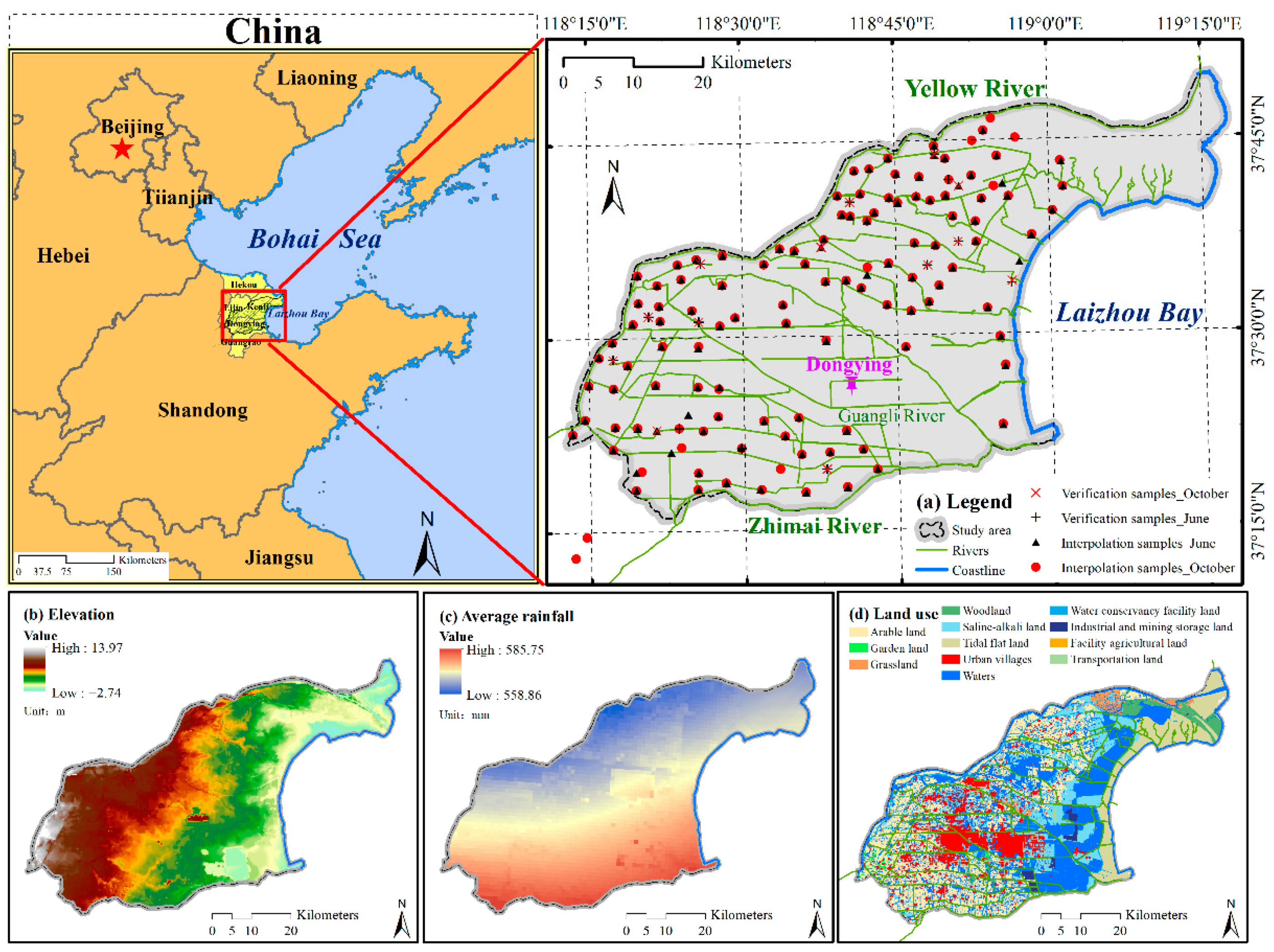
Figure 1. Study region.
Sustainability 14 06078 g001
Figure 2. Auxiliary geographic data of (a) Sand, (b) Silt, (c) Clay, (d) Slope, (e) Flow, (f) DS, (g) Average NDVI, (h) Population, and (i) GDP.
Sustainability 14 06078 g002
Figure 3. Distributions of the concentrations of STN in June, October, and SOM in June.
Sustainability 14 06078 g003
Figure 4. Correlation analysis between spatial STN changes (left) and soil erodibility (K) (right).
Sustainability 14 06078 g004
Figure 5. Correlation analysis between spatial STN status and soil erodibility (K), and soil loss in different land uses. (Notes: (a) Mean STN concentrations of different land uses in June, (b) Mean STN concentrations of different land uses in October, (c) Mean STN changes of different land uses, (d) Summary STN changes of different land uses, (e) Correlation between summary STN changes and summary K value in different land uses, and (f) Correlation between summary STN changes and summary SNLRIs in different land uses.).
Sustainability 14 06078 g005
Figure 6. Spatial distribution of soil loss risks of the influence factors in SNLRI.
Sustainability 14 06078 g006
Figure 7. Spatial distributions of (a) SNCI, (b) SNLRI, (c) A-SNNRI, and (d) A-SNNRI statistics.
Sustainability 14 06078 g007
Table 1. Correlations between soil indicators and environmental factors.
Pearson Correlations (SPSS)ElevationDSSandSiltClayNDVIRainfallPopulationq Statistic (Geodetector)Land Use
STN_June a0.0850.1740.111−0.103−0.1080.322 **0.0480.254 **STN_June d0.392 **
STN_October b0.205 *0.316 **0.020−0.017−0.0160.343 **0.1480.230 *STN_October d0.377 **
SOM_June c0.1010.200 *0.135−0.126−0.1320.336 **0.0530.257 **SOM_June d0.370 **
STN change d0.362 **0.655 **0.184 **−0.190 **−0.173 **0.118 *0.456**0.413 **STN change d0.127 **
**. Correlation is significant at the 0.01 level (2-tailed). *. Correlation is significant at the 0.05 level (2-tailed). a. Listwise N = 113; b. Listwise N = 114; c. Listwise N = 113; d. Listwise N = 281.
Table 2. Correlations between A-SNNRIs and population, GDP, and DS.
Pearson Correlations cA-SNNRIPopulationGDPDS
A-SNNRI10.164 *0.280 **−0.298 **
Population 10.785 **0.252 **
GDP 10.254 **
DS 1
*. Correlation is significant at the 0.05 level (2-tailed). **. Correlation is significant at the 0.01 level (2-tailed). c. Listwise N = 168.
Publisher’s Note: MDPI stays neutral with regard to jurisdictional claims in published maps and institutional affiliations.