
A Location Inventory Routing Optimisation Model and Algorithm for a Remote Island Shipping Network considering Emergency Inventory

Abstract
:1. Introduction
2. Mathematical Model
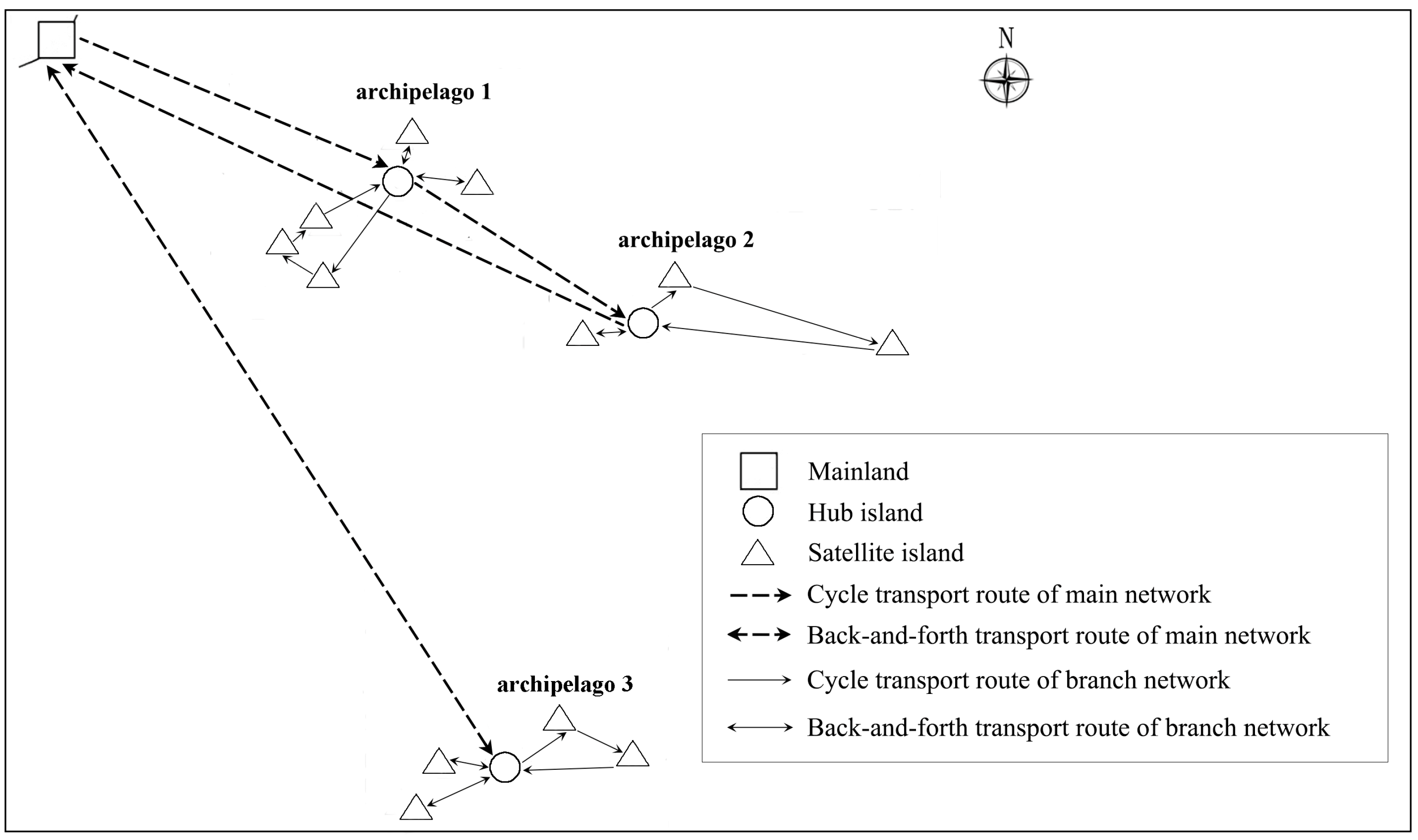
2.1. Problem Description
2.2. Notations
2.3. Model Formulation
2.3.1. Shipping Cost Model
2.3.2. Wharf Construction Cost Model
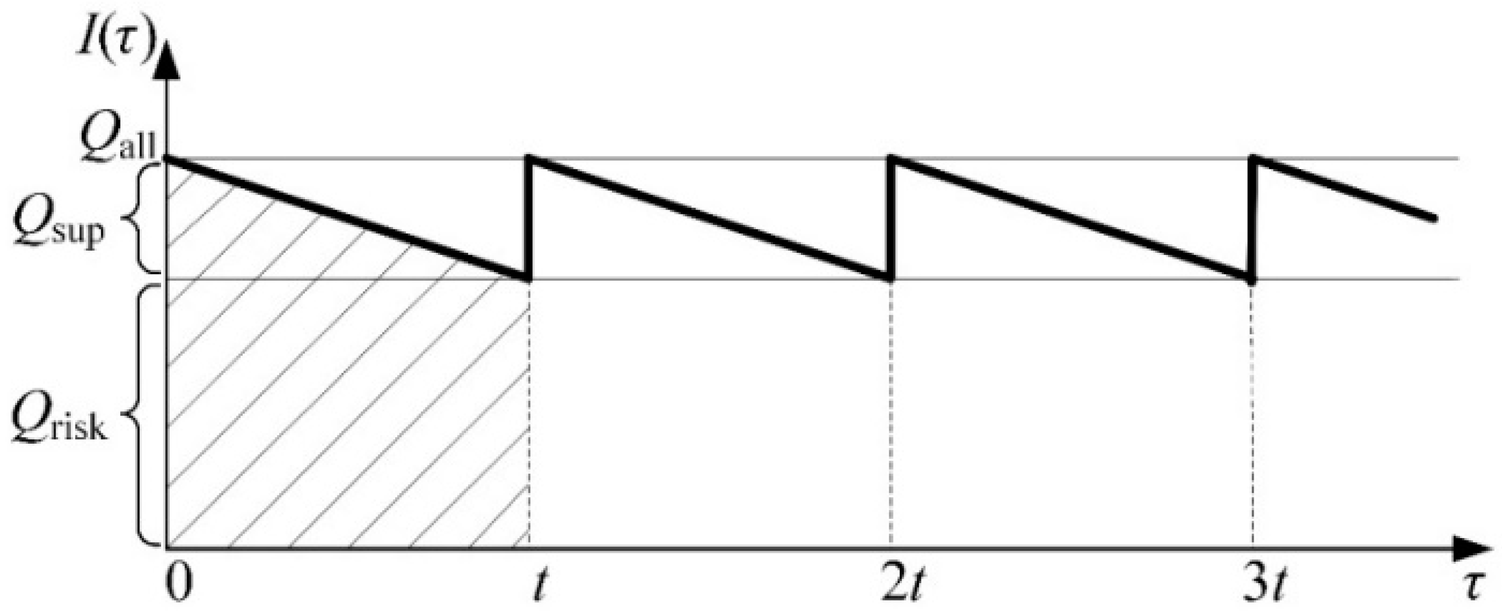
2.3.3. Inventory Cost Model
2.3.4. Formulation
3. Algorithm
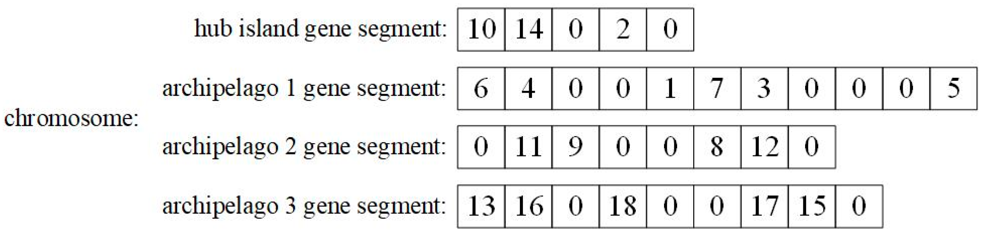
3.1. Chromosome Representation
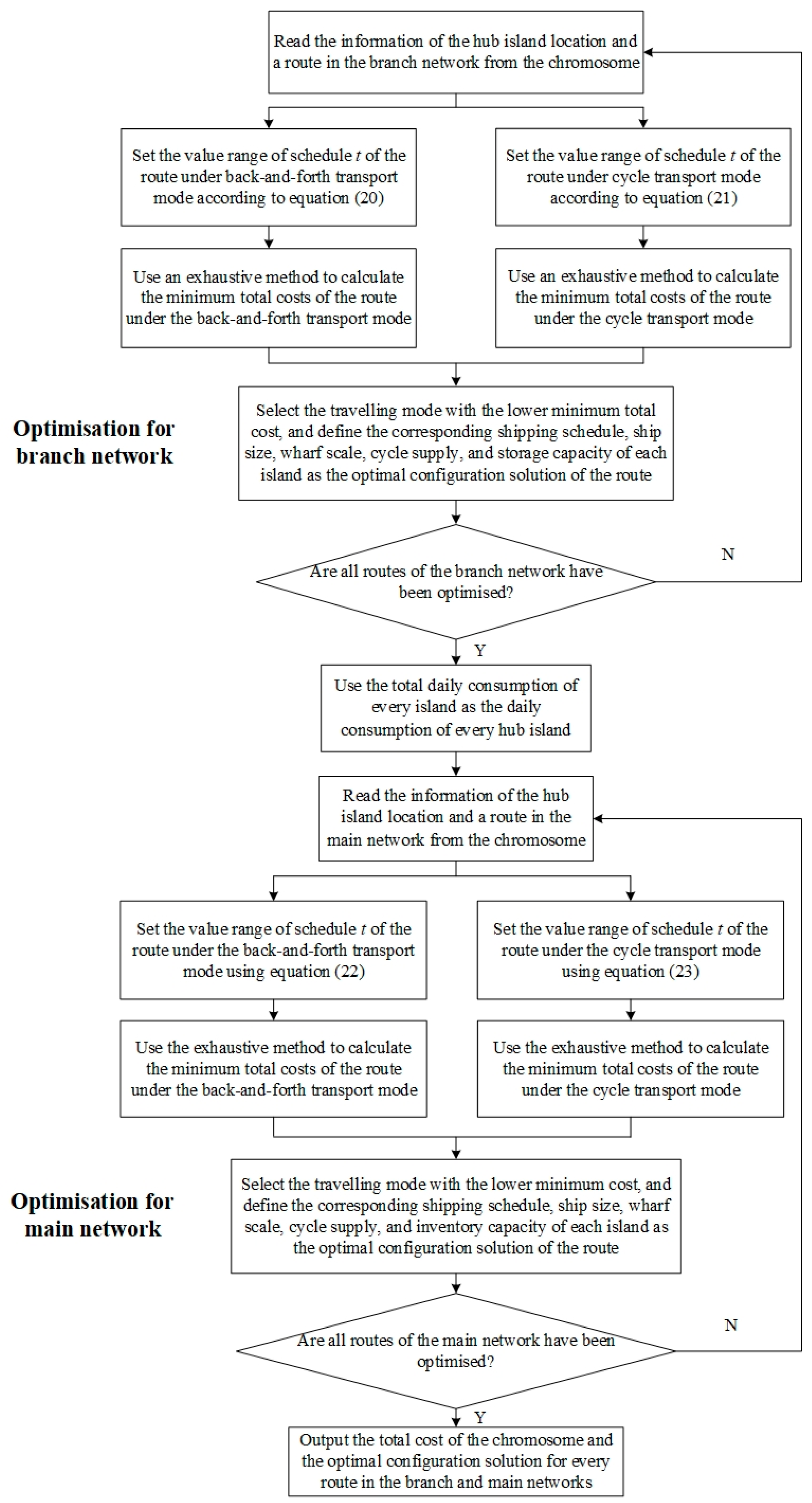
3.2. SC Module
- Step 1.
- Decode the information of the hub island location and a route in the branch network from the chromosome.
- Step 2.
- Set the value range of schedule of the route under back-and-forth and cycle transport modes according to Equations (20) and (21).
- Step 3.
- Use an exhaustive method, with as an independent variable, to calculate the minimum total costs of the route under the back-and-forth and cycle transport modes.
- Step 4.
- Select the travelling mode with the lower minimum total cost, and define the corresponding shipping schedule, ship size, wharf scale, cycle supply, and inventory capacity of each island as the optimal configuration solution for the route.
- Step 5.
- Repeat steps 1 to 4 and configure all routes in the branch network.
- Step 6.
- Use the total daily consumption of every island as the daily consumption of every hub island.
- Step 7.
- Decode the information of the hub island location and a route in the main network from the chromosome.
- Step 8.
- Set the value range of schedule of the route under the back-and-forth transport and cycle transport modes using Equations (22) and (23).
- Step 9.
- Use the exhaustive method, with as the independent variable, to calculate the minimum total costs of the route under the back-and-forth and cycle transport modes.
- Step 10.
- Select the travelling mode with the lower minimum cost, and define the corresponding shipping schedule, ship size, wharf scale, cycle supply, and inventory capacity of each island as the optimal configuration solution for the route.
- Step 11.
- Repeat steps 7 to 10 and configure all routes in the main network.
- Step 12.
- Output the total cost of the chromosome and the optimal configuration solution for every route in the branch and main networks.
3.3. Fitness
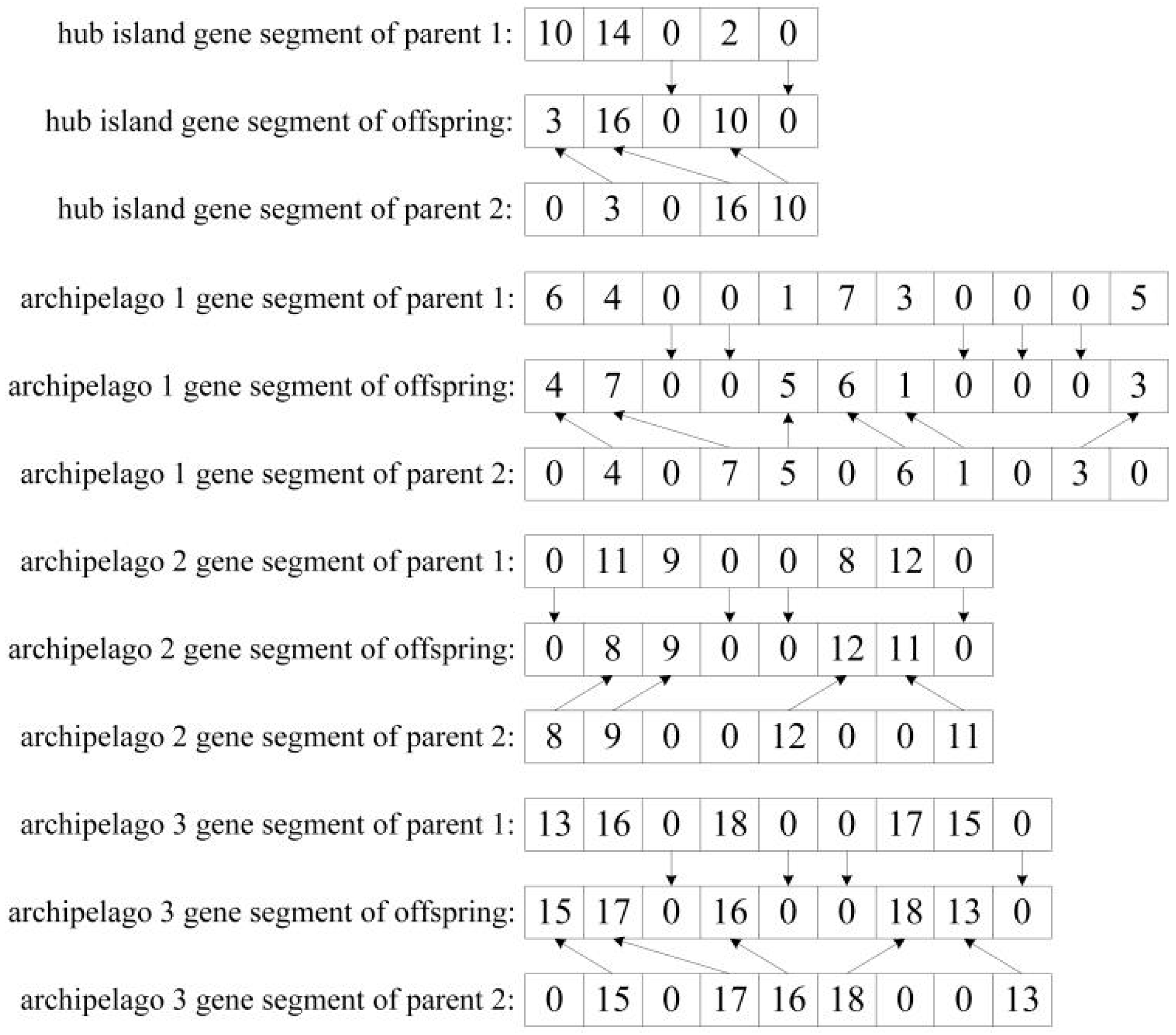
3.4. Crossover
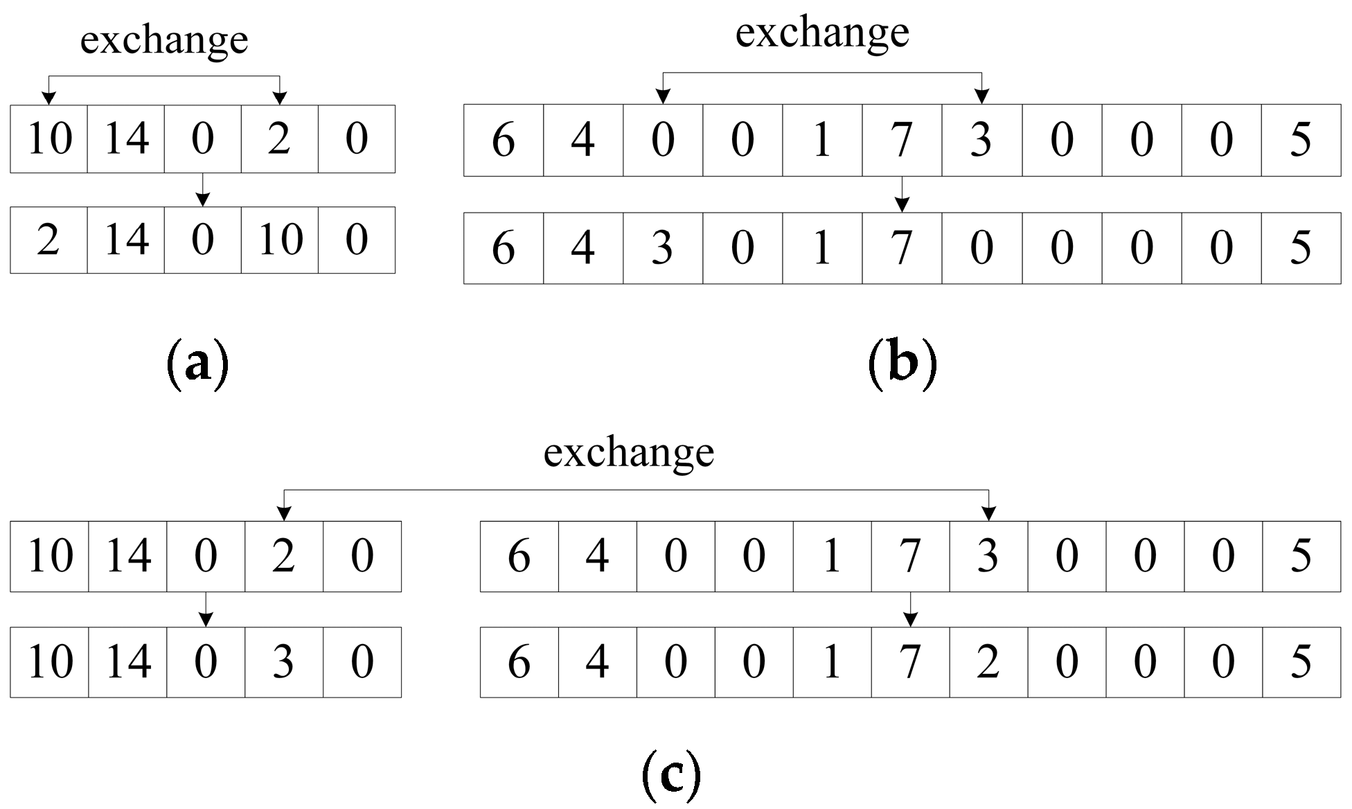
3.5. Mutation
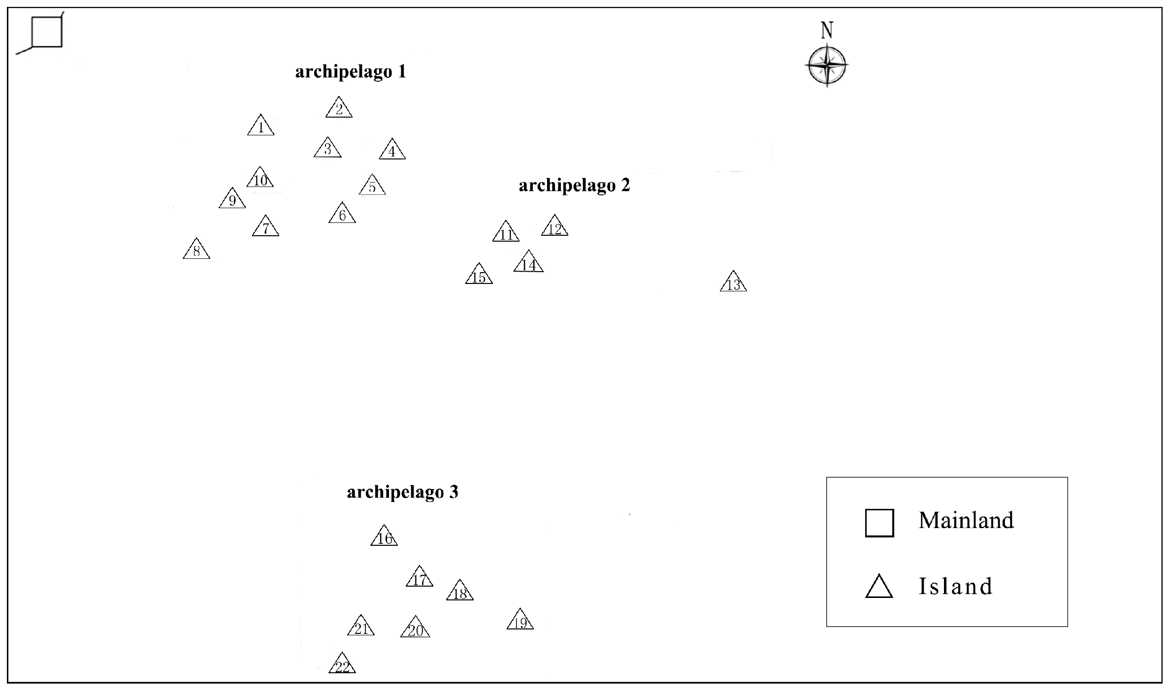
4. Instance Calculation
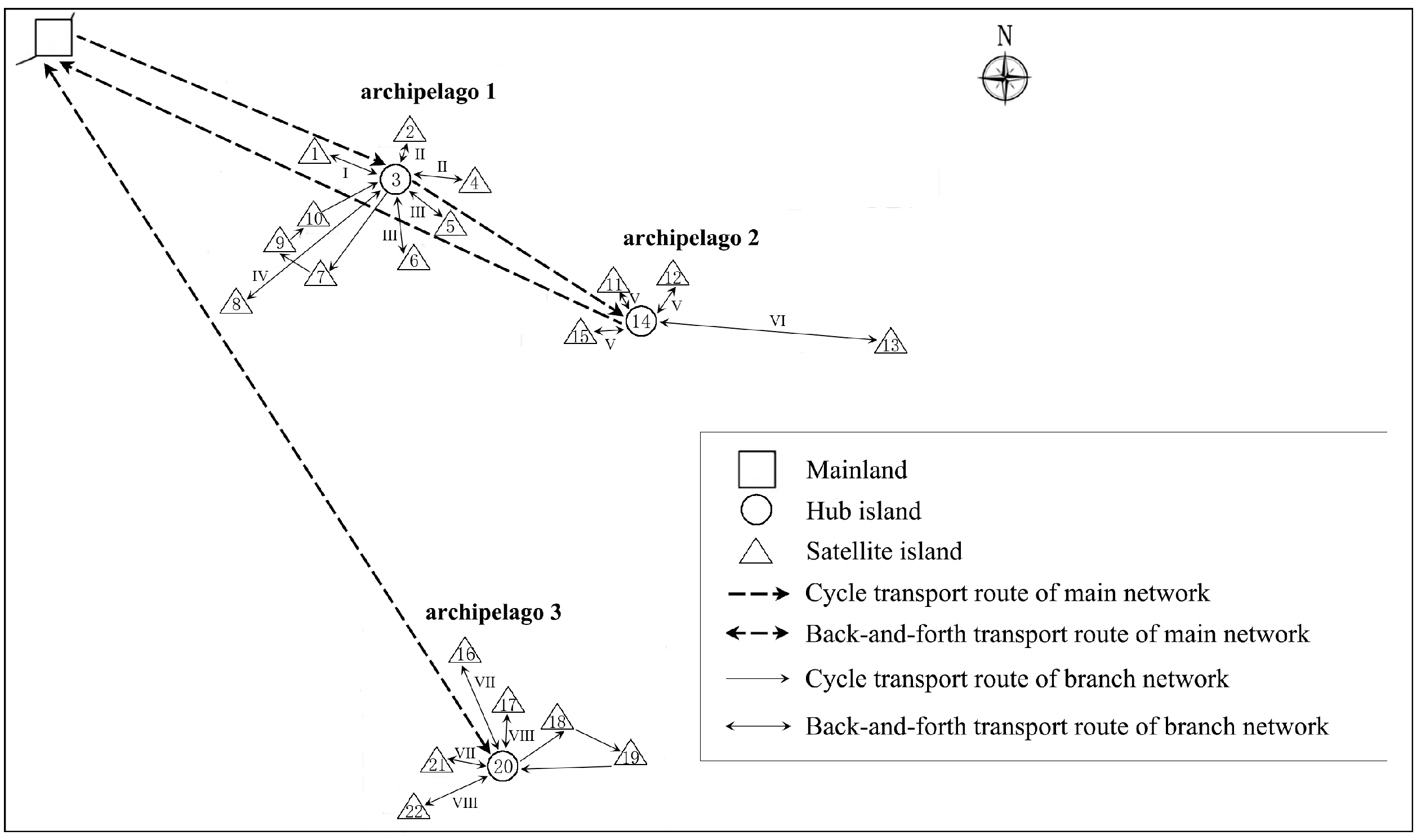
4.1. Basic Instance and Its Results
4.1.1. Data for the Basic Instance
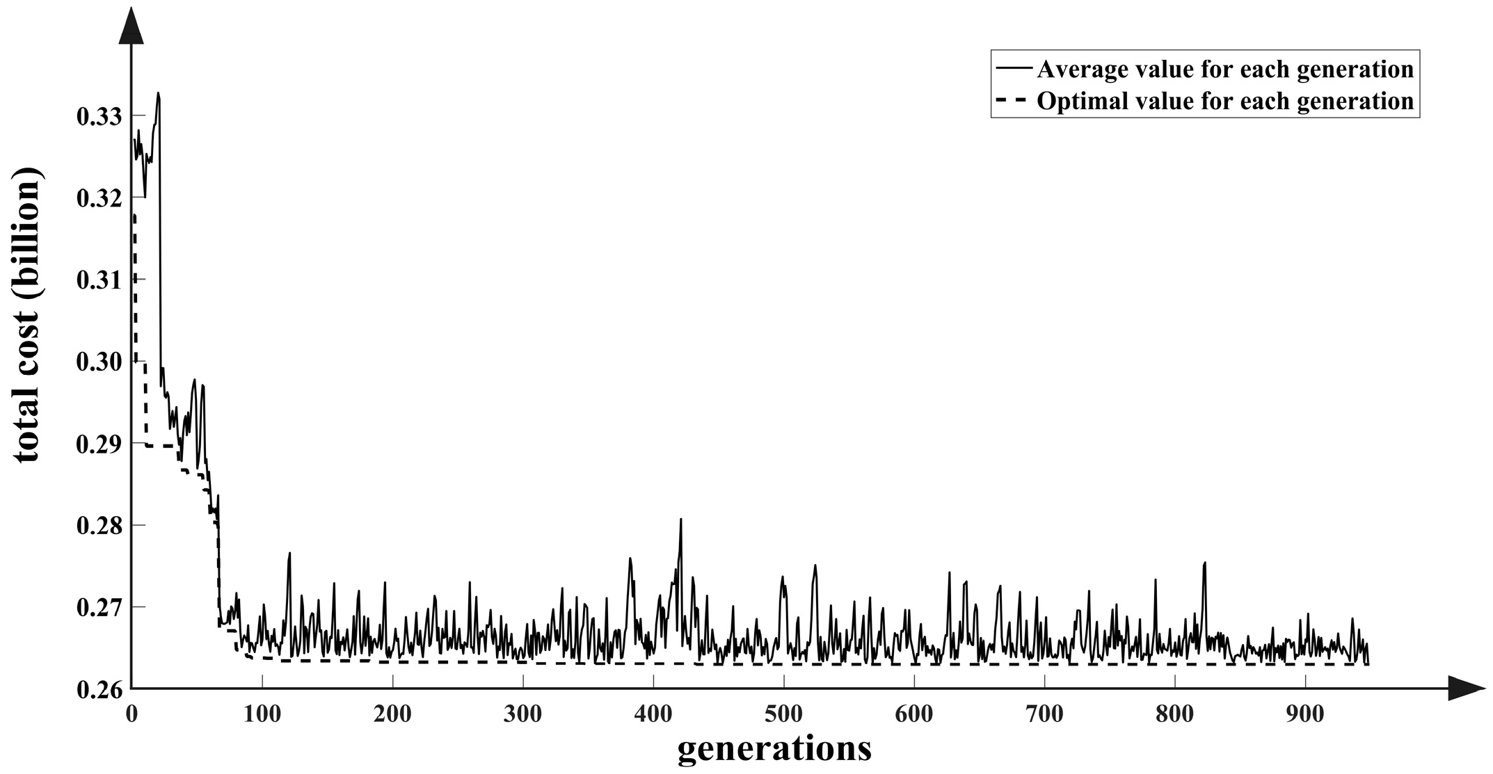
4.1.2. Results of the Basic Algorithm
4.2. Different Sizes of Instances and Their Results
4.2.1. Instance of Different Number of Islands
4.2.2. Instance of Different Demand Levels
4.3. Algorithm Comparison
5. Conclusions
6. Lessons to Be Learnt
Author Contributions
Funding
Institutional Review Board Statement
Informed Consent Statement
Data Availability Statement
Acknowledgments
Conflicts of Interest
References
- Christiansen, M.; Hellsten, E.; Pisinger, D.; Sacramento, D.; Vilhelmsen, C. Liner shipping network design. Eur. J. Oper. Res. 2020, 286, 1–20. [Google Scholar] [CrossRef]
- Brouer, B.D.; Karsten, C.V.; Pisinger, D. Optimization in liner shipping. Ann. Oper. Res. 2018, 271, 205–236. [Google Scholar] [CrossRef] [Green Version]
- Santini, A.; Plum, C.E.M.; Ropke, S. A branch-and-price approach to the feeder network design problem. Eur. J. Oper. Res. 2018, 264, 607–622. [Google Scholar] [CrossRef] [Green Version]
- Cariou, P.; Cheaitou, A.; Larbi, R.; Hamdan, S. Liner shipping network design with emission control areas: A genetic algorithm-based approach. Transp. Res. D Transp. Environ. 2018, 63, 604–621. [Google Scholar] [CrossRef]
- Wang, Y.; Meng, Q.; Kuang, H. Intercontinental Liner Shipping Service Des. Transp. Sci. 2019, 53, 344–364. [Google Scholar] [CrossRef]
- Zhen, L.; Wu, Y.; Wang, S.; Laporte, G. Green technology adoption for fleet deployment in a shipping network. Transp. Res. Part B Methodol. 2020, 139, 388–410. [Google Scholar] [CrossRef]
- Wang, S.; Dan, Z.; Lu, Z.; Lee, C. Liner Shipping Service Planning Under Sulfur Emission Regulations. Transp. Sci. 2021, 55, 491–509. [Google Scholar] [CrossRef]
- Da Costa Fontes, F.F.; Goncalves, G. A new hub network design integrating deep sea and short sea services at liner shipping operations. Int. J. Shipp. Transp. Logist. 2017, 9, 580–600. [Google Scholar] [CrossRef]
- Rahmawan, A.K.; Angelina, N. Indonesian Maritime Logistics Network Optimization Using Mixed Integer Programming. In Proceedings of the 2017 International Conference on Mechanical, Aeronautical and Automotive Engineering, Malacca, Malaysia, 25–27 February 2017. [Google Scholar]
- Papageorgiou, D.J.; Nemhauser, G.L.; Sokol, J.; Cheon, M.; Keha, A.B. MIRPLib–A library of maritime inventory routing problem instances: Survey, core model, and benchmark results. Eur. J. Oper. Res. 2014, 235, 350–366. [Google Scholar] [CrossRef]
- Agra, A.; Andersson, H.; Christiansen, M.; Wolsey, L. A Maritime Inventory Routing Problem: Discrete Time Formulations and Valid Inequalities. Networks 2013, 62, 297–314. [Google Scholar] [CrossRef] [Green Version]
- Friske, M.W.; Buriol, L.S. Applying a Relax-and-Fix Approach to a Fixed Charge Network Flow Model of a Maritime Inventory Routing Problem. In Proceedings of the 9th International Conference on Computational Logistics, Vietri sul Mare, Italy, 1–3 October 2018. [Google Scholar]
- Papageorgiou, D.J.; Cheon, M.; Nemhauser, G.; Sokol, J. Approximate Dynamic Programming for a Class of Long-Horizon Maritime Inventory Routing Problems. Transp. Sci. 2015, 49, 870–885. [Google Scholar] [CrossRef] [Green Version]
- Rodrigues, F.; Agra, A.; Christiansen, M.; Hvattum, L.M.; Requejo, C. Comparing techniques for modelling uncertainty in a maritime inventory routing problem. Eur. J. Oper. Res. 2019, 277, 831–845. [Google Scholar] [CrossRef]
- Agra, A.; Christiansen, M.; Delgado, A.; Hvattum, L.M. A maritime inventory routing problem with stochastic sailing and port times. Comput. Oper. Res. 2015, 61, 18–30. [Google Scholar] [CrossRef] [Green Version]
- Rusdianto, M.; Siswanto, N.; Iop, P. Maritime inventory routing problem with undedicated compartments: A case study from the cement industry. In Proceedings of the 2nd International Conference on Industrial and Manufacturing Engineering, Medan, Indonesia, 3–4 September 2020; Universitas Sumatera Utara, Industrial Engineering Department: Medan, Indonesia, 2020. [Google Scholar]
- Dauzere-Peres, S.; Nordli, A.; Olstad, A.; Haugen, K.; Koester, U.; Myrstad, P.O.; Teistklub, G.; Reistad, A. Omya Hustadmarmor optimizes its supply chain for delivering calcium carbonate slurry to European paper manufacturers. Interfaces 2007, 37, 39–51. [Google Scholar] [CrossRef]
- Christiansen, M.; Fagerholt, K.; Flatberg, T.; Haugen, O.; Kloster, O.; Lund, E.H. Maritime inventory routing with multiple products: A case study from the cement industry. Eur. J. Oper. Res. 2011, 208, 86–94. [Google Scholar] [CrossRef]
- Yang, A.; Wang, R.M.; Sun, Y.H.; Chen, K.; Chen, Z.G. Coastal Shuttle Tanker Scheduling Model Considering Inventory Cost and System Reliability. IEEE Access 2020, 8, 193935–193954. [Google Scholar] [CrossRef]
- Moin, N.H.; Salhi, S.; Aziz, N.A.B. An efficient hybrid genetic algorithm for the multi-product multi-period inventory routing problem. Int. J. Prod. Econ. 2011, 133, 334–343. [Google Scholar] [CrossRef]
- Papageorgiou, D.J.; Cheon, M.; Harwood, S.; Trespalacios, F.; Nemhauser, G.L. Recent progress using matheuristics for strategic maritime inventory routing. In Modeling, Computing and Data Handling Methodologies for Maritime Transportation; Konstantopoulos, C., Pantziou, G., Eds.; Springer: Cham, Switzerland, 2018; pp. 59–94. [Google Scholar]
- Friske, M.W.; Buriol, L.S.; Camponogara, E. A relax-and-fix and fix-and-optimize algorithm for a Maritime Inventory Routing Problem. Comput. Oper. Res. 2022, 137, 105520. [Google Scholar] [CrossRef]
- Eide, L.; Ardal, G.; Evsikova, N.; Hvattum, L.M.; Urrutia, S. Load-dependent speed optimization in maritime inventory routing. Comput. Oper. Res. 2020, 123, 105051. [Google Scholar] [CrossRef]
- Liu, B.T.; Zhang, Q.; Yuan, Z.H. Two-stage distributionally robust optimization for maritime inventory routing. Comput. Chem. Eng. 2021, 149, 107307. [Google Scholar] [CrossRef]
- Sanghikian, N.; Martinelli, R.; Abu-Marrul, V. A hybrid VNS for the multi-product maritime inventory routing problem. In Proceedings of the International Conference on Variable Neighborhood Search, Abu Dhabi, United Arab Emirates, 21–25 March 2021. [Google Scholar]
- Misra, S.; Kapadi, M.; Gudi, R.D. A multi grid discrete time based framework for maritime distribution logistics & inventory planning for refinery products. Comput. Ind. Eng. 2020, 146, 106568. [Google Scholar] [CrossRef]
- Engineer, F.G.; Furman, K.C.; Nemhauser, G.L.; Savelsbergh, M.W.P.; Song, J. A Branch-Price-and-Cut Algorithm for Single-Product Maritime Inventory Routing. Oper. Res. 2012, 60, 106–122. [Google Scholar] [CrossRef]
- Hewitt, M.; Nemhauser, G.; Savelsbergh, M.; Song, J. A branch-and-price guided search approach to maritime inventory routing. Comput. Oper. Res. 2013, 40, 1410–1419. [Google Scholar] [CrossRef]
- Rakke, J.G.; Andersson, H.; Christiansen, M.; Desaulniers, G. A New Formulation Based on Customer Delivery Patterns for a Maritime Inventory Routing Problem. Transp. Sci. 2015, 49, 384–401. [Google Scholar] [CrossRef]
- Song, J.; Furman, K.C. A maritime inventory routing problem: Practical approach. Comput. Oper. Res. 2013, 40, 657–665. [Google Scholar] [CrossRef]
- Hiassat, A.; Diabat, A.; Rahwan, I. A genetic algorithm approach for location-inventory-routing problem with perishable products. J. Manuf. Syst. 2017, 42, 93–103. [Google Scholar] [CrossRef]
- Saif-Eddine, A.S.; El-Beheiry, M.M.; El-Kharbotly, A.K. An improved genetic algorithm for optimizing total supply chain cost in inventory location routing problem. Ain Shams Eng. J. 2019, 10, 63–76. [Google Scholar] [CrossRef]
- Kechmane, L.; Nsiri, B.; Baalal, A. Optimization of a Two-Echelon Location Lot-Sizing Routing Problem with Deterministic Demand. Math. Probl. Eng. 2018, 2018, 2745437. [Google Scholar] [CrossRef]
- Kaya, O.; Ozkok, D. A Blood Bank Network Design Problem with Integrated Facility Location, Inventory and Routing Decisions. Netw. Spat. Econ. 2020, 20, 757–783. [Google Scholar] [CrossRef]
- Saragih, N.I.; Bahagia, S.N.; Suprayogi; Syabri, I. A heuristic method for location-inventory-routing problem in a three-echelon supply chain system. Comput. Ind. Eng. 2019, 127, 875–886. [Google Scholar] [CrossRef]
- Guo, H.; Li, C.D.; Zhang, Y.; Zhang, C.N.; Wang, Y. A Nonlinear Integer Programming Model for Integrated Location, Inventory, and Routing Decisions in a Closed-Loop Supply Chain. Complexity 2018, 2018, 2726070. [Google Scholar] [CrossRef]
- Liu, B.L.; Chen, H.; Li, Y.H.; Liu, X. A Pseudo-Parallel Genetic Algorithm Integrating Simulated Annealing for Stochastic Location-Inventory-Routing Problem with Consideration of Returns in E-Commerce. Discret. Dyn. Nat. Soc. 2015, 2015, 586581. [Google Scholar] [CrossRef]
- Zhu, Q.; Krikke, H. Managing a Sustainable and Resilient Perishable Food Supply Chain (PFSC) after an Outbreak. Sustainability 2020, 12, 5004. [Google Scholar] [CrossRef]
- Lee, A.; Kang, H.Y.; Ye, S.J.; Wu, W.Y. An Integrated Approach for Sustainable Supply Chain Management with Replenishment, Transportation, and Production Decisions. Sustainability 2018, 10, 3887. [Google Scholar] [CrossRef] [Green Version]
- Kungwalsong, K.; Cheng, C.Y.; Yuangyai, C.; Janjarassuk, U. Two-Stage Stochastic Program for Supply Chain Network Design under Facility Disruptions. Sustainability 2021, 13, 2596. [Google Scholar] [CrossRef]
- Lin, Y.S.; Wang, X.F.; Hu, H.; Zhao, H. Research on feeder network design: A case study of feeder service for the port of Kotka. Eur. Transp. Res. Rev. 2020, 12, 61. [Google Scholar] [CrossRef]
- Qin, J.; Ye, Y.; Cheng, B.R.; Zhao, X.B.; Ni, L.L. The Emergency Vehicle Routing Problem with Uncertain Demand under Sustainability Environments. Sustainability 2017, 9, 288. [Google Scholar] [CrossRef] [Green Version]

| Literature | Location | Inventory | Routing | Emergency Inventory | Multi-Size Carrier | Multi-Travelling Mode | Transport Schedule |
|---|---|---|---|---|---|---|---|
| Papageorgiou et al. (2014) [10] Agra et al. (2013) [11] Friske and Buriol (2018) [12] Papageorgiou et al. (2015) [13] Rusdianto et al. (2020) [16] Yang et al. (2020) [19] Hewitt et al. (2013) [28] Song and Furman (2013) [30] Friske et al. (2022) [22] Sanghikian et al. (2021) [25] Eide et al. (2020) [23] Liu et al. (2021) [24] | √ | √ | √ | √ | |||
| Rodrigues et al. (2019) [14] Dauzere-Peres et al. (2007) [17] Christiansen et al. (2011) [18] Engineer et al. (2012) [27] | √ | √ | √ | √ | √ | ||
| Agra et al. (2015) [15] Papageorgiou et al. (2018) [21] | √ | √ | √ | √ | √ | ||
| Moin et al. (2011) [20] | √ | √ | √ | ||||
| Rakke et al. (2015) [29] | √ | √ | √ | √ | |||
| Misra et al. (2020) [26] | √ | √ | √ | √ | √ | ||
| Hiassat et al. (2017) [31] Kechmane et al. (2018) [33] Kaya and Ozkok (2020) [34] | √ | √ | √ | √ | |||
| Saif-Eddine et al. (2019) [32] | √ | √ | √ | √ | √ | ||
| Saragih et al. (2019) [35] | √ | √ | √ | √ | √ | ||
| Guo et al. (2018) [36] Liu et al. (2015) [37] | √ | √ | √ | √ | √ | ||
| This paper | √ | √ | √ | √ | √ | √ | √ |
| Acronyms | |
|---|---|
| Back-and-forth routing group | |
| Cycle routing | |
| Inventory | |
| Warehouse construction | |
| Sets | |
| . | |
| Parameters | |
| The mainland port | |
| The number of the archipelago | |
| . | |
| The total shipping costs of the BFRG and the CR in the branch network, respectively | |
| The total shipping costs of the BFRG and CR in the main network, respectively MBFRG means the back-and-forth routing group in the main network; MCR means the cycle routing in the main network | |
| The ship usage cost | |
| The wharf construction cost | |
| The inventory cost and warehouse construction cost, respectively | |
| Sailing speed of a ship | |
| The total time of system operation (days) | |
| Discrete decision variables | |
| , e.g., if island 3# is the hub island of archipelago , then = 3#. | |
| in the branch network, e.g., if the CR 3 in the branch network is 2#→3#→7#→1#→. | |
| in the main network. | |
| in the branch network, e.g., if CR 3 in the branch network is 2#→3#→7#→1#→2#, then | |
| →2#→15#→22#→. | |
| Continuous decision variables | |
| in the branch network, respectively | |
| in the main network, respectively | |
| Any moment in a transport schedule | |
| Binary decision variables | |
| Island | Daily Supply Demand (tons) | Island | Daily Supply Demand (tons) | Island | Daily Supply Demand (tons) |
|---|---|---|---|---|---|
| 1# | 21 | 9# | 40 | 17# | 120 |
| 2# | 31 | 10# | 59 | 18# | 73 |
| 3# | 191 | 11# | 25 | 19# | 61 |
| 4# | 33 | 12# | 10 | 20# | 181 |
| 5# | 132 | 13# | 31 | 21# | 80 |
| 6# | 119 | 14# | 40 | 22# | 104 |
| 7# | 52 | 15# | 12 | ||
| 8# | 171 | 16# | 96 |
| Ship Size (Tonnage Class) | Purchase Costs (Thousand Dollars) | Daily Maintenance Costs (Thousand Dollars/Month) | Shipping Costs (Dollar/Nautical Mile) | Corresponding Wharf Construction Costs (Thousand Dollars) |
|---|---|---|---|---|
| 100 | 40 | 0.68 | 0.8 | 2000 |
| 500 | 150 | 1.40 | 2.5 | 6000 |
| 1000 | 280 | 1.88 | 3.0 | 10,000 |
| 5000 | 1200 | 4.00 | 7.0 | 20,000 |
| 10,000 | 1800 | 4.80 | 8.5 | 24,000 |
| 15,000 | 2500 | 6.00 | 10.0 | 30,000 |
| 20,000 | 3000 | 6.50 | 12.0 | 32,000 |
| Route | The Cycle Route from the Mainland to Hub Island | The Back-and-Forth Route from the Mainland to Hub Island |
|---|---|---|
| Islands and order of visit | 3#, 14# | 20# |
| Ship size (tonnage class) | 5000 | 5000 |
| Schedule (days) | 5 | 6 |
| Route | Cycle Route I | Back-and-Forth Route Group I | Back-and-Forth Route Group II | Back-and-Forth Route Group III | Back-and-Forth Route Group IV |
|---|---|---|---|---|---|
| Islands and order of visit | 7#, 9#, 10# | 1# | 2#, 4# | 5#, 6# | 8# |
| Ship size (tonnage class) | 500 | 100 | 100 | 500 | 1000 |
| Schedule (days) | 3 | 4 | 3 | 3 | 4 |
| Route | Back-and-Forth Route Group V | Back-and-Forth Route Group VI |
|---|---|---|
| Islands and order of visit | 11#, 12#, 15# | 13# |
| Ship size (tonnage class) | 100 | 100 |
| Schedule (days) | 4 | 3 |
| Route | Cycle Route II | Back-and-Forth Route Group VII | Back-and-Forth Route Group VIII |
|---|---|---|---|
| Islands and order of visit | 18#, 19# | 16#, 21# | 17#, 22# |
| Ship size (tonnage class) | 500 | 500 | 500 |
| Schedule (days) | 3 | 5 | 4 |
| Archipelago | Island | Number (Berth) | Berth (Tonnage Class) | Inventory Capacity (Tons) | Supply (Tons) |
|---|---|---|---|---|---|
| Archipelago 1 | 1# | 1 | 100 | 189 | 84 |
| 2# | 1 | 100 | 248 | 93 | |
| 3# | 4 | 100, 500, 1000, 5000 | 8490 | 4245 | |
| 4# | 1 | 100 | 264 | 99 | |
| 5# | 1 | 500 | 1056 | 396 | |
| 6# | 1 | 500 | 952 | 357 | |
| 7# | 1 | 500 | 416 | 156 | |
| 8# | 1 | 1000 | 1539 | 684 | |
| 9# | 1 | 500 | 320 | 120 | |
| 10# | 1 | 500 | 472 | 177 | |
| Archipelago 2 | 11# | 1 | 100 | 225 | 100 |
| 12# | 1 | 100 | 90 | 40 | |
| 13# | 1 | 100 | 248 | 93 | |
| 14# | 2 | 100, 5000 | 1180 | 590 | |
| 15# | 1 | 100 | 108 | 48 | |
| Archipelago 3 | 16# | 1 | 500 | 960 | 480 |
| 17# | 1 | 500 | 1080 | 480 | |
| 18# | 1 | 500 | 584 | 219 | |
| 19# | 1 | 500 | 488 | 183 | |
| 20# | 2 | 500, 5000 | 7865 | 4290 | |
| 21# | 1 | 500 | 800 | 400 | |
| 22# | 1 | 500 | 936 | 416 |
| Number of Islands | Calculation Results (Thousand Dollars) | Number of Occurrences of the Best Optimisation Result | Average Calculation Time (s) | ||
|---|---|---|---|---|---|
| Best Optimisation Result | Average Value | Standard Deviation | |||
| 22 (basic instance) | 262,949.40 | 266,796.34 | 4681.11 | 5 | 330.84 |
| 28 | 338,808.57 | 338,973.90 | 252.75 | 7 | 548.73 |
| 34 | 403,613.77 | 403,633.46 | 52.29 | 8 | 905.27 |
| 40 | 469,668.34 | 471,765.72 | 2097.40 | 5 | 1113.26 |
| Demand Levels | Calculation Results (Thousand Dollars) | Number of Occurrences of the Best Optimisation Result | Average Calculation Time (s) | ||
|---|---|---|---|---|---|
| Best Optimisation Result | Average Value | Standard Deviation | |||
| 100% (basic instance) | 262,949.40 | 266,796.34 | 4681.11 | 5 | 330.84 |
| 120% | 299,987.96 | 299,988.06 | 0.30 | 9 | 501.37 |
| 140% | 340,076.01 | 340,076.01 | 0.00 | 10 | 373.33 |
| 160% | 357,156.68 | 357,362.02 | 407.12 | 7 | 455.61 |
| Algorithm | Optimisation Results | Calculation Time | ||||
|---|---|---|---|---|---|---|
| Best Optimisation Result (Thousand Dollars) | Difference from SC-GA (%) | Average Value (Thousand Dollars) | Difference from SC-GA (%) | Average Calculation Time (s) | Difference from SC-GA (%) | |
| SC-GA | 262,949.40 | - | 266,796.34 | - | 330.84 | - |
| IGA [32] | 295,381.62 | 12.33 | 310,176.77 | 16.26 | 659.72 | 99.41 |
| SA [34] | 309,389.88 | 17.66 | 317,367.36 | 18.95 | 282.34 | −14.66 |
| PPGASA [37] | 292,628.33 | 11.29 | 300,432.48 | 12.61 | 380.41 | 14.98 |
Publisher’s Note: MDPI stays neutral with regard to jurisdictional claims in published maps and institutional affiliations. |
© 2022 by the authors. Licensee MDPI, Basel, Switzerland. This article is an open access article distributed under the terms and conditions of the Creative Commons Attribution (CC BY) license (https://creativecommons.org/licenses/by/4.0/).
Share and Cite
Wu, D.; Ji, X.; Xiao, F.; Sheng, S. A Location Inventory Routing Optimisation Model and Algorithm for a Remote Island Shipping Network considering Emergency Inventory. Sustainability 2022, 14, 5859. https://doi.org/10.3390/su14105859
Wu D, Ji X, Xiao F, Sheng S. A Location Inventory Routing Optimisation Model and Algorithm for a Remote Island Shipping Network considering Emergency Inventory. Sustainability. 2022; 14(10):5859. https://doi.org/10.3390/su14105859
Chicago/Turabian StyleWu, Di, Xuejun Ji, Fang Xiao, and Shijie Sheng. 2022. "A Location Inventory Routing Optimisation Model and Algorithm for a Remote Island Shipping Network considering Emergency Inventory" Sustainability 14, no. 10: 5859. https://doi.org/10.3390/su14105859
APA StyleWu, D., Ji, X., Xiao, F., & Sheng, S. (2022). A Location Inventory Routing Optimisation Model and Algorithm for a Remote Island Shipping Network considering Emergency Inventory. Sustainability, 14(10), 5859. https://doi.org/10.3390/su14105859