Abstract
Estimation of the failure probability for corroded oil and gas pipelines using the appropriate reliability analysis method is a task with high importance. The accurate prediction of failure probability can contribute to the better integrity management of corroded pipelines. In this paper, the reliability analysis of corroded pipelines is investigated using different simulation and meta-model methods. This includes five simulation approaches, i.e., Monte Carlo Simulation (MCS), Directional Simulation (DS), Line Sampling (LS), Subset Simulation (SS), and Importance Sampling (IS), and two meta-models based on MCS as Kriging-MCS and Artificial Neural Network based on MCS (ANN-MCS). To implement the proposed approaches, three limit state functions (LSFs) using probabilistic burst pressure models are established. These LSFs are designed for describing the collapse failure mode for pipelines constructed of low, mid, and high strength steels and are subjected to corrosion degradation. Illustrative examples that comprise three candidate pipelines made of X52, X65, and X100 steel grade are employed. The performance and efficiency of the proposed techniques for the estimation of the failure probability are compared from different aspects, which can be a useful implementation to indicate the complexity of handling the uncertainties provided by corroded pipelines.
1. Introduction
Today’s world is dependent on energy, and one of the ways to supply energy is through fuel, especially fossil fuels [1,2]. Because of the increasing development of various industries, the necessity to transport these resources is becoming increasingly vital [3]. The transportation of oil, gas, and petrochemicals by land, sea, and air has shown that these methods of transportation, in addition to their obstacles and problems and the existence of many financial and human risks, are not economically affordable [4,5]. Transporting fossil fuel-based substances and products via pipelines is the most suitable solution as these structures are one of the safest and most cost-effective transportation ways in this industry [6]. However, pipelines are subjected to the surrounding environmental conditions that can cause irreversible consequences such as partial or full destruction if any severe degradations occur [7,8]. Despite the development advances in pipeline technology and the oil and gas industry, failure events are still witnessed [9]. Therefore, the evaluation of the pipeline safety levels is of fundamental importance.
Corrosion is among the main causes of steel pipeline failures [10], which is recognized as the most important electrochemical mechanism for imposing a cost of defect that can significantly reduce the long-term integrity of pipelines [11,12,13]. Thus, reliability-based corrosion assessment of oil and gas pipelines has become a trend in research by the scientific community and pipeline owners to handle the relevant uncertainties, such as the inherent unpredictability of corrosion growth and the measurement errors from the inline inspection tools [14,15]. Generally, reliability refers to the effective use of policies, resources, and regulations to assess and control the existing uncertainties such as in corroded pipelines [16]. Such an efficient approach is highly suggested to decrease the danger of structural collapse, which can result in fatalities, economic losses, or environmental contamination, while also allowing the designer to accomplish a cost-safety trade-off, given the current uncertainties [17]. Furthermore, local failure of pipelines can have disproportional consequences. Local loss of performance can be the root cause of loss of the entire linear component, failure (partial or complete) of the infrastructure network, and supply disruption. The performance reliability of the element can then be used as the core indicator for the assessment of the entire system’s performance in terms of redundancy [18,19] or robustness [20]. Respectively, the focus of maintenance strategies and exercises for the entire network from a life-cycle perspective should also be diverted to localized reliability assessments of individual components or sections thereof [21].
There have been several structural reliability approaches established to date, which may be split into two categories: analytical and simulation-based methods [22,23]. Analytical methods include the well-known first and second-order reliability methods (FORM and SORM), in which these approaches use the linear and quadratic approximations of the performance function to obtain the most probable point (MPP). FORM is widely considered to estimate the failure probability for different complex structural problems in engineering, including corroded pipelines [24,25]. Using the FORM method, it is necessary to convert the convex limit state functions to a line and then calculate the integral of the failure region. As a result, numerous areas in the safe region may be overlooked in this situation and incorporated into the calculation as a failure region, in which the failure probability will be over-estimated [26]. Furthermore, a considerable portion of the failure zone is deemed the safe region for functions with concave curvature, which means that the failure probability will be under-estimated. Thus, FORM may produce unstable results for non-linear problems, such as the reliability of corroded pipeline.
Simulation-based approaches, on the other hand, use random samples according to the distribution of the basic random variables to compute the system response for each variable in order to estimate the failure probability. In pipeline corrosion studies, the Monte Carlo Simulation (MCS) method, which is considered the most efficient methodology for assessing system reliability, has been utilized extensively [27,28,29,30]. The Monte Carlo approach (MCS) is based on producing a very large number of samples to cover all conceivable regions. As a result, this technique will have a high computational cost, particularly if the failure probability is low or the number of corrosion defects is enormous, as in oil and gas pipelines. To overcome the drawbacks of the MCS method, other simulation-based techniques are developed, which include importance sampling (IS) [31], line sampling (LS) [32], subset simulation (SS) [33], and directional simulation (DS) [34] methods.
Various research studies, based on different structural reliability methodologies have been undertaken so far to assess the reliability analysis of corroding pipelines. For the analytical-based methods, we cite the works of Keshtegar and Miri [35], who proposed a novel algorithm with a new sensitivity vector for reliability analysis of corroded pipelines. The new sensitivity vector was used to calculate the conjugate gradient vector of the limit state function based on the HL-RF method. Later, Mohamed EL Amine et al. [36] developed a new reliability method based on an improved FORM using the conjugate map theory and applied it to estimate the reliability index of six examples of corroded pipelines. Recently, Keshtegar et al. [37] conducted a comparative reliability analysis study of corroded pipelines based on different FORM-based methods, in which the results indicated that the original FORM method may be an unsuitable technique for handling the complexity provided by the uncertainties of corroded pipeline problems. For simulation-based methods, the Monte Carlo Simulation (MCS) is extensively utilized for solving corroded pipeline problems. Leira et al. [38] assessed the reliability analysis of corroded pipelines using an enhanced Monte Carlo Simulation method and implemented it in systems with independent and correlated corrosion defects. Gong and Zhou [31] used the importance sampling (IS) technique to investigate the time-dependent reliability of corroded pipelines in which two failure modes, small leak and burst, are considered. Novák et al. [39] demonstrated a software package for structural degradation which encompasses a series of simulation techniques, including hierarchical sampling for the establishment and the extension of the sample size, without compromising the desired correlation structure. Mohamed El Amine et al. [40] proposed a new framework for the structural reliability of APL X60 gas pipeline subjected to corrosion degradation by using a novel hybrid method that combines the MCS and machine learning model called M5 Tree model. Abyani and Bahaari [41] compared the efficiency of two simulation-based methods, including the Monte Carlo and Latin Hypercube Sampling (LHS), to conduct the reliability analysis of corroded pipelines by considering three failure modes as corrosion perforation, local burst, and rupture.
Despite the extensive advances in maintaining the safety levels of oil and gas pipelines, the structural reliability analysis is still a challenge due to the complex features provided by the uncertainties surrounding these structures. This study contributes to the structural reliability analysis of oil pipelines subjected to corrosion defects using different simulation and meta-model approaches. As previously stated, MCS is the most basic method for estimating the failure probability. The MCS, on the other hand, has a rather large computational time cost. As a result, for the failure probability estimation, an accurate approach with less computing time and more precision is required. For this objective, the accuracy and performance of four sampling-based approaches, including MCS, SS, LS, IS, and DS, as well as two meta-modeling-based methods, kriging and artificial neural network, are evaluated for the reliability analysis of corroded pipeline. The following is how the rest of the paper is organized: Section 2 describes the structural formulation of the pipeline system reliability using the limit state function concept based on the collapse failure mode; Section 3 details the proposed approaches for assessing the structural reliability analysis. In Section 4, illustrative examples are reported to appraise the effectiveness of the simulation and meta-modeling-based techniques. The acquired results are depicted and discussed in Section 5, while the conclusions and recommendations are presented in Section 6.
2. Limit State Functions of Corroded Pipelines Based on the Steel Grade
Pipelines under active corrosion defects tend to burst at an unknown stage of their residual life. Thus, accurate prediction of the failure probabilities is an important task [42,43]. Usually, the state of a corroded pipeline is modelled using a limit state function that describes the probable failure mode [44,45]. The burst failure mode due to corrosion is the most common, whereas the limit state function of a pipeline segment at the ith active corrosion defect can be formulated using Equation (1) as follows:
where X denotes a vector of input random variables, and and are the burst and operating pressures at the ith defect, respectively. Several models have been developed to model the burst pressure of corroded pipelines over the years. Keshtegar and Mohamed [46] reviewed 35 empirical models for the burst pressure in terms of the development basis, equation forms, advantages, and limitations. Furthermore, the authors compare the effectiveness of the assessed burst pressure models to a large-scale experimental test database, in which conclusions revealed that all the empirical models have a tendency to miss-estimate the real values for outside ranges of their development. Rafael Amaya-Gómez et al. [47] conducted a similar study in which several burst pressure models were examined using various criteria and the same conclusions were reached. Recently, Mohamed El Amine et al. [36] have overcome this drawback by developing new probabilistic models based on the pipelines grade as low (e.g., X46 and X52), mid (e.g., X60 and X65), and high (e.g., X80 and X100) strength steel pipelines, whereas Equations (2)–(4) give their formulas, in the same respect.
These probabilistic models consist of three terms as the model errors that are represented by for the low, medium, and high-grade pipelines, respectively. The burst pressure of intact pipes based on the average shear stress yield criterion , in which n is the strain hardening exponent while is the average diameter, D and t are the diameter and wall-thickness of the pipeline, respectively. The last term is the remaining strength factors which include the defect geometries as the depth (d) and length (L). and are dimensionless factors, where R refers to the radius of the pipeline. Thus, depending on the pipeline steel grade, three limit state functions are extracted and employed for the burst failure mode, which are provided by Equations (5)–(7) as follows [36,48]:
Unlike other limit state functions, the aforementioned ones are complex and contain several variables with different distributions and varied ranges. As a result, it is quite difficult to trust the reliability analysis results based on a single technique. Thus, the next section will detail numerous simulation and meta-model methodologies that will be used to evaluate and compare the reliability of corroded pipelines.
3. Approaches for Structural Reliability Analysis
3.1. Simulation Techniques Based on Monte Carlo Method
Generally, simulation methods estimate the failure probability by generating samples based on the random variable’s PDFs of the problem and then calculating the system response for each produced sample. Monte Carlo Simulation (MCS) is an accurate yet expensive method in terms of the necessary time for computation. Other simulation methods, including Importance Sampling (IS) [49], Subset Simulation (SS) [50], Directional Simulation (DS) [51], and Line Sampling (LS) [52], have been suggested by various researchers to compensate and overcome this weakness.
3.1.1. Monte Carlo Simulation (MCS)
The Monte Carlo Simulation (MCS) technique is the most reliable and widely used method for predicting the failure probability of complicated structural problems [53]. The design space is separated into two sections as safe and failure in this technique, based on the values of the performance function g(X). The failure zone is defined as points with g(X) < 0, while the safe zone is defined as points with g(X)> 0; the limit state function is defined as the border between these two zones, g(X) = 0. The ratio of the number of samples in the failure zone to the total samples is used to determine the failure probability as follows:
where N denotes the total number of samples and denotes the number of samples in the failure zone. I presents an indicator function of failure, which counts 1, I = 1 for samples in the failure zone and 0, I = 0 for sample in the safe zone.
3.1.2. Importance Sampling (IS)
In the important sampling (IS) approach, instead of using the probability density function with random variables, an alternate function is employed [49,54]. Thus, the production of samples occurs based on this new function and around the most important point. Therefore, the failure probability using IS is calculated as follows [31]:
where is a random variable with the PDF of .
The new PDF must meet two essential characteristics when using the IS approach. The first produces more samples in the failure region than the Monte Carlo method. The second requirement is that the new PDF function is as close to the original as feasible.
3.1.3. Subset Simulation (SS)
The subset simulation approach, which combines the Monte Carlo Simulation (MCS) and the Markov chain, allows a very accurate estimation of small failure probabilities [50,55]. The design space is partitioned into m subspaces in this procedure, and samples are created for each area separately (Figure 1). The likelihood of the failure probability in each location is then estimated. Finally, the overall failure probability is calculated by adding the probabilities of the other failure probabilities as follows [56]:
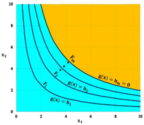
Figure 1.
Subset Simulation approach.
3.1.4. Directional Simulation (DS)
In order to use the directional simulation (DS) approach, the issue must be defined in the polar space using Equation (11) [57,58].
where is radius and A is the unit direction vector. Thus, the failure probability can be written as follows [59]:
where is the Jacobin matrix determinant, which is utilized to represent the transformation of a differential variable to a new space. represent the joint probability distribution function of A variables. is a directional simulation operator of the vector A. presents the radius length in the simulation direction of A = a (Figure 2). More details regarding this approach are available in Ref [57].
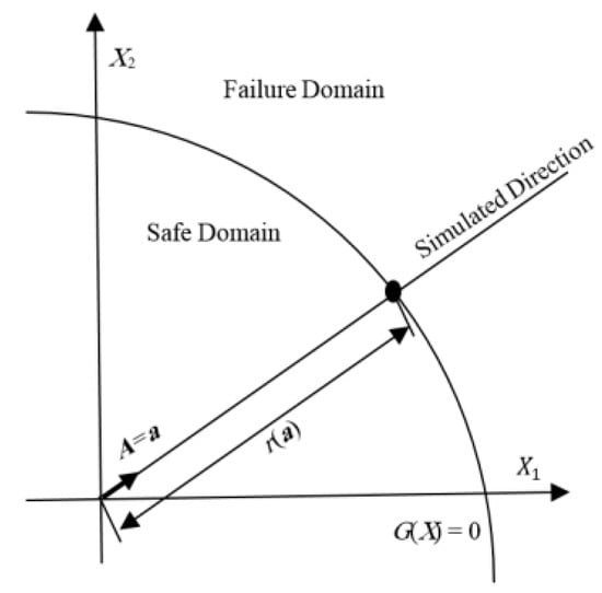
Figure 2.
Directional Simulation approach.
3.1.5. Line Sampling (LS)
The primary concept behind the line sampling (LS) strategy is to search for the failure domain in high-dimensional problems using lines rather than random samples [60,61,62]. The variables are transferred to the standard normal space as shown in Figure 3, and then the samples are generated linearly in the importance direction. In standard normal space, the importance direction connects the origin to the point with the highest risk of failure. It should be emphasized that the line sampling method’s accuracy and efficiency are dependent on the detection of importance directions.
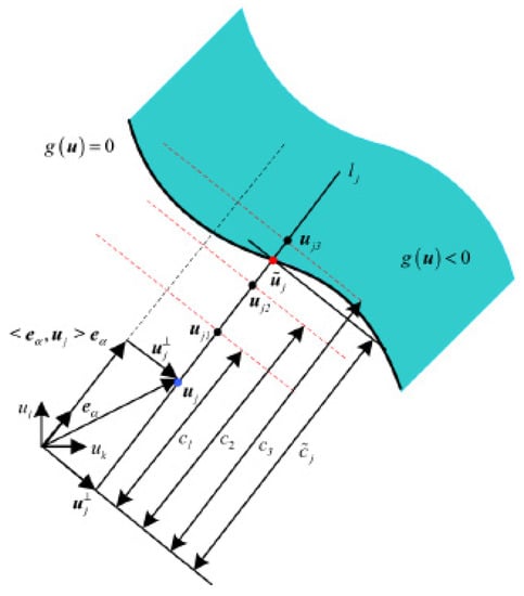
Figure 3.
Line Sampling approach.
Figure 4 depicts the entire framework for assessing the limit state functions of corroded pipelines as described in Equations (5)–(7), using simulation approaches based on MCS.
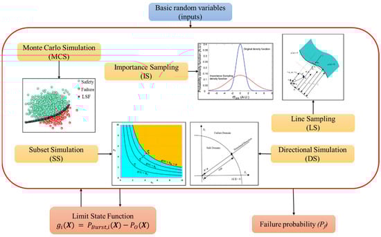
Figure 4.
Simulation-based approaches for SRA of corroded pipelines.
3.2. Meta-Models Based on Monte Carlo Simulation
Since the LSF response is computed for all generated samples using simulation methods such as MCS, it is necessary to recall the LSF frequently and generate more samples if the failure probability is low, increasing the computational time cost [63,64]. As a result, employing meta-models-based techniques to assess the reliability of problems with time-consuming LSFs is an excellent alternative. These approaches use a set of starting samples as the experimental design to estimate the performance function response in other design spaces, greatly reducing computing time [65]. Some of these approaches, such as the Polynomial Response Surface Method (PRSM) [66], Artificial Neural Network (ANN) [67], and Kriging interpolation models [68], have shown high accuracy for assessing engineering system reliability. In this study, kriging and Artificial Neural Network (ANN) are utilized to assess the SRA of corroded pipes. The following are the major steps to take while using MCS with Meta-Models:
- Using the PDFs of the variables to generate a sequence of random numbers.
- Recalling the LSF based on the generated series of random numbers.
- Generating MCS samples and predicting new values of the LSF.
Using the Meta-Models, the failure probability can be estimated as follows:
where is the index function obtained using the surrogate function . This is anticipated using ANN and Kriging, both of which are briefly discussed in the subsections below.
3.2.1. Kriging for Modeling the Performance Function Response
Kriging is a geo-statistical interpolation approach, in which the surrounding known points are used to determine an unknown point [69]. Weight calculations, also known as the best linear unbiased estimator, are the foundation of this approach. The mathematical formulation of the performance function (i.e., LSF) can be expressed as follows [68,70,71]:
where is a linear regression model, in which is basis function vector and is regression coefficients vector. is a stationary Gaussian process with a mean of 0 and covariance function expressed as follows:
In which, denotes the random variance process, R represent the correlation function between and parameters within the design space. As a matching model, the isotropic Gaussian function is utilized as follows [72]:
where n refers to the number of the problem variables, is a correlation parameter in the first dimension, is the first element of point. The optimal location is determined via maximum likelihood estimation.
3.2.2. Artificial Neural Network for Modeling the Performance Function Response
ANN is a type of artificial intelligence models that is based on the biological neural system and analyzes data similarly to the brain [67,73]. An ANN is made up of a large number of processing components known as neurons that are organized into layers. Furthermore, these layers are separated into three parts: input layers, which are responsible for data distribution, hidden layers, which are responsible for processing, and output layers, which are responsible for extracting results for each network input. Figure 5 depicts the overall form of an ANN.
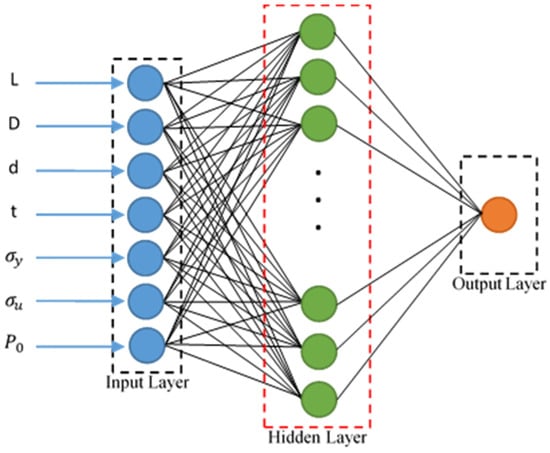
Figure 5.
Structure of ANN for modeling the response of the corroded pipeline LSFs.
Each neuron contains several inputs, with a single output for all of them. The relationship between inputs and output is represented as follows [74]:
where is the weight on the connection for the jth input, is the bias for the hidden layer neurons, T is the number of inputs, () is the activation function. The activation function is usually chosen from a list of S-shaped functions like sigmoid, hyperbolic tangent, or similar functions [75]. If the transposition matrix of inputs and outputs is considered to be as and for an ANN with a hidden layer and m neurons, the output is expressed as follows:
where is the weight of ith neuron in the hidden layer to jth neuron in the output layer, is a constant, (X) is the output of ith neuron in the hidden layer, which is expressed as:
where is the weight of kth input variable in the input layer to ith neuron in the hidden layer, bi is a constant.
4. Illustrative Examples
This section describes three candidate case studies used for the investigation of the performance and efficiency of the above-reported approaches for the accurate estimation of the failure probability for corroded pipelines. Three grade pipelines with low (i.e., X52), mid (i.e., X65), and high (i.e., X100) steel strength were chosen for this purpose, where the statistical properties of the basic random variables and their distributions are detailed in Table 1. As mentioned in Table 1, the burst failure mode of corroded pipeline includes eight random variables with four different distributions as Normal (i.e., D, t,, d, L and P0), Lognormal (i.e., and ), Gumbel (i.e., ), and Freschet (i.e., ). The candidate pipelines have different ranges of design (i.e., D and t) and material (i.e., and ) parameters, although the material characteristic distributions may alter as the pipeline ages (i.e., elapsing time) [76]. The mean of these parameters was taken as the nominal values of the real-cases pipelines (X52, X65, and X100), while a low coefficient of variation (COV) value was given to consider the uncertainties of the manufacturing or human measuring error, whereas the attributed distributions are based on the works of [36,48]. In this work, the corrosion defect depth is suggested to be varied in a range of 15% t to 75% t to account for the degree of severity of the defects at different growth stages. The mean value of corrosion defect length is set to be 200 mm with a normal distribution as suggested by [36,77]. The operating pressure varies between 5 to 25 MPa, where its fluctuations are modelled by a normal distribution and a COV of 0.1 as referred in [44]. The model error distributions and values were adopted based on the works of Mohamed El Amine et al. [36].

Table 1.
Descriptive statistical properties of the candidate pipelines’ random variables.
5. Results and Discussion
This part analyzes and discusses the reliability study performed on the three pipelines (i.e., X52, X65 and X100) presented in Section 4 using the aforementioned simulation and meta-model methodologies. The outcomes are presented in terms of the reliability index (ꞵ), failure probability (Pf), and the number of call-functions (g-call). It is worth noting that the reliability index (ꞵ) and failure probability (Pf) have an inverse relationship based on the standardized normal distribution, as shown in Equation (21).
5.1. Monte Carlo Simulation Accuracy
The Monte Carlo Simulation (MCS) is chosen as the reference technique against which all other methods’ performance will be assessed. This is due to the accuracy of this approach for calculating the failure probability (Pf) when the number of simulations supplied is adequate to cover all conceivable areas based on the LSFs. However, this will incur significant computational expenses. As a result, determining the optimal number of simulations for completing the reliability analysis is critical. In general, the coefficient of variation (CoV) is utilized as an indicator for illustrating the stability of the MCS performance. For simple LSFs, a value of less than 5% is necessary for stable and reliable results using the MCS; consequently, in our study, because the LSFs are highly nonlinear, the required value of CoV is set to be less than 0.0005, and Equation (22) represents the procedure for estimating the CoV for the MCS as follows:
Figure 6a shows how the failure probability varies with the number of simulations for the three selected pipelines (i.e., X52, X65, and X100), while Figure 6b shows the corresponding CoV values. During the analysis, the following mean values of defect geometries and operating pressure were considered: d/t = 0.45; L = 200 mm; and P0 = 10 MPa. As it can be observed, all of the reliability analysis results in terms of failure probability are more stable and produce the same outcomes when no fewer than 106 simulations are used. According to Figure 6b, the values of CoV naturally decrease as the number of simulations increases. Using the 0.0005 threshold condition, the least number of simulations necessary to obtain correct MCS results using the aforementioned basic random variables (i.e., d/t = 0.45; L = 200 mm; and P0 = 10 MPa) is 106. The achieved failure probabilities using 106 simulations are and , with corresponding CoV values of and , respectively. Another observation is that the X65 pipeline provides a higher probability of failure than the X52 pipeline. This is due to the selected basic random variables in Table 1, where the X52 presents a pipeline with a relatively large wall-thickness and diameter (D = 914.4 mm, t = 20.6 mm) compared to the X65 pipeline (D = 762 mm, t = 17.5 mm). Overall, 106 simulations were chosen to perform the reliability analysis findings, utilizing MCS.
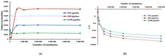
Figure 6.
The effect of simulation number on the reliability outcomes, (a) failure probability versus simulation number (N); (b) CoV versus simulation number (N).
5.2. Performance Evaluation of the Simulation Method
The reliability analysis results for the three corroded pipelines are performed utilizing the four simulation-based methodologies (IS, SS, DS, and LS) and compared to the MCS. Table 2 summarizes the findings of the reliability analysis in terms of failure probability and the needed number of g-call functions, while Figure 7 depicts the fluctuation of the reliability index versus the operating pressure for the X52, X65, and X100 pipelines, respectively. When compared to the required simulation number utilizing the MCS, it is clear that all of the other simulation-based techniques require fewer g-calls, but their performance is reflected in a different manner. To begin, Figure 7 shows that the probability of failures (Pf) decreases as the operating pressure (P0) increases, which is acceptable given the effect of this parameter on the strength condition of corroded pipelines. However, based on the table and figure findings, this is not the case for Pf values produced using the DS and LS techniques for the X52 and X65 pipelines, where results are chaotic and inaccurate. The DS technique was unable to solve the problem for the X100, which may be attributed to the approach’s failure to identify the direction vector since the given LSF of the high strength pipeline is complicated and extremely nonlinear. IS only needed 15,000 simulations to achieve Pf values, however the results are less accurate. SS technique appears to produce the most reliable and accurate results among the other simulation approaches by attaining good Pf values with minimal g-call, which varies between 57,000 and 6000 for low to high Pf values. According to the results of SS, when it comes to low failure probability instances, such as P0 = 5 MPa for the three examples, the needed number of simulations utilizing MCS must greatly rise to at least 1012, resulting in a high computational burden.
Table 2.
Comparative reliability analysis results using simulation methods at various operating pressures and a mean of corrosion defect geometries of d/t = 0.45 and L = 200 mm.
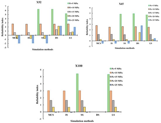
Figure 7.
Variation of the reliability index values corresponding to various operating pressures using simulation-based approaches.
The failure probability and reliability index are also explored in relation to varied corrosion depth-to-wall-thickness (d/t) ratios. The reliability analysis findings are presented in Table 3 in terms of failure probability and g-call, and are displayed in terms of the reliability index, as illustrated in Figure 8. It can be seen that the Pf values decrease as the corrosion depth increases. This comment has previously been shown via various studies, in which findings indicated that the corrosion depth is the key factor reducing pipeline strength as it directly reduces the thickness of the pipe-walls. Unlike findings obtained by varying the operating pressure, simulation-based techniques produced more accurate Pf values for varying the corrosion defect depths. This can be attributed to the comparatively high achieved Pf values by varying d/t to varying the operating pressure. As a result, all methods use fewer g-call functions. As an example, for d/t = 0.15, the Pf values for the X52, X65, and X100 pipelines are 1.83 × 10⁻⁴, 9.96 × 10⁻⁴, and 1.77 × 10⁻⁴, respectively, but for P0 = 5 MPa, the MCS was unable to reliably establish the Pf values due to a lack of simulations. Regardless of the efficiency of the simulation approaches, DS techniques fail to produce any findings for the X100 pipeline for the same reasons stated previously. On the other hand, the LS approach produced the fewest g-calls, followed by the SS strategy, which produced correct results.
Table 3.
Comparative reliability analysis results using simulation methods at various corrosion depth to wall-thickness ratios and a mean of operating pressure P0 = 10 and corrosion length L = 200 mm.
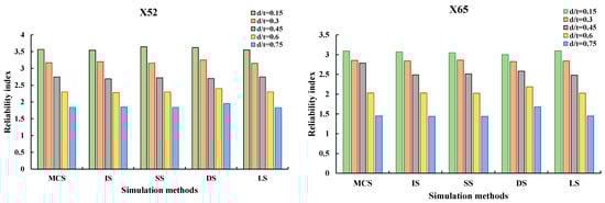
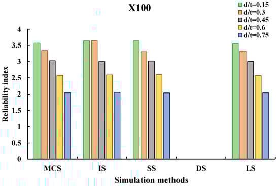
Figure 8.
Variation of the reliability index corresponding to various corrosion depth to wall-thickness ratios using simulation-based approaches.
5.3. Performance Evaluation of the Meta-Models
The reliability analysis findings employing the meta-models and their performance are listed in Table 4 and Table 5 in terms of operating pressure and corrosion-to-wall-thickness ratios, respectively, as in the preceding section. Furthermore, the reliability index values are shown in Figure 9 and Figure 10 in the same respect for the X52, X65, and X100 pipelines. It is worth noting that the kriging-MCS and ANN-MCS algorithms were only assigned 600 g-call functions in order to show their level of accuracy. In terms of the operating pressure, it is discovered that both procedures may obtain acceptable results for P0 over 10 MPa for the three pipelines, indicating that these techniques are highly efficient when compared to the needed g-call using simulation-based methods. It has been observed that the meta-models cannot reach correct solutions when the failure probability is low, as in the case of P0 = 5 MPa. This disadvantage can be mitigated by further adjusting the meta-models’ governing parameters. Overall, the findings of the reliability analysis obtained using meta-models and presented in Figure 9 are similar to those obtained using MCS. The same statements are made in the case of corrosion depth variation, where findings show that the performance of both meta-models is adequate, with greater accuracy utilizing the ANN-MCS technique.
Table 4.
Comparative reliability analysis results using meta-models at various operating pressures and a mean of corrosion defect geometries of d/t = 0.45 and L = 200 mm.
Table 5.
Comparative reliability analysis results using meta-models at various corrosion depth to wall-thickness ratios and a mean of operating pressure P0 = 10 and corrosion length L = 200 mm.
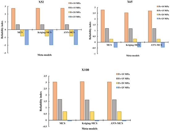
Figure 9.
Variation of the reliability index values corresponding to various operating pressures using meta-models-based approaches.
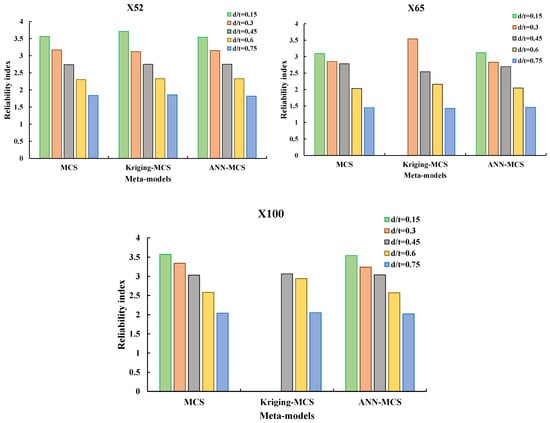
Figure 10.
Variation of the reliability index values corresponding to various corrosion depth to wall thickness ratios using meta-models-based approaches.
5.4. Relative Error in Comparison to Monte Carlo Simulation
The last part explores and discusses the relative error percentage of the failure probability provided by the best simulation and meta-models approaches when compared to the reference approach (i.e., MCS). This cover IS and SS as simulation methods, as well as Kriging-MCS and ANN-MCS as meta-models. Figure 11a,b illustrate the computed relative error percentage plotted in terms of operating pressures and corrosion to wall thickness ratios. The lower the yielded relative error (%), the more accurate the approach’s failure probability outcomes. According to the acquired results, in terms of simulation-based techniques, the SS method produces results with lower relative error (%) than the IS method, and it is also more accurate in estimating lower failure probability than the IS method. As a result, it is possible to infer that, among simulation-based methods, SS may be a viable option for tackling corroded pipeline problems with lower computing costs. ANN-MCS, on the other hand, provides the least relative error compared to all other techniques, indicating its ability to obtain correct results at the lowest computational cost compared to all other approaches. In terms of operating pressures and d/t ratios, ANN-MCS generated a relative error (%) that varies between [0.27–0.8] and [0.36–1.3] for the X52 pipeline, [0.67–2.9] and [0.68–2.9] for the X65 pipeline, and [0–3.7] and [0.38–2.9] for the X100 pipeline. It is possible to infer that employing meta-models is an optimal choice for assessing the safety levels of corroded pipes with low computing effort.
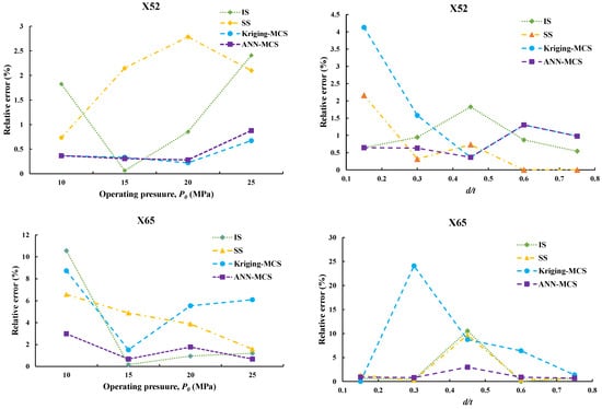
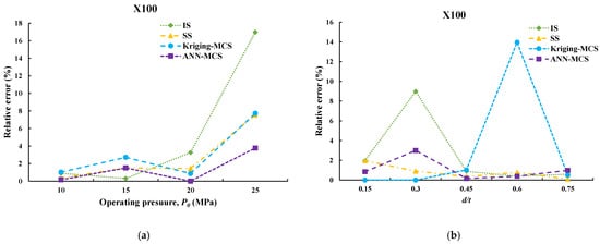
Figure 11.
Estimated relative error percentage using simulation and meta-models (a) versus operating pressures, (b) versus corrosion to wall-thickness ratios.
6. Conclusions
We investigated several simulation and meta-model-based methodologies for the reliability evaluation of corroded pipelines with the collapse failure mode. The suggested approaches investigate the problem from the standpoint of steel strength, with distinct limit state functions given dependent on the pipeline steel grade. This comprises probabilistic burst pressure models for pipelines constructed of low, medium, and high strength steel grade. As a result, sophisticated limit-state functions are presented for calculating the failure probability. The efficiency and accuracy of five simulation methods, including Monte Carlo Simulation (MCS), importance sampling (IS), subset simulation (SS), directional simulation (DS), and line sampling (LS), as well as two meta-models, including kriging and artificial neural network (ANN)-based MCS, for solving the corroded pipeline problem are then investigated.
The suggested techniques’ performance is demonstrated by three corroded pipelines representing low (i.e., X52), medium (i.e., X65), and high (i.e., X100) strength grade steel. To demonstrate the performance of the techniques, crucial factors in the limit-state function, such as corrosion defect depths and the operating pressure, were adjusted from the safest to the most dangerous scenarios. Furthermore, the likelihood of failures due to the collapse failure is evaluated using MCS with various simulation numbers to assess its accuracy based on coefficient of variation criterion. A comparison based on the failure probability, reliability index, g-call, and relative error outcomes has been given. The following are the study’s principal findings:
- Although the MCS is an accurate technique for assessing the failure probability of corroded pipelines, the simulation offered is quite huge when compared to all other simulation and meta-model approaches.
- The risk of collapse failure of the three pipelines is shown to be more sensitive to changes in operating pressure. Obtaining the failure probability for specific operating pressures was discovered to be more challenging than adjusting the corrosion defect depths. This is because the operating pressure is the most critical factor in the limit-state functions that describes the load, and therefore any alterations will result in noticeable observations in the probability of failure findings.
- When compared to MCS, subset simulation was shown to be the most accurate simulation-based technique.
- The results showed that meta-models, particularly the ANN-MCS technique, produce very accurate results that match the MCS solutions almost completely. For the three corroded pipes, ANN-MCS has the lowest g-call (600) and the lowest relative error (percentage). Based on the overall results, ANN-MCS is regarded as the best performing technique for accurate reliability analysis of corroded pipes.
The suggested study is expected to be more challenging if nonlinear corrosion growth or finite element analysis-based reliability analysis is taken into account, since the simulation techniques would be combined with such analysis, resulting an increased complexity and processing costs. Future research should study similar circumstances, utilizing enhanced meta-models based on optimal regulating factors using meta-heuristic algorithms. Furthermore, these studies can be transferred to the system-level analyses to evaluate the operational performance of the network, moreover with considerations of redundant components and robustness-oriented design.
Author Contributions
For Conceptualization, methodology, formal analysis, and writing—original draft preparation, M.E.A.B.S.; funding acquisition, validation, writing—review and editing, P.S.; software, validation, writing—original draft preparation, J.J.-A.; writing—original draft preparation, S.O.; visualization, writing—review and editing, X.L. All authors have read and agreed to the published version of the manuscript.
Funding
This research received no external funding. The publication costs are covered by an Institutional Open Access Program (IOAP).
Institutional Review Board Statement
Not applicable.
Informed Consent Statement
Not applicable.
Data Availability Statement
The data presented in this study are available on request from the corresponding author.
Conflicts of Interest
The authors declare no conflict of interest.
References
- Idris, N.N.; Mustaffa, Z.; Ben Seghier, M.E.A.; Trung, N.-T. Burst capacity and development of interaction rules for pipelines considering radial interacting corrosion defects. Eng. Fail. Anal. 2021, 121, 105124. [Google Scholar]
- El-Abbasy, M.S.; Senouci, A.; Zayed, T.; Mirahadi, F.; Parvizsedghy, L. Artificial neural network models for predicting condition of offshore oil and gas pipelines. Autom. Constr. 2014, 45, 50–65. [Google Scholar] [CrossRef]
- Khan, F.; Yarveisy, R.; Abbassi, R. Risk-based pipeline integrity management: A road map for the resilient pipelines. J. Pipeline Sci. Eng. 2021, 1, 74–87. [Google Scholar]
- Bakar, M.A.A.; Mustaffa, Z.; Idris, N.N.; Seghier, M.E.A. Ben Experimental program on the burst capacity of reinforced thermoplastic pipe (RTP) under impact of quasi-static lateral load. Eng. Fail. Anal. 2021, 128, 105626. [Google Scholar]
- Bridge, G.; Özkaynak, B.; Turhan, E. Energy infrastructure and the fate of the nation: Introduction to special issue. Energy Res. Soc. Sci. 2018, 41, 1–11. [Google Scholar]
- Hopkins, P.; Hopkins, P.; Hopkins, P.; Group, P. The Structural Integrity Of Oil And Gas Transmission Pipelines. Elsevier Publ. 2002, 1, 1–62. [Google Scholar]
- Ben Seghier, M.E.A.; Carvalho, H.; Keshtegar, B.; Correia, J.A.F.O.; Berto, F. Novel hybridized adaptive neuro-fuzzy inference system models based particle swarm optimization and genetic algorithms for accurate prediction of stress intensity factor. Fatigue Fract. Eng. Mater. Struct. 2020, 43, 2653–2667. [Google Scholar]
- Shahriar, A.; Sadiq, R.; Tesfamariam, S. Risk analysis for oil & gas pipelines: A sustainability assessment approach using fuzzy based bow-tie analysis. J. Loss Prev. Process Ind. 2012, 25, 505–523. [Google Scholar]
- Hong, H.P.; Zhou, W.; Zhang, S.; Ye, W. Optimal condition-based maintenance decisions for systems with dependent stochastic degradation of components. Reliab. Eng. Syst. Saf. 2014, 121, 276–288. [Google Scholar] [CrossRef]
- Lam, C. Statistical Analyses of Historical Pipeline Incident Data with Application to the Risk Assessment of Onshore Natural Gas Transmission Pipelines. Master’s Thesis, The University of Western Ontario, London, ON, Canada, 2015. [Google Scholar]
- Ben Seghier, M.E.A.; Höche, D.; Zheludkevich, M. Prediction of the internal corrosion rate for oil and gas pipeline: Implementation of ensemble learning techniques. J. Nat. Gas Sci. Eng. 2022, 99, 104425. [Google Scholar]
- El, M.; Ben, A.; Keshtegar, B.; Fah, K.; Zayed, T.; Abbassi, R.; Thoi, N. Prediction of maximum pitting corrosion depth in oil and gas pipelines. Eng. Fail. Anal. 2020, 112, 104505. [Google Scholar] [CrossRef]
- Ben Seghier, M.E.A.; Keshtegar, B.; Taleb-Berrouane, M.; Abbassi, R.; Trung, N.-T. Advanced intelligence frameworks for predicting maximum pitting corrosion depth in oil and gas pipelines. Process Saf. Environ. Prot. 2021, 147, 818–833. [Google Scholar]
- Yu, W.; Song, S.; Li, Y.; Min, Y.; Huang, W.; Wen, K.; Gong, J. Gas supply reliability assessment of natural gas transmission pipeline systems. Energy 2018, 162, 853–870. [Google Scholar]
- Witek, M.; Batura, A.; Orynyak, I.; Borodii, M. An integrated risk assessment of onshore gas transmission pipelines based on defect population. Eng. Struct. 2018, 173, 150–165. [Google Scholar]
- Zhu, X.-K. A comparative study of burst failure models for assessing remaining strength of corroded pipelines. J. Pipeline Sci. Eng. 2021, 1, 36–50. [Google Scholar]
- Adumene, S.; Khan, F.; Adedigba, S.; Zendehboudi, S.; Shiri, H. Offshore pipeline integrity assessment considering material and parametric uncertainty. J. Pipeline Sci. Eng. 2021, 1, 265–276. [Google Scholar]
- Spyridis, P.; Strauss, A. Robustness assessment of redundant structural systems based on design provisions and probabilistic damage analyses. Buildings 2020, 10, 213. [Google Scholar]
- Su, H.; Zio, E.; Zhang, J.; Li, X. A systematic framework of vulnerability analysis of a natural gas pipeline network. Reliab. Eng. Syst. Saf. 2018, 175, 79–91. [Google Scholar]
- Ghosn, M.; Dueñas-Osorio, L.; Frangopol, D.M.; McAllister, T.P.; Bocchini, P.; Manuel, L.; Ellingwood, B.R.; Arangio, S.; Bontempi, F.; Shah, M. Performance indicators for structural systems and infrastructure networks. J. Struct. Eng. 2016, 142, F4016003. [Google Scholar]
- Gong, C.; Frangopol, D.M. An efficient time-dependent reliability method. Struct. Saf. 2019, 81, 101864. [Google Scholar]
- Bagheri, M.; Zhu, S.-P.; Ben Mohamed El Amine, B.S.; Keshtegar, B. Hybrid intelligent method for fuzzy reliability analysis of corroded X100 steel pipelines. Eng. Comput. 2020, 37, 2559–2573. [Google Scholar] [CrossRef]
- Zhu, S.-P.; Keshtegar, B.; Ben Seghier, M.E.A.; Zio, E.; Taylan, O. Hybrid and enhanced PSO: Novel first order reliability method-based hybrid intelligent approaches. Comput. Methods Appl. Mech. Eng. 2022, 393, 114730. [Google Scholar]
- Gong, C.; Zhou, W. First-order reliability method-based system reliability analyses of corroding pipelines considering multiple defects and failure modes. Struct. Infrastruct. Eng. 2017, 2479, 1451–1461. [Google Scholar] [CrossRef]
- Lee, O.S.; Kim, D.H. The reliability estimation of pipeline using FORM, SORM and Monte Carlo simulation with FAD. J. Mech. Sci. Technol. 2006, 20, 2124–2135. [Google Scholar] [CrossRef]
- Keshtegar, B.; Zhu, S. Three-term conjugate approach for structural reliability analysis. Appl. Math. Model. 2019, 76, 428–442. [Google Scholar] [CrossRef]
- Ben Seghier, M.E.A.; Bettayeb, M.; Correia, J.; De Jesus, A.; Calçada, R. Structural reliability of corroded pipeline using the so-called Separable Monte Carlo method. J. Strain Anal. Eng. Des. 2018, 53, 730–737. [Google Scholar]
- Valor, A.; Caleyo, F.; Hallen, J.M.; Velázquez, J.C. Reliability assessment of buried pipelines based on different corrosion rate models. Corros. Sci. 2013, 66, 78–87. [Google Scholar] [CrossRef]
- Caleyo, F.; Gonzlez, J.L.; Hallen, J.M. A study on the reliability assessment methodology for pipelines with active corrosion defects. Int. J. Press. Vessel. Pip. 2002, 79, 77–86. [Google Scholar] [CrossRef]
- Larin, O.; Barkanov, E.; Vodka, O. Prediction of reliability of the corroded pipeline considering the randomness of corrosion damage and its stochastic growth. Eng. Fail. Anal. 2016, 66, 60–71. [Google Scholar] [CrossRef]
- Gong, C.; Zhou, W. Importance sampling-based system reliability analysis of corroding pipelines considering multiple failure modes. Reliab. Eng. Syst. Saf. 2018, 169, 199–208. [Google Scholar]
- de Angelis, M.; Patelli, E.; Beer, M. Advanced Line Sampling for efficient robust reliability analysis. Struct. Saf. 2015, 52, 170–182. [Google Scholar] [CrossRef] [Green Version]
- Chakraborty, S.; Tesfamariam, S. Subset simulation based approach for space-time-dependent system reliability analysis of corroding pipelines. Struct. Saf. 2021, 90, 102073. [Google Scholar]
- Shayanfar, M.A.; Barkhordari, M.A.; Barkhori, M.; Barkhori, M. An adaptive directional importance sampling method for structural reliability analysis. Struct. Saf. 2018, 70, 14–20. [Google Scholar] [CrossRef]
- Keshtegar, B.; Miri, M. Reliability analysis of corroded pipes using conjugate HL-RF algorithm based on average shear stress yield criterion. Eng. Fail. Anal. 2014, 46, 104–117. [Google Scholar] [CrossRef]
- El Amine Ben Seghier, M.; Keshtegar, B.; Elahmoune, B. Reliability analysis of low, mid and high-grade strength corroded pipes based on plastic flow theory using adaptive nonlinear conjugate map. Eng. Fail. Anal. 2018, 90, 245–261. [Google Scholar] [CrossRef]
- Keshtegar, B.; Ben Seghier, M.E.A.; Zhu, S.-P.; Abbassi, R.; Trung, N.-T. Reliability analysis of corroded pipelines: Novel adaptive conjugate first order reliability method. J. Loss Prev. Process Ind. 2019, 62, 103986. [Google Scholar]
- Leira, B.J.; Næss, A.; Brandrud Næss, O.E. Reliability analysis of corroding pipelines by enhanced Monte Carlo simulation. Int. J. Press. Vessel. Pip. 2016, 144, 11–17. [Google Scholar] [CrossRef]
- Novák, D.; Vořechovský, M.; Teplý, B. FReET: Software for the statistical and reliability analysis of engineering problems and FReET-D: Degradation module. Adv. Eng. Softw. 2014, 72, 179–192. [Google Scholar]
- Ben Seghier, M.E.A.; Keshtegar, B.; Correia, J.A.F.O.; Lesiuk, G.; Jesus, A.M.P. De Reliability analysis based on hybrid algorithm of M5 model tree and Monte Carlo simulation for corroded pipelines: Case of study X60 Steel grade pipes. Eng. Fail. Anal. 2019, 97, 793–803. [Google Scholar] [CrossRef]
- Abyani, M.; Bahaari, M.R. A comparative reliability study of corroded pipelines based on Monte Carlo Simulation and Latin Hypercube Sampling methods. Int. J. Press. Vessel. Pip. 2020, 181, 104079. [Google Scholar]
- Yu, W.; Huang, W.; Wen, K.; Zhang, J.; Liu, H.; Wang, K.; Gong, J.; Qu, C. Subset simulation-based reliability analysis of the corroding natural gas pipeline. Reliab. Eng. Syst. Saf. 2021, 213, 107661. [Google Scholar]
- Velázquez, J.C.; Hernández-Sánchez, E.; Terán, G.; Capula-Colindres, S.; Diaz-Cruz, M.; Cervantes-Tobón, A. Probabilistic and Statistical Techniques to Study the Impact of Localized Corrosion Defects in Oil and Gas Pipelines: A Review. Metals 2022, 12, 576. [Google Scholar]
- Zhou, W. System reliability of corroding pipelines. Int. J. Press. Vessel. Pip. 2010, 87, 587–595. [Google Scholar] [CrossRef]
- Ben Seghier, M.E.A.; Mustaffa, Z.; Zayed, T. Reliability assessment of subsea pipelines under the effect of spanning load and corrosion degradation. J. Nat. Gas Sci. Eng. 2022, 102, 104569. [Google Scholar]
- Keshtegara, B.; Ben Seghier, M.E.A. Modified response surface method basis harmony search to predict the burst pressure of corroded pipelines. Eng. Fail. Anal. 2018, 89, 177–199. [Google Scholar] [CrossRef]
- Amaya-Gómez, R.; Sanchez-Silva, M.; Bastidas-Arteaga, E.; Schoefs, F.; Munoz, F. Reliability assessments of corroded pipelines based on internal pressure—A review. Eng. Fail. Anal. 2019, 98, 190–214. [Google Scholar]
- Guillal, A.; Ben Seghier, M.E.A.; Nourddine, A.; Corria, J.A.F.O.; Mustaffa, Z.B.; Trung, N.-T. Probabilistic investigation on the reliability assessment of mid-and high-strength pipelines under corrosion and fracture conditions. Eng. Fail. Anal. 2020, 118, 104891. [Google Scholar]
- Melchers, R.E. Importance sampling in structural systems. Struct. Saf. 1989, 6, 3–10. [Google Scholar] [CrossRef]
- Au, S.-K.; Beck, J.L. Estimation of small failure probabilities in high dimensions by subset simulation. Probabilistic Eng. Mech. 2001, 16, 263–277. [Google Scholar]
- Rashki, M.; Miri, M.; Moghaddam, M.A. A new efficient simulation method to approximate the probability of failure and most probable point. Struct. Saf. 2012, 39, 22–29. [Google Scholar]
- Koutsourelakis, P.-S.; Pradlwarter, H.J.; Schueller, G.I. Reliability of structures in high dimensions, part I: Algorithms and applications. Probabilistic Eng. Mech. 2004, 19, 409–417. [Google Scholar]
- Metropolis, N.; Ulam, S. The monte carlo method. J. Am. Stat. Assoc. 1949, 44, 335–341. [Google Scholar]
- Grooteman, F. Adaptive radial-based importance sampling method for structural reliability. Struct. Saf. 2008, 30, 533–542. [Google Scholar]
- Miarnaeimi, F.; Azizyan, G.; Rashki, M. Reliability sensitivity analysis method based on subset simulation hybrid techniques. Appl. Math. Model. 2019, 75, 607–626. [Google Scholar] [CrossRef]
- Tee, K.F.; Khan, L.R.; Li, H. Reliability Analysis of Underground Pipelines Using Subset Simulation. Int. J. Civ. Env. Struct Constr Arch. Eng. 2013, 7, 843–849. [Google Scholar]
- Moarefzadeh, M.R.; Melchers, R.E. Directional importance sampling for ill-proportioned spaces. Struct. Saf. 1999, 21, 1–22. [Google Scholar]
- Nie, J.; Ellingwood, B.R. Directional methods for structural reliability analysis. Struct. Saf. 2000, 22, 233–249. [Google Scholar] [CrossRef]
- Jafari-Asl, J.; Ben Seghier, M.E.A.; Ohadi, S.; Correia, J.; Barroso, J. Reliability Analysis Based Improved Directional Simulation Using Harris Hawks Optimization Algorithm for Engineering Systems. Eng. Fail. Anal. 2022, 135, 106148. [Google Scholar]
- Jafari-Asl, J.; Ohadi, S.; Ben Seghier, M.E.A.; Trung, N.-T. Accurate Structural Reliability Analysis Using an Improved Line-Sampling-Method-Based Slime Mold Algorithm. ASCE-ASME J. Risk Uncertain. Eng. Syst. Part A Civ. Eng. 2021, 7, 4021015. [Google Scholar]
- Depina, I.; Le, T.M.H.; Fenton, G.; Eiksund, G. Reliability analysis with metamodel line sampling. Struct. Saf. 2016, 60, 1–15. [Google Scholar]
- Pradlwarter, H.J.; Schueller, G.I.; Koutsourelakis, P.-S.; Charmpis, D.C. Application of line sampling simulation method to reliability benchmark problems. Struct. Saf. 2007, 29, 208–221. [Google Scholar]
- Ditlevsen, O.; Bjerager, P. Methods of Structural Systems Reliability. Struct. Saf. 1986, 3, 195–229. [Google Scholar]
- Lemaire, M. Structural Reliability; John Wiley & Sons: Hoboken, NJ, USA, 2013; ISBN 111862310X. [Google Scholar]
- Keshtegar, B.; Ben Seghier, M.E.A.; Zio, E.; Correia, J.A.F.O.; Zhu, S.-P.; Trung, N.-T. Novel efficient method for structural reliability analysis using hybrid nonlinear conjugate map-based support vector regression. Comput. Methods Appl. Mech. Eng. 2021, 381, 113818. [Google Scholar] [CrossRef]
- Rashki, M.; Azarkish, H.; Rostamian, M.; Bahrpeyma, A. Classification correction of polynomial response surface methods for accurate reliability estimation. Struct. Saf. 2019, 81, 101869. [Google Scholar]
- Elhewy, A.H.; Mesbahi, E.; Pu, Y. Reliability analysis of structures using neural network method. Probabilistic Eng. Mech. 2006, 21, 44–53. [Google Scholar]
- Gaspar, B.; Teixeira, A.P.; Soares, C.G. Assessment of the efficiency of Kriging surrogate models for structural reliability analysis. Probabilistic Eng. Mech. 2014, 37, 24–34. [Google Scholar]
- Wang, Z.; Shafieezadeh, A. REAK: Reliability analysis through Error rate-based Adaptive Kriging. Reliab. Eng. Syst. Saf. 2019, 182, 33–45. [Google Scholar]
- Kaymaz, I. Application of kriging method to structural reliability problems. Struct. Saf. 2005, 2, 133–151. [Google Scholar]
- Xiao, M.; Zhang, J.; Gao, L.; Lee, S.; Eshghi, A.T. An efficient Kriging-based subset simulation method for hybrid reliability analysis under random and interval variables with small failure probability. Struct. Multidiscip. Optim. 2019, 59, 2077–2092. [Google Scholar]
- Xiao, M.; Zhang, J.; Gao, L. A system active learning Kriging method for system reliability-based design optimization with a multiple response model. Reliab. Eng. Syst. Saf. 2020, 199, 106935. [Google Scholar] [CrossRef]
- Ben Seghier, M.E.A.; Corriea, J.A.F.O.; Jafari-Asl, J.; Malekjafarian, A.; Plevris, V.; Trung, N.-T. On the modeling of the annual corrosion rate in main cables of suspension bridges using combined soft computing model and a novel nature-inspired algorithm. Neural Comput. Appl. 2021, 33, 15969–15985. [Google Scholar]
- Papadopoulos, V.; Giovanis, D.G.; Lagaros, N.D.; Papadrakakis, M. Accelerated subset simulation with neural networks for reliability analysis. Comput. Methods Appl. Mech. Eng. 2012, 223, 70–80. [Google Scholar]
- Hurtado, J.E.; Alvarez, D.A. Neural-network-based reliability analysis: A comparative study. Comput. Methods Appl. Mech. Eng. 2001, 191, 113–132. [Google Scholar]
- González-Arévalo, N.E.; Velázquez, J.C.; Díaz-Cruz, M.; Cervantes-Tobón, A.; Terán, G.; Hernández-Sanchez, E.; Capula-Colindres, S. Influence of aging steel on pipeline burst pressure prediction and its impact on failure probability estimation. Eng. Fail. Anal. 2021, 120, 104950. [Google Scholar]
- Zhang, S.; Zhou, W. System reliability of corroding pipelines considering stochastic process-based models for defect growth and internal pressure. Int. J. Press. Vessel. Pip. 2013, 111–112, 120–130. [Google Scholar] [CrossRef]
Publisher’s Note: MDPI stays neutral with regard to jurisdictional claims in published maps and institutional affiliations. |
© 2022 by the authors. Licensee MDPI, Basel, Switzerland. This article is an open access article distributed under the terms and conditions of the Creative Commons Attribution (CC BY) license (https://creativecommons.org/licenses/by/4.0/).