Article

Experimental Validation of a Double-Deck Track-Bridge System under Railway Traffic

1
Institute of R&D in Structures and Construction (CONSTRUCT), School of Engineering, Polytechnic of Porto, 4200-072 Porto, Portugal
2
Department of Structural Engineering, Federal University of Rio de Janeiro, Rio de Janeiro 21941-90, Brazil
3
Institute of R&D in Structures and Construction (CONSTRUCT), Faculty of Engineering, University of Porto, 4200-465 Porto, Portugal
*
Author to whom correspondence should be addressed.
Sustainability 2022, 14(10), 5794; https://doi.org/10.3390/su14105794
Submission received: 29 March 2022 / Revised: 27 April 2022 / Accepted: 5 May 2022 / Published: 10 May 2022
(This article belongs to the Special Issue Sustainable Railway Infrastructure and Rolling Stock)

Abstract

:
This article describes the experimental and numerical evaluation of the dynamic behaviour of the Cascalheira bridge, located on the Northern Line of the Portuguese railway network. The bridge has a short span formed by two filler-beam half-decks, each one accommodating a railway track. The study includes the development of a finite element numerical model in ANSYS® software, as well as in situ dynamic characterization tests of the structure, namely ambient vibration tests, for the estimation of natural frequencies, modes shapes and damping coefficients, and a dynamic test under railway traffic, particularly for the passage of the Alfa Pendular train. The damping coefficients’ estimation was performed based on the Prony method, which proved effective in situations where the classical methods (e.g., decrement logarithm) tend to fail, particularly in the case of mode shapes with closed natural frequencies, as typically happens with the first vertical bending and torsion modes. The updating of the numerical model of the bridge was carried out using an iterative methodology based on a genetic algorithm, allowing an upgrade of the agreement between the numerical and experimental modal parameters. Particular attention was given to the characterization of the ballast degradation over the longitudinal joint between the two half-decks, given its influence in the global dynamic behavior of this type of double-deck bridges. Finally, the validation of the numerical model was performed by comparing the acceleration response of the structure under traffic actions, by means of numerical dynamic analyses considering vehicle-bridge interaction and including track irregularities, with the ones obtained by the dynamic test under traffic actions. The results of the calibrated numerical model showed a better agreement with the experimental results based on the accelerations evaluated in several measurement points located in both half-decks. In the validation process the vertical stiffness of the supports, as well as the degradation of the ballast located over the longitudinal joint between half-decks, was demonstrated to be relevant for the accuracy and effectiveness of the numerical models.

1. Introduction

In the last several decades, several railway administrations have adopted policies of investment focused on the modernization and rehabilitation of existing lines. Although this type of transport is by far more sustainable and environmentally friendly then its competitors, such as air and road transport, this type of upgrade of a railway infrastructure system is accompanied by important challenges, mostly due to the increasing demands in terms of speed and axle loads.
For bridges and viaducts, these new operational demands typically require an accurate evaluation of the dynamic behaviour of the train-track-bridge system to guarantee the structural safety, train running safety and overhead system’s performance as well as passengers’ comfort [1,2,3,4,5,6]. For this purpose, advanced numerical models are developed for the train, track and bridge subsystems, including their interfaces. The accuracy of these models strongly depends on the experimental updating and validation of the numerical results, which is usually performed by means of dynamic measurements based on ambient vibration tests and tests under traffic actions, respectively [3,7,8].
Typically, vehicle-bridge dynamic interaction can be solved using two distinct approaches: coupled or uncoupled [9]. In the first, the vehicle and structure are modelled as a coupled system, in which the equations of each subsystem are assembled into a global system of equations solved simultaneously, that generally requires a high computational effort [10,11]. The second approach relies on separate vehicle and bridge models that are solved using a time history direct-integration method or the modal superposition method, in which the two subsystems meet the compatibility of forces and displacements at the contact points within each time-step by an iterative procedure [12].
Concerning the numerical modelling of the vehicle, the most recent computational modelling strategies that can be found in the literature comprise: (i) multibody formulations, in which the vehicle is modelled as a set of rigid bodies, simulating the carbody, bogies and wheelsets, connected through flexible elements that simulate the primary and secondary suspensions [13]; or (ii) Finite Element (FE) formulations, which allows for consideration of the flexibility of the several components of the vehicle, namely the carbody, making possible to include the local vibration effects in the dynamic responses [14,15].
Regarding the numerical models of bridges, the most advanced are typically three-dimensional FE models including the track [7,8,16]. In these models, the ballasted track components, particularly the ballast layer, sleepers and rail pads, are modelled using volume finite elements, while rails are modelled by beam finite elements.
The inclusion of the ballasted track in the numerical models of the bridges has several advantages. Particularly, it: (i) guarantees an efficient distribution of the trains’ axle-loads [17]; (ii) acts as a filter, removing the high-frequency content from the bridge’s dynamic response [18]; (iii) considers the track-bridge composite effect due to the longitudinal shear stress transmission occurring between rails and bridge deck, through the ballast layer [19,20]; (iv) simulates the track continuity between neighbouring decks [21,22]; and (v) considers the damping mechanisms due to energy dissipation on the track components caused by structure-induced movements [23].
With respect to the track-deck composite effect, Battini & Ülker-Kaustell [24], based on in situ experimental tests, evaluated the influence of the increased amplitudes of the vertical accelerations of the deck immediately after the passage of a train, on the decreasing values of the lowest bending natural frequency. This phenomenon is associated with the nonlinear longitudinal behaviour of the track-deck interface under traffic loads, which tends to arise in specific regions along the bridge where sliding between the track and the bridge deck occurs. Similar conclusions were achieved by Rebelo et al. [25], Rigueiro et al. [26] and Ticona Melo et al. [20].
Several authors emphasize the partial continuity effect provided by the track between adjacent decks, particularly for a succession of simply supported spans or adjacent spans belonging to different railway lines, and its relevance for the understanding of the dynamic interaction between decks, in terms of modal properties and dynamic responses. Ticona Melo et al. [8] demonstrated considerable degradation of the ballast in the longitudinal joint between half-decks, essentially due to the movements induced by rail traffic, which reduces the interaction effect between the adjacent half-decks. In addition, the ballast in the transverse joint between consecutive simply supported decks showed some localized degradation, although not as significantly as that verified in the longitudinal joint. A recent work developed by Sánchez-Quesada et al. [22] demonstrated the relevance of the ballast degradation located on the longitudinal joint between two adjacent simply supported decks, each one carrying a single track, on the modal parameters of the bridge. The best adjustment between numerical and experimental frequencies and mode shapes occurred for a degradation scenario where the value of the deformability modulus of the ballast in the lateral direction was approximately 10% of the value in the vertical direction.
Model updating of the track-bridge system involves the iterative adjustment of the model parameters until a reasonable agreement is obtained between the numerical and experimental modal parameters [8,27]. Some of these techniques are automatic and resort to optimization algorithms that minimize an objective function through successive iterations. There are several algorithms that can be used to solve the optimization problem, namely gradient-based algorithms, response surface methods and nature-inspired algorithms (e.g., genetic algorithm, particle swarm optimization, etc.). One key aspect for the optimization’s success is to use a reliable mode paring technique, i.e., the correspondence between each experimentally obtained mode and a numerically derived mode, to guarantee a fast convergence to the optimal solution [28]. Model updating based on limited experimental data represents another challenge to the robustness and efficiency of the updating procedures that researchers must be aware of [8]. In the case of tests on bridges, infrastructure managers often restrain the number of sensors and corresponding locations due to safety requirements.
Model validation involves the comparison of numerical and experimental dynamic responses under traffic actions. Zhai et al. [29] presented the validation of several numerical models of train-bridge coupling systems using experimental data obtained in trains and bridges belonging to the Chinese high-speed railway network. The authors validate not only the dynamic response of bridges (lateral and vertical accelerations), but also the dynamic response of instrumented vehicles running over those bridges. Ticona Melo et al. [8] carried out the validation of a numerical model of a viaduct composed by four simply supported short spans. After performing the model updating using genetic algorithms based on limited experimental data, the authors compared both vertical displacements and accelerations, measured at one third of the span with displacements transducers and accelerometers, respectively, with the corresponding numerical responses obtained with a train-bridge interaction method. A good agreement was obtained, especially with the numerical model obtained after the updating process. According to several researchers, the match between numerical and experimental data can be improved by taking into account in the numerical model several aspects that may influence the structural response, such as the adoption of experimentally obtained damping coefficients instead of using normative ones [27], the incorporation of elements that could simulate the soil-structure interaction behaviour [7], the consideration of track irregularities in the dynamic model [8], the inclusion of the deformability of the support bearing and their mobility conditions [27] and the inclusion of the track itself in the numerical model of the bridge [26].
Thus, this study aims to give clear contributions in relation to some aspects that presently, according to the authors’ knowledge, are not sufficiently addressed in the existent literature, particularly:
-
Development of an advanced methodology capable of characterizing the degradation of the continuous ballast layer over bridges, particularly in the longitudinal joints between adjacent decks of double-deck bridges. In these specific zones, the ballast is subjected to cyclic movements induced by rail traffic, which can significantly reduce the interaction effect between adjacent decks. The two-step proposed methodology consists, first, of a model updating strategy based on experimental modal parameters and using a genetic algorithm, and second, of a validation strategy to evaluate the robustness of the calibrated model in adequately simulating the dynamic response of the bridge for the train passages. An important contribution of this work is the validation of the dynamic responses on the deck carrying the passing train, as well as on the neighbourhood half-deck, which represents a challenge in terms of the model accuracy and efficiency.
-
The accurate characterization of the level of degradation of the ballast over the joint between half-decks, due to the cyclic shear strain induced by traffic loads, involves the use of a dedicated shear modulus degradation curve, proposed by Ishibashi et al. [30]. This curve can realistically estimate the ballast shear modulus reduction under the high amplitude dynamic displacements that occur during the trains’ passage.
-
The application of the Prony method is used for the estimation of the modal damping coefficients [31]. Comparatively to the classical Logarithm Decrement (LD) method, this method is also based on the free vibration period after the train crossing of the bridge; however, it is more efficient in situations where coupled modes of vibration are present (i.e., modes of vibration with close or very close frequencies). The existence of coupled modes is quite common in short-medium span railway bridges where the natural frequencies of the fundamental torsion and bending modes are close or even merged. The accurate modal damping estimation is decisive for the characterization of the dynamic response of the bridge, particularly in resonances or near resonances scenarios.

2. Numerical Modelling

2.1. Bridge Numerical Model

The Cascalheira bridge (see Figure 1) is a 11.10 m length short-span bridge located at km 100.269 of the Northern Railway Line in Portugal that establishes the connection between Lisbon and Porto. The structure of the deck was completely replaced in 1994, with the aim of increasing the traffic speed. Currently, the maximum allowed speed on this stretch is 160 km/h. The structural solution adopted is a composite filler-beam type, in which the deck is composed of a reinforced concrete slab with embedded steel girders, as shown in Figure 1c.
The cross-section’s width is 11.00 m and consists of two half-symmetrical and independent decks separated by a longitudinal joint. Each half-deck supports a railway track and is composed by nine HEB500 steel profiles, spaced 45 cm apart. The thickness of the concrete slab varies between 0.68 m to 0.76 m from the external extremity to the longitudinal joint. Laterally, the structure comprises two cantilevers with an average thickness of 17 cm that support the sidewalks and serve as retaining walls for the ballast layer. The bearing supports are circular-shaped, located on both sides, under each steel profile. They are composed of an elastomer layer, overlaid by two stainless steel sheets, covered by a vulcanization layer throughout the entire perimeter.
A complex 3D model of the Cascalheira bridge (see Figure 2), including the track, was developed in the finite element software ANSYS® [32]. To better simulate the transition zone in the abutments, an extension of the track was also modeled. Moreover, different materials were used to model the ballast on the longitudinal and transversal joints to allow the study of the degradation of the track in these regions.
Regarding the type of elements adopted to develop the model, shell elements (SHELL63) were used to represent the concrete slabs, cantilevers and the retaining walls, while the embedded steel girders and the rails were modelled with three-dimensional beam elements capable of simulating eccentricities between the modelled position and the real position (BEAM44). Concerning the track, solid elements were used (SOLID45) for the ballast, as well as for the sleepers and rail pads. The non-structural elements, namely the restraining wall, were modelled with concentrated mass elements (MASS21), while the bearing supports were simulated through spring-dashpot elements (COMBIN14) to take into consideration the vertical and longitudinal stiffness of the pot bearings. Finally, rigid beam (MPC184) elements were used to connect the deck to the ballast, and for the connection between the slabs of the deck to the cantilevers and retaining walls. The numerical model had a total of 13,266 finite elements, which contained 15,532 nodes.
The material properties used in the numerical model are shown in Table 1, including the upper and lower limits of variation used for the updating process discussed later in Section 4 and the references consulted to select these limits and part of the statistical properties. For the normal distribution, the limits were calculated by subtracting or adding, to the mean value, two times the value of the standard deviation. The adopted value of the modulus of elasticity of concrete corresponds to the average value of this parameter at the age of 28 days, corrected in order to consider the age of the concrete at the date of the experimental tests (≈26 years), and considering the presence of the steel reinforcement bars. The vertical and horizontal stiffnesses of the supports were initially estimated based in the methodology presented in [33], considering the rubber with a shore hardness of 50. In view of the lack of information regarding the constituent materials of the supports, it was established as the upper limit, the stiffness calculated considering the rubber with a shore hardness of 60, while as the lower limit the 50% degradation of the stiffness was initially considered.
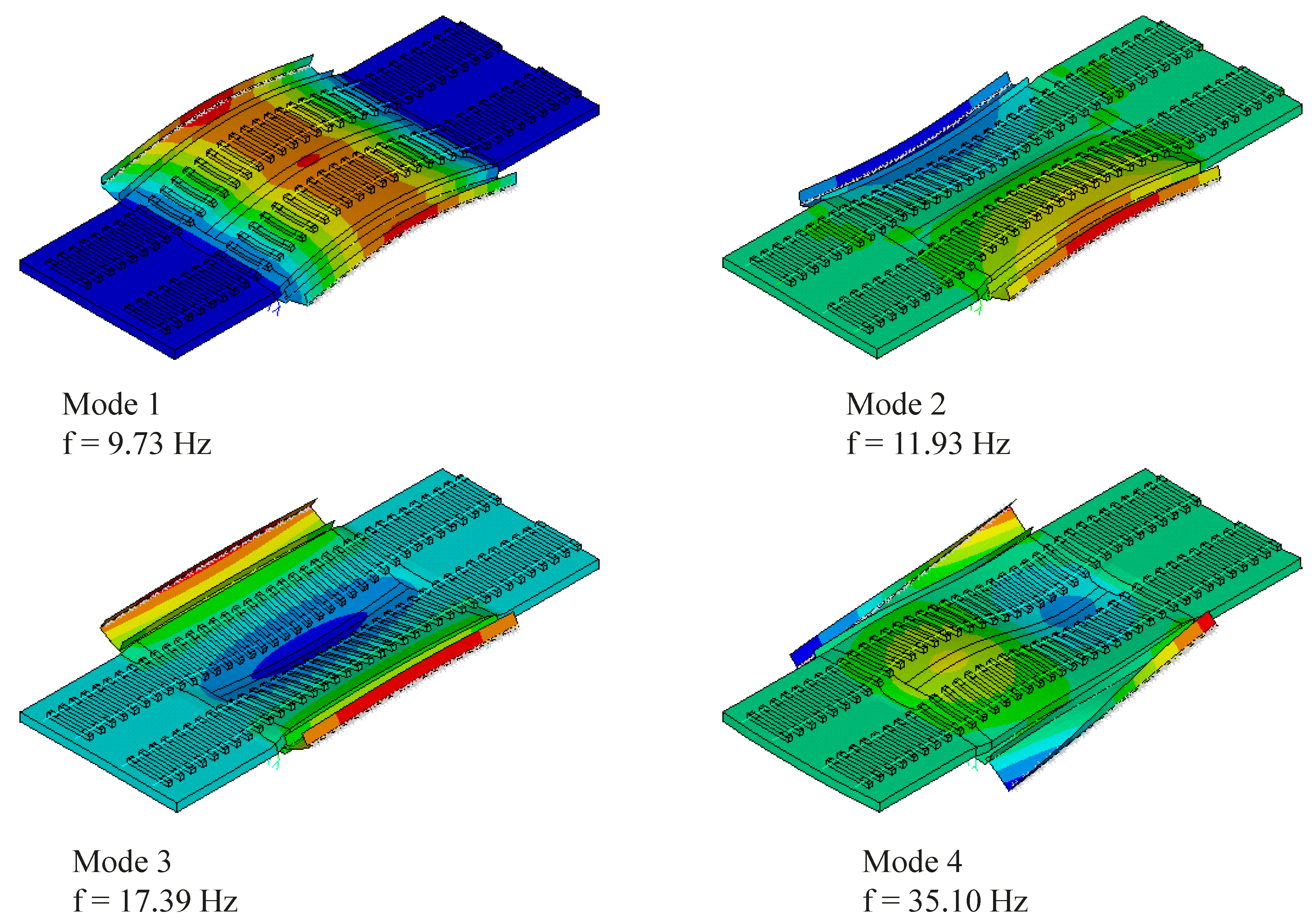
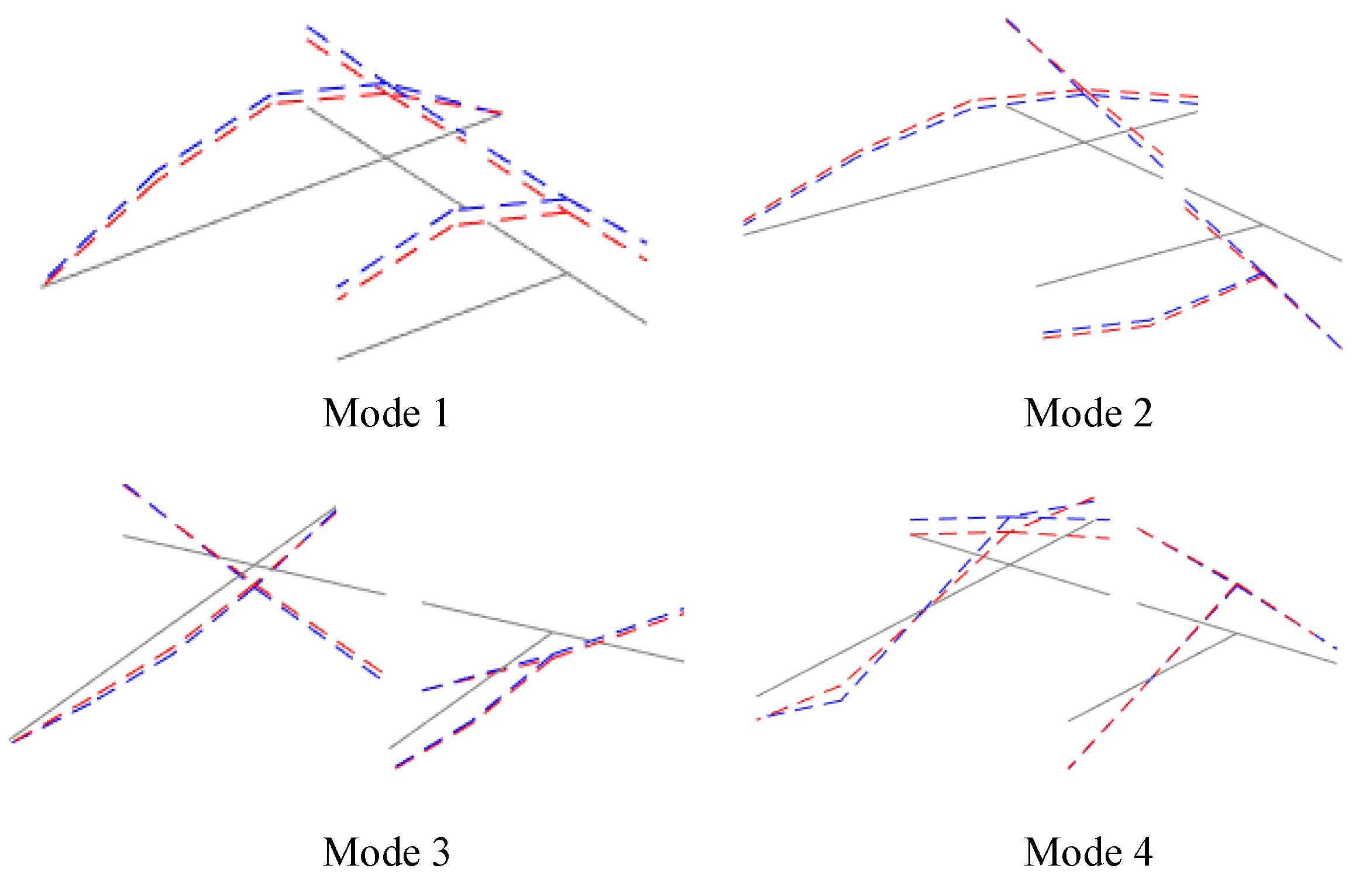
Figure 3 shows the shape of four global vibration modes of the structure and their corresponding natural frequencies, mainly described by bending and torsion movements in the vertical direction. These modes are used in the updating stage of the numerical model described later in Section 4.

2.2. Train Numerical Model

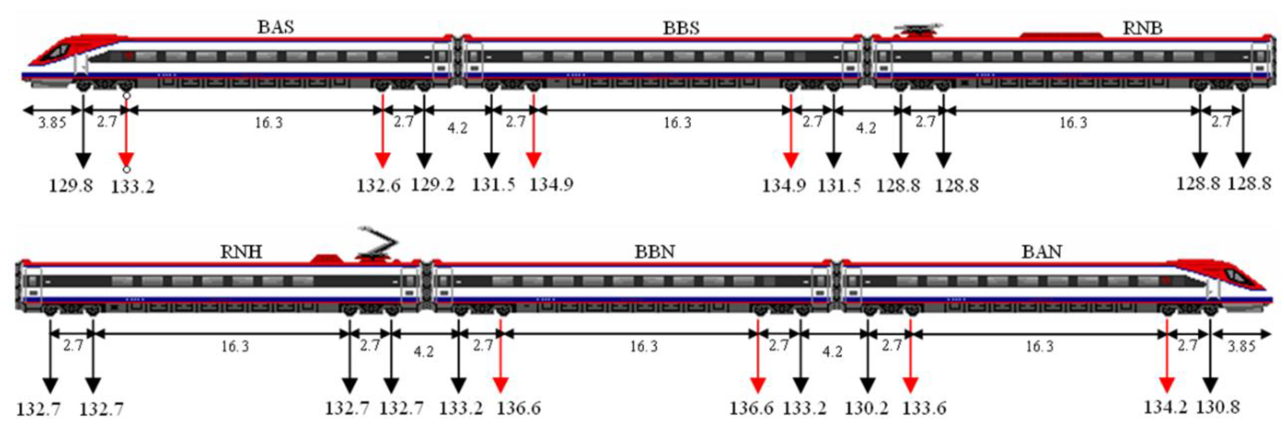
The vehicle considered in this work is the Alfa Pendular train. This conventional train with active tilting system is composed by four motor vehicles (BAS, BBS, BBN and BAN) and two hauled vehicles (RNB and RNH). The train, whose maximum speed is 220 km/h, is 158.9 m long and has a loading scheme composed by 24 axles with loads varying between 128.8 kN and 136.6 kN, as shown in Figure 4. In this figure, the red arrows refer to the motor axles, which are slightly heavier than the non-motor axles represented with black arrows.
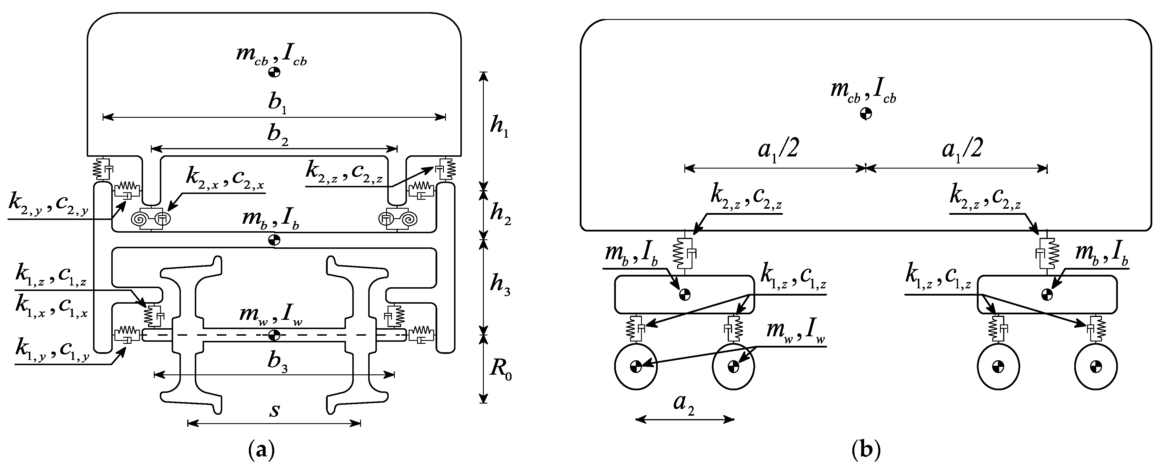
The Alfa Pendular train was modelled using the ANSYS® software [32]. Figure 5 illustrates the dynamic model of one of its cars, including the location of the suspensions and centres of gravity of the different components. In this figure, k, c, m and I represent stiffness, damping, mass and rotational inertia, respectively; a, b and h refer to the longitudinal, transversal and vertical distances, respectively; s represents the gauge and R0 represents the nominal rolling radius. The subscripts cb, b and w refer to the carbody, bogie and wheelset, respectively. Concerning the suspensions, the subscripts 1 and 2 denote the primary and secondary ones, respectively, while the subscripts x, y and z designate the longitudinal, transversal and vertical directions, respectively. All the aforementioned parameters related to the BBN vehicle are presented in Table 2.
For the remaining vehicles, all the parameters previously described are preserved, except the masses that are presented in Table 3. Two values for the bogie masses are assigned, one value when the corresponding bogie has motor and non-motor axles (BAS, BBS, BBN and BAN), the other value when the corresponding bogie has only non-motor axles (RNB and RNH). Regarding the axle masses, an average mass has been considered for simplicity.
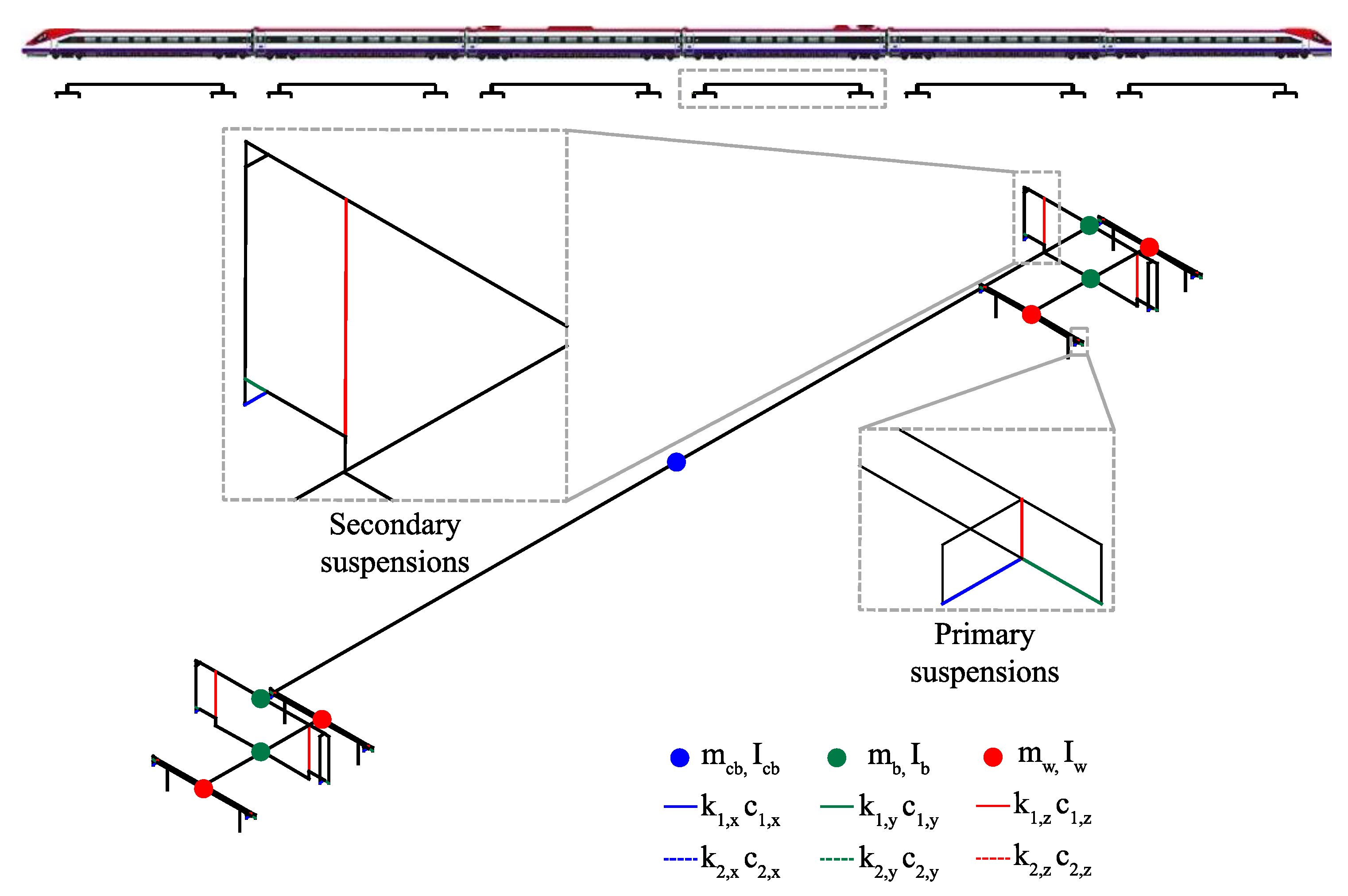
Figure 6 presents an overview of the numerical model developed for the Alfa Pendular train, with a 3D detail of one of its vehicles. The figure shows the rigid elements used to model the carbody, bogies and wheelsets, as well as the concentrated mass elements that simulate their mass and inertia. The primary and secondary suspensions are modelled through spring-dashpot elements (COMBIN14) to take into consideration the stiffness and damping in the longitudinal, transversal and vertical directions.

2.3. Methodology of the Train-Bridge Dynamic Interaction

2.3.1. Wheel-Rail Contact Formulation

In this work, the wheel-rail contact interface is analysed through a specially developed finite element developed, validated and described in detail in Montenegro et al. [40]. According to this contact model, the contact problem is split in three subproblems, namely the geometrical, the normal and the tangential contact problems.
Regarding the first, it consists of determining the contact point position through the parametrization of the contact surfaces, in this case the wheel and rail. To achieve this, a set of geometrical nonlinear equations is solved in each iteration and wheel-rail pair to find the potential contact points. These equations are given by
{ t r · d w r = 0 t w · n r = 0
where t r and t w are the lateral tangential vectors to the rail and wheel surfaces, respectively, at the contact point, d w r is the vector that defines the relative position between the contact points in the wheel and rail surfaces pointing towards the wheel and n r is the normal vector to the rail parametric surface. Figure 7 depicts the physical meaning behind the nonlinear equations for contact search, where it is possible to observe that the potential contact pair may be a valid contact point if the tangent vector to the rail surface is perpendicular to the vector that connects wheel and rail contact points (first equation) and the tangent vector to the wheel is also perpendicular to the normal vector to the rail (second equation). However, these two conditions are not sufficient to guarantee contact, because when vectors d w r and n r point in the same direction, although it also represents a valid mathematical solution, it does not correspond to actual contact (see Figure 7b). Thus, to guarantee contact, an additional condition has to be imposed that can be represented through the following inequation:
d w r · n r 0
The second subproblem consists of determining the normal contact forces that arise between wheel and rail F n when they are compressed against each other. In this model, these forces are computed with the nonlinear Hertz contact theory [41] as
F n = K h   d 3 2
where d is the penetration between the two contact bodies given by the norm of vector d w r and K h   is a generalized stiffness coefficient dependent on the material properties and curvatures of the surfaces of the contacting bodies [42].
Finally, the third subproblem aims to calculate the tangential contact forces, also known as creep forces, that arise from the rolling friction between wheel and rail. In this model, the USETAB [43] algorithm is used to compute these forces. This algorithm takes advantage of an efficient organization of a predetermined lookup table, in which the longitudinal and lateral tangential contact forces can be interpolated during the dynamic analysis as function of the creepages (relative velocities between wheel and rail at the contact point) and the semi-axes ratio of the Hertz contact ellipse.

2.3.2. Dynamic Equations of the Train-Bridge Coupling

The dynamic analyses performed in the present study have been carried out with a train-bridge interaction tool named “VSI—Vehicle Structure Interaction Analysis”, developed by Montenegro et al. [40], in which the train is coupled to the bridge through a set of constraint equations that connects the wheel-rail contact element attached to the vehicle and described in Section 2.3.1 to the track included in the bridge model. These equations are added to the governing equilibrium equations of motion of the train-bridge system, forming a single system with displacements, a, and contact forces, X, as unknowns (Lagrange multipliers method) that can be mathematically described as:
[ K ¯ D ¯ H ¯ 0 ] [ Δ a F i + 1 Δ X i + 1 ] = [ ψ ( a t + Δ t , i , X t + Δ t , i ) r ¯ ]
in which K ¯ is the effective stiffness matrix of the train-bridge system, D ¯ and H ¯ are transformation matrices that relate the contact forces and displacements, respectively, in the local coordinate systems of the contact elements with the global coordinate system, ψ is the vector of residual forces and r ¯ is the vector of track irregularities that exist in the contact interface between wheel and rail. Since the irregularities are directly introduced in the constraint equations, it is not necessary to explicitly incorporate them in the bridge-track FE model described in Section 2.1, which significantly simplifies the track model. Finally, given the nonlinear characteristics of the wheel-rail contact model (see Section 2.3.1), an incremental solution is needed to solve the system of equations described above. Therefore, Δa and ΔX are the incremental nodal displacements and contact forces, respectively, that can be computed through the Newton-Raphson method. Regarding the superscripts, t + Δ t refers to the current time step, while i and i + 1 indicate the previous and current Newton iteration, respectively. The dynamic analysis is solved based on a direct integration scheme based on the α-method [44].
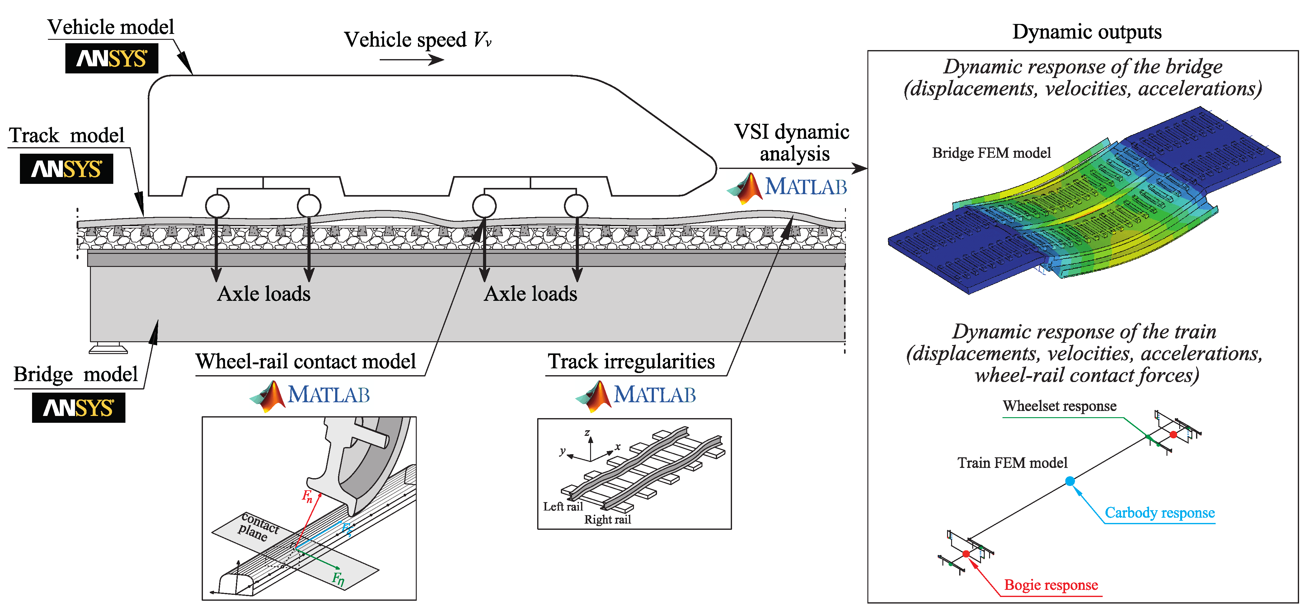
As mentioned before, and although the present work only focuses on vertical dynamics, the train-bridge dynamic interaction tool adopted in this study treats the contact interface through a proper wheel-rail contact model, in which the normal and tangential forces are obtained based on the Hertz nonlinear theory [41] and the Kalker’s USETAB algorithm [43], respectively. This numerical tool, which has been programmed in MATLAB® [45], imports the structural matrices of the bridge and train models developed in a FE package (in this case ANSYS® [32]), allowing the study of structures with any degree of complexity in an efficient way. Figure 8 shows the framework of the VSI tool and the outputs that can be obtained in the dynamic analyses carried out by it. A detailed description of this numerical tool can be consulted in [40].

3. Dynamic Tests

3.1. Ambient Vibration Test

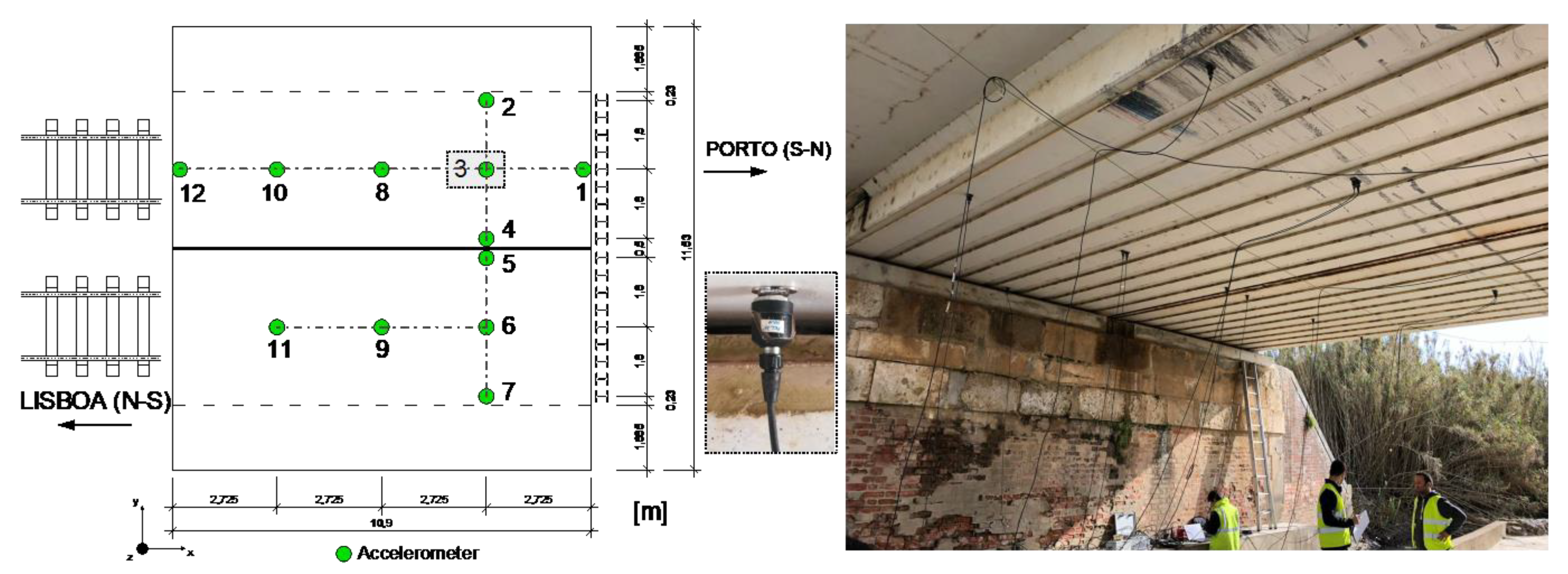
An ambient vibration test was conducted to identify the modal parameters of the bridge, particularly its natural frequencies, mode shapes and modal damping coefficients. A technique based on fixed reference points was adopted, with a test setup based on 12 measurement points, involving the use of piezoelectric accelerometers, PCB model 393B12, with a sensitivity of 10 V/g and a measurement range of ±0.5 g, installed at the lower face of the bridge deck. The time series were acquired in periods of 10 min, with a sampling frequency of 2048 Hz, which was posteriorly decimated to a frequency of 256 Hz. The data acquisition was performed using the cDAQ-9188 system from National Instruments (NI), equipped with IEPE analogue input modules with 24 bit resolution (NI-9234). Since the purpose of this test was to determine the vertical bending and torsion movements, all the accelerometers were installed in the vertical direction.
Due to the low acceleration levels of the deck under ambient actions, in some situations the additional excitation provided by a non-instrumented impact hammer at the lower face of the deck was useful for increasing the amplitude of movement of the deck, leading to an increase of the signal-to-noise ratio and, consequently, to a significant improvement of the signal quality.
Figure 9 illustrates the experimental configuration of the test setup to identify the modal parameters of the bridge deck. The accelerometers were distributed along the span in the centre of each track, with two accelerometers in the lateral extremities of each half-deck used to distinguish the torsion modes from the vertical ones (the dashed-doted gray lines represent the location of the accelerometers, used later in the comparison between experimental and numerical mode shapes). Given the constraints to accessing the upper face of the deck due to traffic, the sensors were installed at the lower face of the deck through magnetic bases, namely on the bottom flange of the steel girders. The cables of the accelerometers were attached to the lower part of the deck using adhesive tape. This strategy allows for avoiding eventual movements of the cables induced by wind, or other external sources, that may influence the vibration responses.
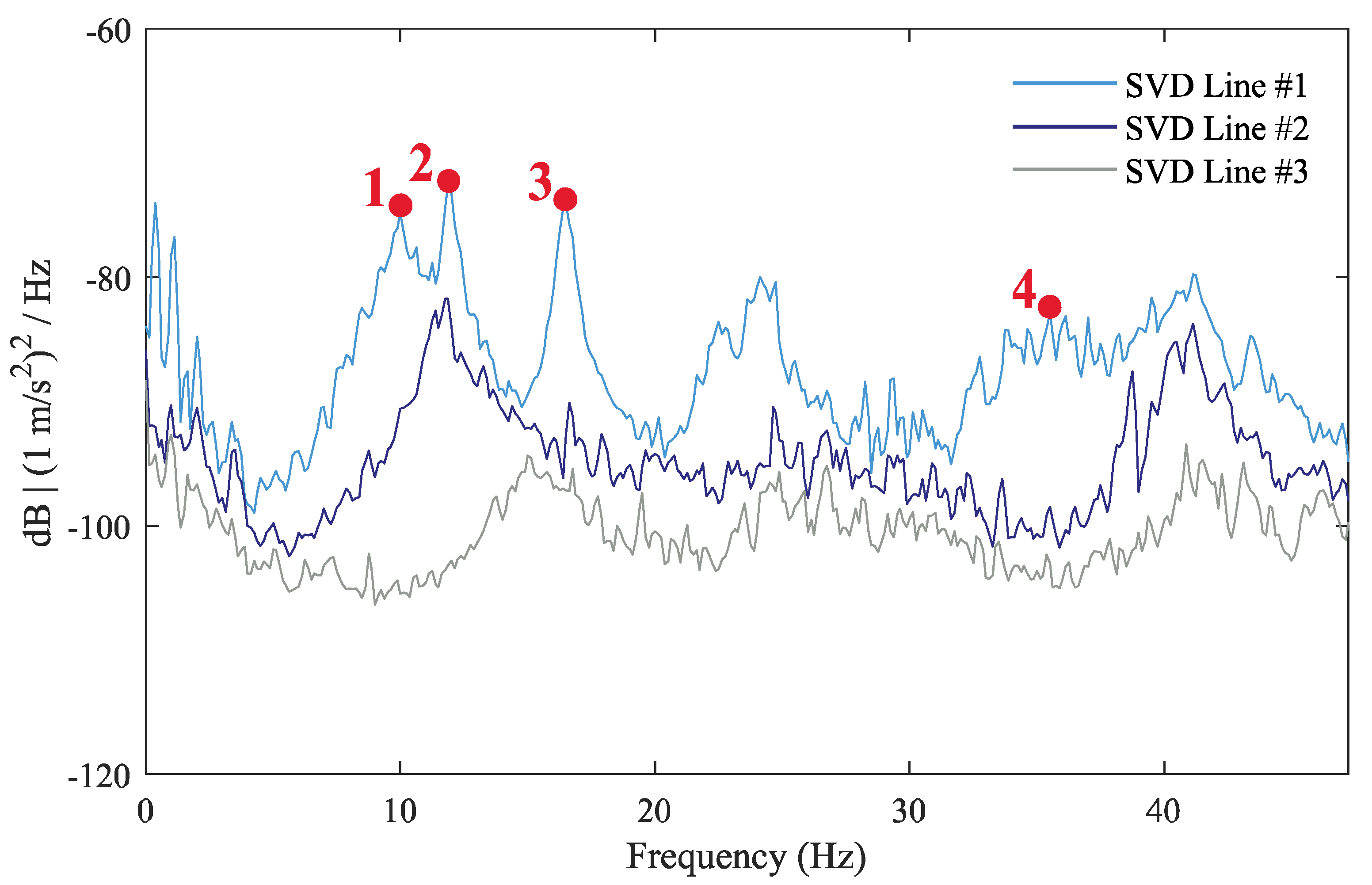
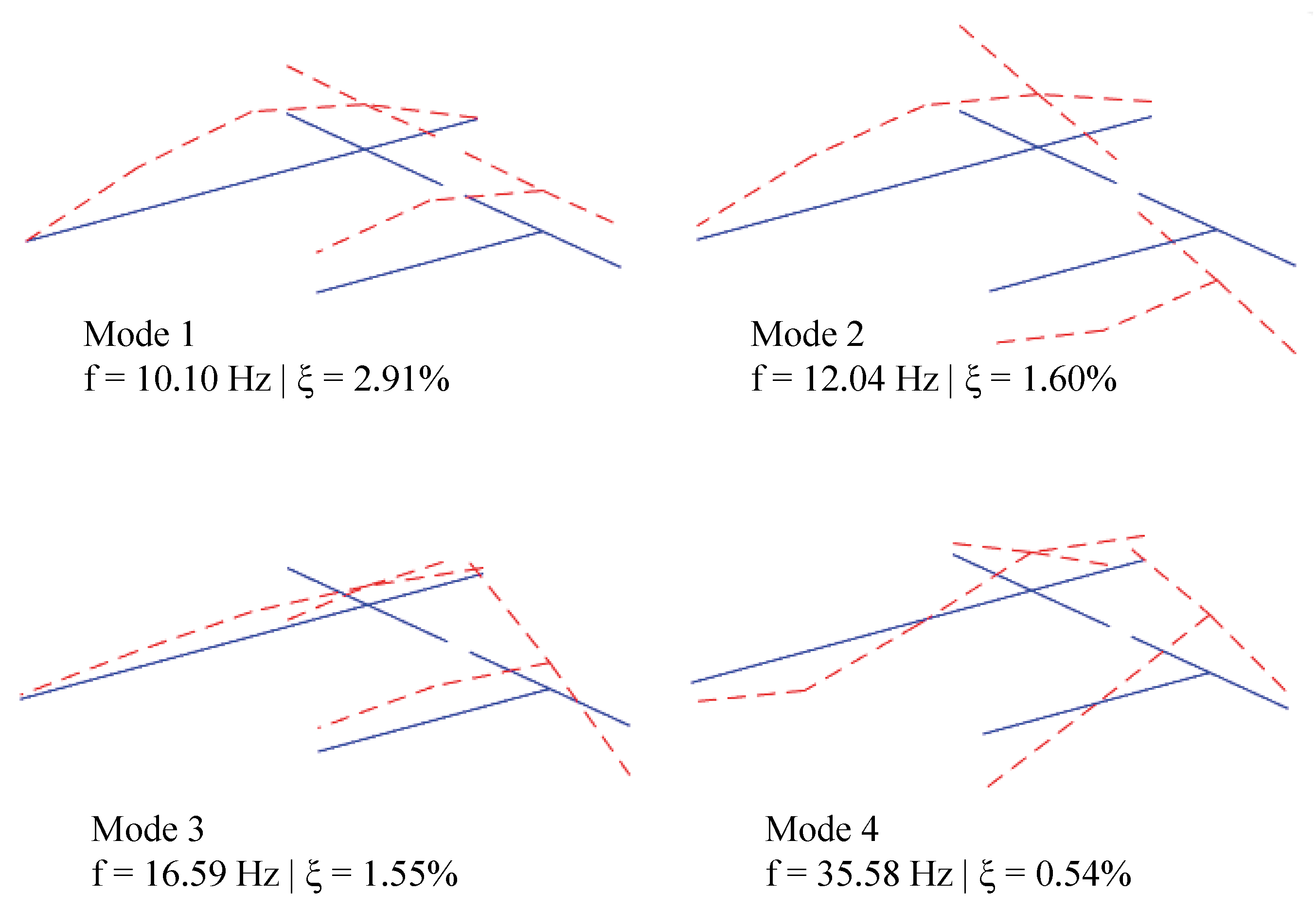
Modal identification was performed using the Enhanced Frequency Domain Decomposition (EFDD) method available in the ARTeMIS® software [46]. In Figure 10, it is possible to observe peaks (red dots) in the first three curves of the average normalized singular values of the spectral density matrices of all test setups, these peaks corresponding to the four identified global vibration modes depicted in Figure 11 (where f is the average value of the natural frequency and ξ is the average value of the damping coefficient).

3.2. Test under Railway Traffic

The tests under railway traffic aimed to measure the dynamic response of the bridge deck in terms of accelerations caused by the passage of trains. These responses were used for estimating the bridge damping, as well as for validating the efficiency of the numerical model in realistically reproducing the dynamic response of the bridge under railway traffic, as will be discussed later in Section 5.
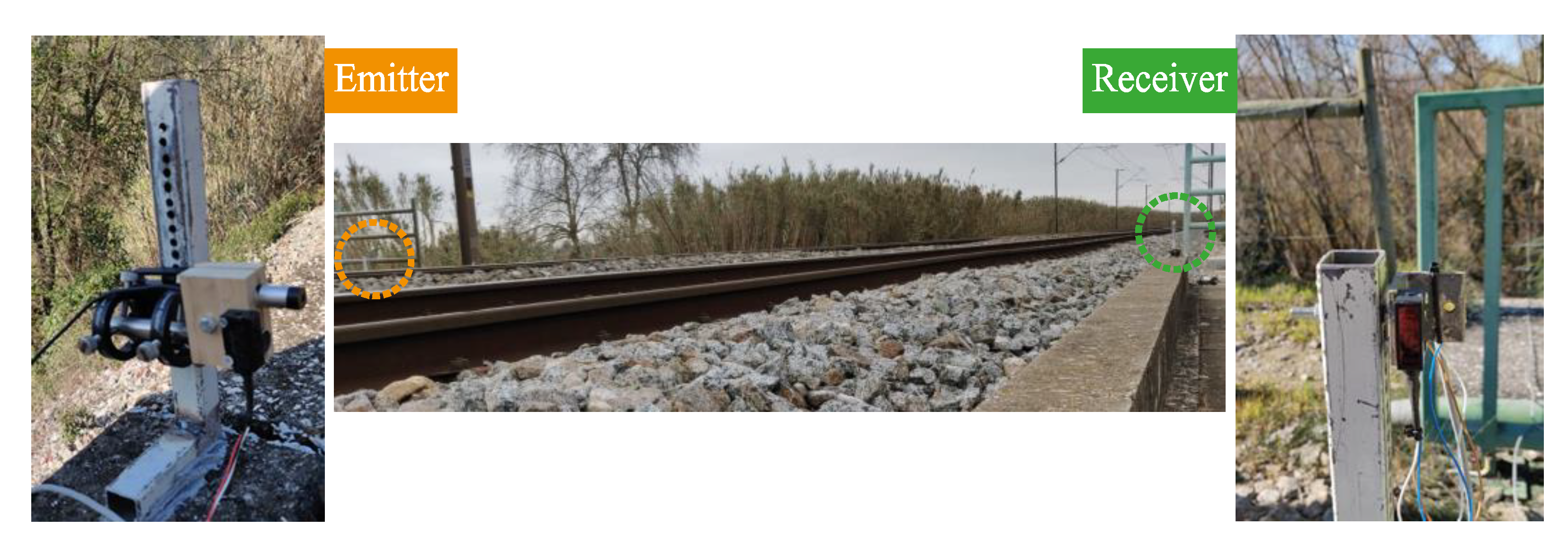
Figure 12 shows the four measurement points located at the lower face of the deck, in which the vertical accelerations were measured using piezoelectric accelerometers, PCB model 393A03, with a sensitivity of 1 V/g and a measurement range of ±5 g. For detecting the train axles, two groups of optical sensors were installed on each bridge extremity, including an emitter and a receiver located on opposite track sides (see Figure 13). These optical sensors allowed the detection of the precise time instant that the last train axle left the bridge, which is decisive when accurately assessing the beginning of the free vibration movement of the bridge, this being necessary for estimating the bridge damping. The data acquisition was performed using the cDAQ-9188 system from National Instruments (NI), equipped with IEPE analogue input modules with 24 bit resolution (NI-9234). The time series were acquired at a sampling rate of 2048 Hz.
The estimation of the damping coefficients was based on the deck’s acceleration responses, caused by the passage of trains, obtained in the two highlighted positions illustrated in Figure 12 (midspan position of each half-deck). For the particular case of the Cascalheira bridge, the free vibration of the structure was not just controlled by the first bending mode but also by the first torsional mode, whose natural frequencies are close to each other (see Figure 11). In these situations, where the natural frequencies of the fundamental bending and torsion modes are close or sometimes merged, which is common in short-span railway bridges, the Prony method has shown significant advantages in the estimation of damping coefficients when compared to the LD method [31]. The Prony method allows for the decomposition of the signal in a set of exponential decaying sinusoids representative of each frequency of interest, while in the LD method this decomposition is not possible since it works on coupled sampled data [47]. More details about the Prony method are available at ERRI D214/RP3 [31] from the ERRI D214 specialists committee.
The Prony method uses free vibration data, y [ t ] , to estimate a complex exponential model of the form [48]:
y [ t ] = i = 1 n A i e ξ i ω 0 , i t cos ( ω 0 , i 1 ξ i 2 + ϕ i )                        
where n is the number of complex exponentials of interest, A i the amplitude of the ith exponential component, ξ i the damping coefficient, ω 0 , i the angular frequency, and ϕ i the phase angle.
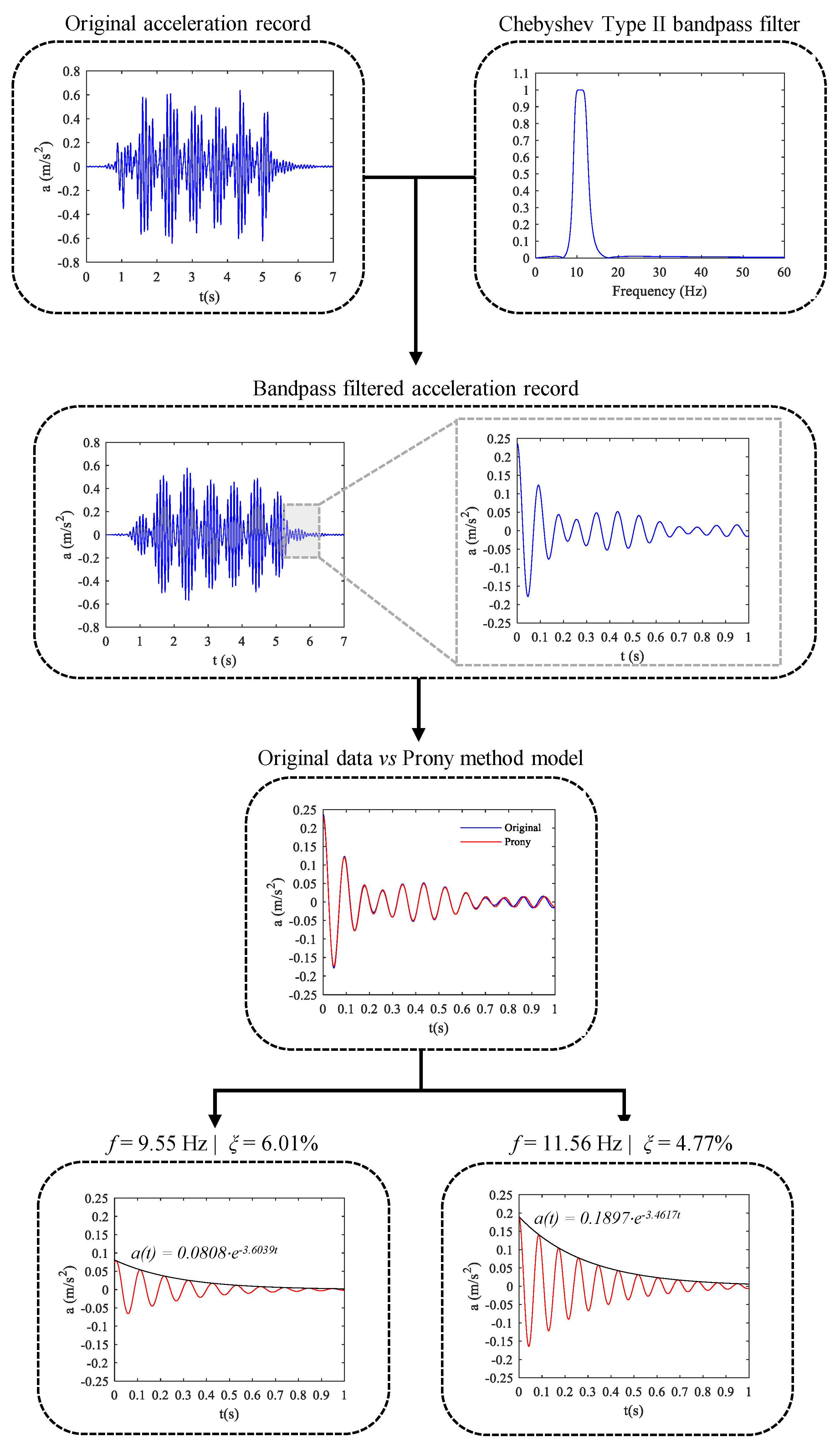
In this work, the methodology for the damping estimation of modes 1 and 2 is summarized in Figure 14 based on the acceleration record derived from the Alfa Pendular train at a speed of 140 km/h. First, the original acceleration records are bandpass filtered to isolate the contributions of modes 1 and 2 on the dynamic response. The filter is a Chebyshev Type II of order 6 with an attenuation band of 40 dB and cut-off frequencies of 7 and 16 Hz, centred between the frequency values of the 1st and 2nd modes of the bridge. Posteriorly, the Prony method is applied to the bandpass filtered free-vibration record. Figure 14 shows the overlapping of the fitted exponential model, derived from the superposition of two exponential sinusoids, with the original sampled data. A very good fitting between the two models was obtained, considering the frequencies and damping coefficients equal to 9.55 Hz/6.01% for mode 1, and 11.56 Hz/4.77% for mode 2.
Table 4 presents the damping coefficient estimates obtained from the Prony method for modes 1 and 2 and considering the passage of the Alfa Pendular train over the bridge at different speeds (110, 135 and 140 km/h). The table also indicates the average damping coefficient values (marked on bold). It can be observed that the damping coefficients obtained for the different train passages are quite similar, proving the efficiency and consistency of the method.

4. Model Updating

The updating of the numerical model of the Cascalheira bridge was performed based on the results of the ambient vibration test and involved two stages: A global sensitivity analysis based on a stochastic sampling technique, and an optimization process based on a genetic algorithm. The mode paring was based on the Model Assurance Criterion (MAC).

4.1. Mode Pairing

The pairing of the numerical and experimental modes was conducted through the MAC parameter, which provides a measure of the linear correlation between the numerical and experimental modal vectors through their mean square deviation [49]. This parameter is a scalar that can vary between 0 and 1, whose unit value indicates that the numerical and experimental values are coincident or linearly dependent. The MAC value can be estimated based on the following expression:
M A C i j = M A C ( Φ i *   ,   Φ j * ) = Φ i * T     Φ j * ( Φ i * T     Φ i * )     ( Φ j * T     Φ j * )
where Φ j * is the vector containing the coordinates from the numerical mode j corresponding to the numerical data and Φ i * the vector containing the experimental information of mode i.
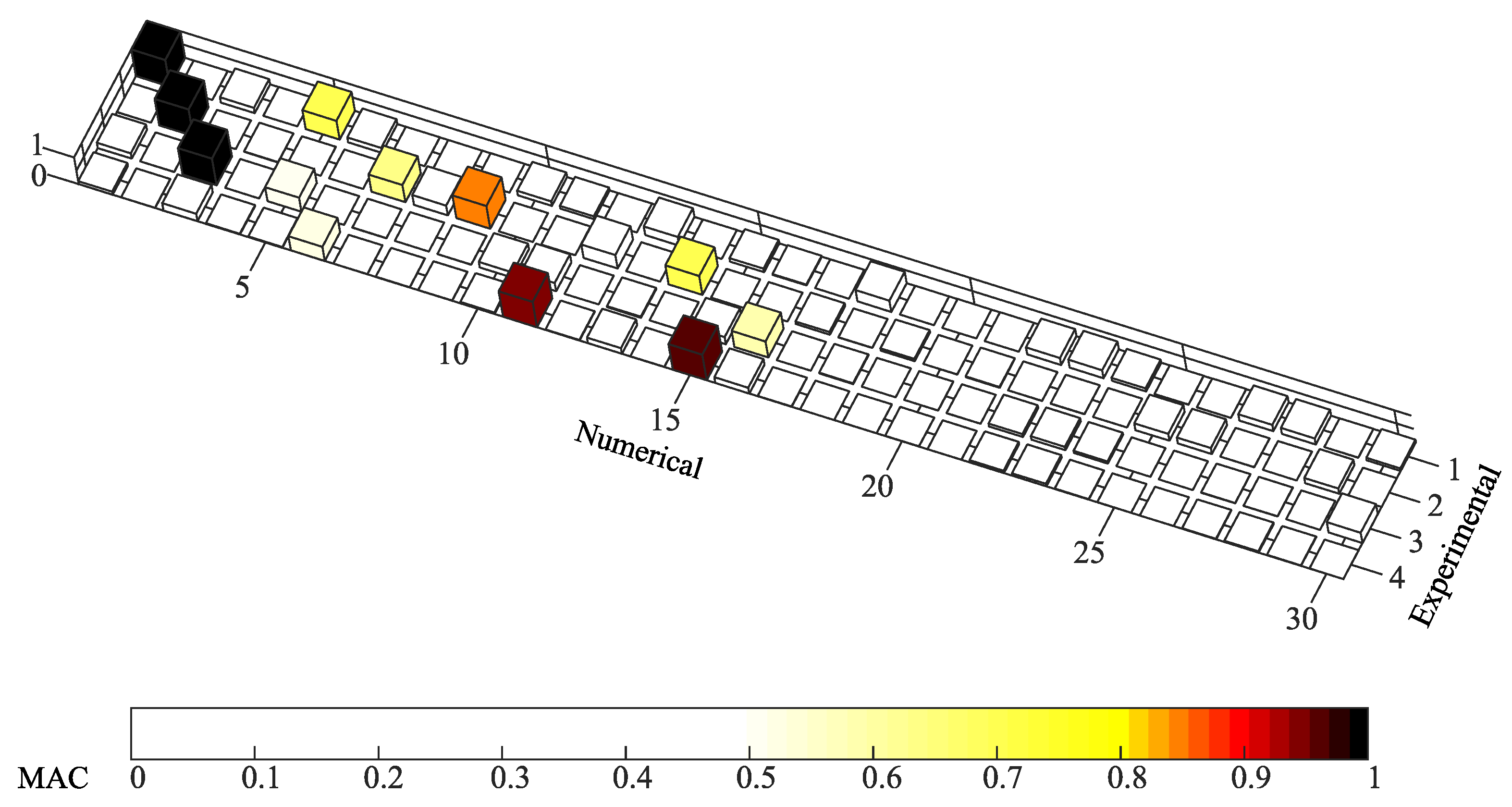
For the initial numerical model, the MAC matrix is shown in Figure 15, where it can be observed that the first three experimental modes have high correlation coefficients with the corresponding numerical modes, while the experimental mode 4 presents a higher correlation with the numerical mode 15. Thus, the results reveal a predictable, stable and consistent mode pairing for the further sensitivity analysis and optimization.

4.2. Sensitivity Analysis

The sensitivity analysis allows the identification of the numerical parameters that most influence the natural frequencies and mode shapes. Only the parameters with significant correlation with the modal responses can be correctly estimated during the optimization process.
Figure 16 presents the Spearman linear correlation matrix between numerical parameters and modal responses, i.e., frequencies and MAC values. The range of variation of the numerical parameters is in accordance with the limits presented in Table 1. The global sensitive analysis was carried out using a stochastic sampling technique based on 750 samples generated by the Latin Hypercube method. The correlation coefficients in the range between −0.30 and +0.30 were excluded from the graphical representation to emphasize the higher correlations. By observing the figure, it is possible to notice that only 5 of the 13 analysed parameters have a significant influence on the modal responses, namely the modulus of deformability (Ec) and density (ρc) of the concrete, the modulus of deformability of the ballast in the longitudinal joint (Ebl), the density of the ballast (ρb) and the vertical stiffness of the supports (Kv).

4.3. Optimization

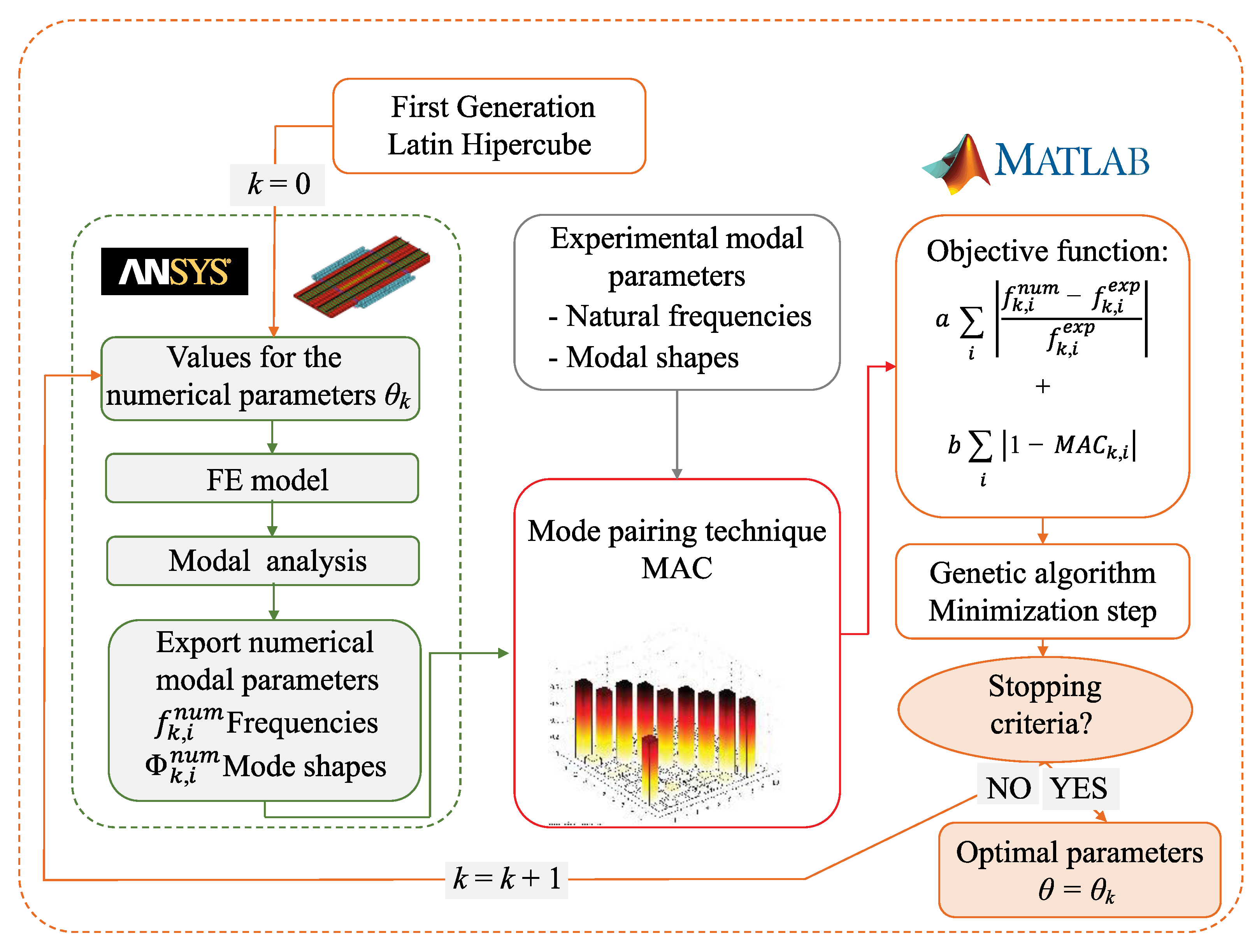
The optimization stage aims at finding the optimal values of the numerical parameters identified through the sensitivity analysis, in order to minimise the differences between the numerical and experimental modal parameters. The automatic optimisation of the numerical model involved an iterative process based on a genetic algorithm and requires the interaction between two pieces of software: MATLAB® [45] and ANSYS® [32] (see Figure 17). A detailed description of the proposed methodology can be found in Ribeiro et al. [14].
The optimization involved five numerical parameters and eight modal responses (four frequencies and four modal configurations). The objective function f o b j involved two terms: the first includes the residuals of the natural frequencies and the second the residual of the mode shapes. This function can be expressed as:
f o b j = a i = 1 4 | f i e x p f i n u m | f i e x p + b i = 1 4 | M A C ( ϕ i e x p , ϕ i n u m ) 1 |
where a and b are the residuals weights assumed equal to 1.0, f i e x p is the frequency of the ith experimental mode, f i n u m is the frequency of the ith numerical mode and M A C ( ϕ i e x p , ϕ i n u m ) is the MAC value between the ith numerical and experimental modal configurations.
The genetic algorithm was based on an initial population of 30 individuals, randomly generated by the Latin Hypercube method, considering 100 generations and totalising 3000 individuals. Each individual represents a specific set of numerical parameters. The crossing rate was considered equal to 50%, the replacement rate equal to 5% with a number of elites per generation equal to 1, and the mutation rate was set equal to 15%, with a variable standard deviation between 0.10 and 0.01. Four independent optimisation runs (GA1 to GA4) with different initial populations were performed to obtain an optimal solution due to the stochastic nature of the genetic algorithms. The total computational time of each optimisation run lasted approximately 13 h on an INTEL Core i5-5200U laptop with 2.20 GHz and 8.00 Gb RAM.
Figure 18 shows the ratios of the numerical parameters in relation to the limits indicated in Table 1 for optimisation runs GA1 to GA4. Additionally, the optimal values of each numerical parameter are also indicated. A ratio of 0% means that the parameter coincides with the lower limit and a ratio of 100% means that it coincides with the upper limit. The values of optimisation run GA2 were adopted as optimal values because they led to the lowest value of the objective function.
Generally, all the parameters showed a small variation for the four optimizations runs. However, parameters that are more sensitive to the responses, e.g., vertical stiffness of the supports (Kv) and density of the ballast (ρb), present a tightness variation of values in the optimization stage. In turn, parameters that are not so sensitive to the responses, e.g., modulus of deformability (Ec) and density (ρc) of the concrete, present a slightly higher dispersion of values in the optimization stage. Regarding the ballast density (ρb), it showed a variation of only 2.2% between optimizations, while the latter presented variations lower than 1.2%. Moreover, it is interesting to notice that the values obtained for the vertical stiffness of the supports are close to the lower limit (average ratio of 9.5%), which indicates a possible degradation of these bearing devices. The modulus of deformability of the concrete (Ec) presented average values close to that adopted in the initial numerical model (average ratio of 50.1%), which indicates that the initial value estimation was satisfactory. Despite the variation of the parameter values between the optimization runs was noticeably low (11.6%), this was the largest variation among the analysed parameters. The modulus of deformability of the ballast in the longitudinal joint (Ebl) showed close values between the first three optimizations and a greater variation in the GA4 optimization. The average ratio obtained was 49.0%, which may indicate a degradation of the longitudinal joint, since the parameter value on the initial model corresponds to its upper limit.
Figure 19a illustrates the error between the numerical frequencies, before and after the updating process, in relation to the corresponding experimental values. For modes 1, 3 and 4, the calibrated model reached natural frequencies practically equal to those obtained experimentally. The only exception is mode 2, for which the numerical frequency value became slightly more distant from the experimental one after the updating. A better match for the frequency of mode 2, a global torsion mode, would probably require the inclusion of additional numerical parameters (e.g., distinct values of the vertical stiffness for the individual supports (or groups of supports), uncertainty of the mass distribution on the cantilevers), and inherently, the consideration of additional measurement points in the regions of the supports and cantilevers. The average error of the frequencies decreased from 2.65% before updating to 0.69% after updating. Figure 19b presents the MAC values before and after updating. The average value of the MAC parameter increased from 0.985 to 0.988, before and after calibration, respectively. This result reveals a very slightly upgrade of the modal configurations with the calibration process; however, the very high MAC values state the excellent match between the numerical and experimental mode shapes, as presented in Figure 20 (the gray lines, which are represented in Figure 9, represent the locations of the accelerometers).

5. Model Validation

5.1. Initial Considerations

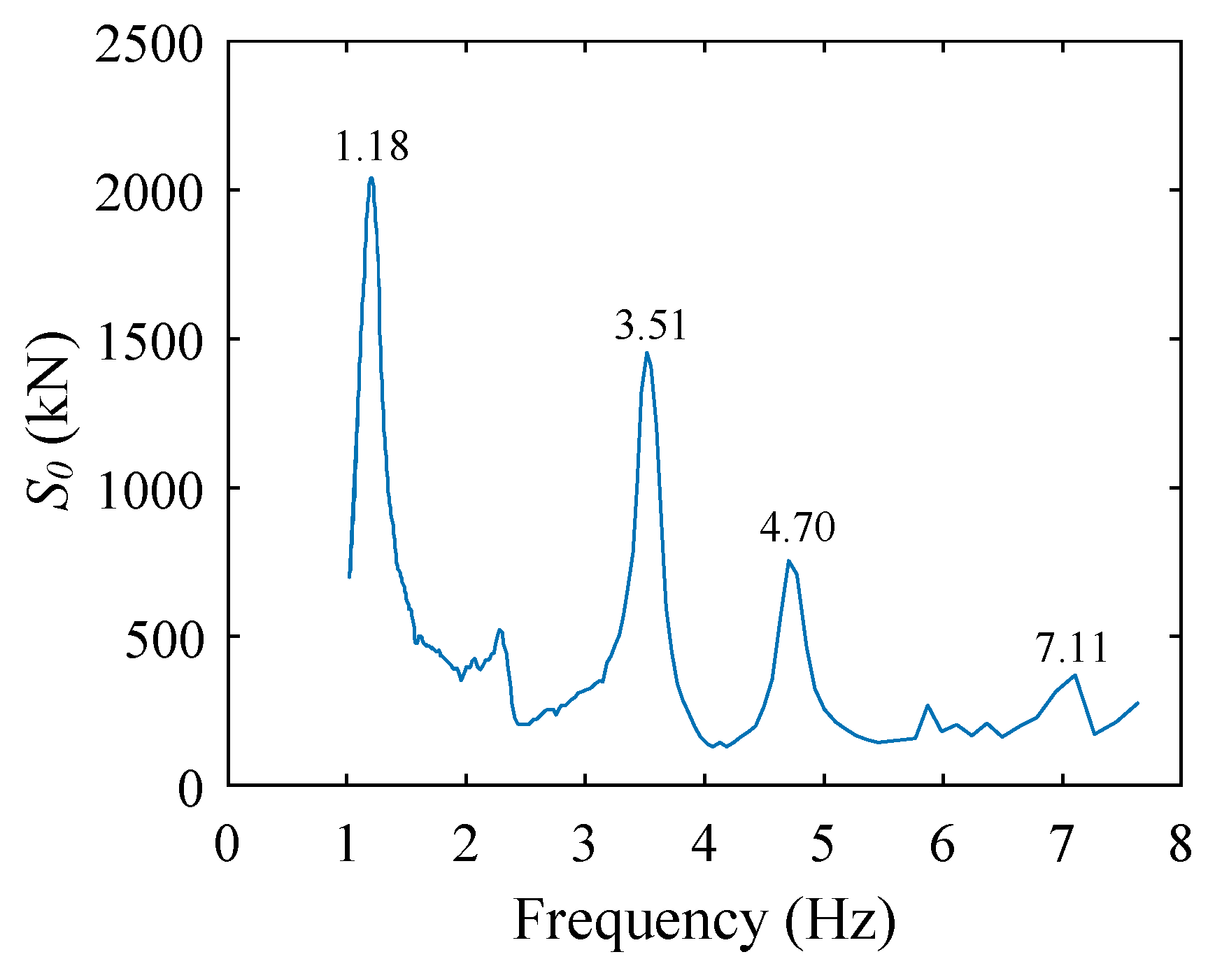
The validation has been performed by comparing the vertical acceleration measurements obtained in the tests under railway traffic with the corresponding numerical results obtained with the train-bridge interaction tool described in Section 2.3. The experimental measurements used in the validation process correspond to those obtained with the accelerometers no. 3 (opposite track) and no. 4 (running track) shown in Figure 12 due to the passage of the Alfa Pendular train at 110 km/h in the Porto-Lisbon direction. Figure 21 depicts the train signature of the Alfa Pendular, highlighting the main frequencies associated with the passage of axles or group of axles. The train signature is an important tool to understand the dynamic response of the bridge subjected to railway traffic, as will be referred in the following sections. All the results, both numerical and experimental, were filtered using a Chebyshev Type II low-pass digital filter of order 8, a stopband attenuation equal to 45 dB and a cut-off frequency of 30 Hz.
The dynamic analyses have been performed considering a timestep Δt of 0.001 s and an α parameter equal to 0, which corresponds to the Newmark method (β = 0.25 and γ = 0.5). Regarding damping, the mean value ξ ¯ = 6.69 % estimated with the Prony method for different train passages has been adopted in the numerical model (see Section 3.2). However, since the governing equilibrium equations of motion are solved through a direct integration scheme, a Rayleigh damping matrix proportional to the mass and stiffness matrix [50] had to be considered in the analysis. The proportionality constants were obtained by setting the target damping of the structure in two frequencies fi and fj, guaranteeing that all the vibration modes within this interval become underdamped and the remaining ones outside it become overdamped. In this work, fi corresponds to the first identified vibration mode (fi = 10.10 Hz), while fj corresponds to the fourth one (fj = 35.58 Hz). Such consideration guarantees the correct representation of the damping coefficient of the main mode of the structure (first mode), while avoiding an overestimation of the damping in the following identified modes. In the frequency range between 10.10 Hz and 35.58 Hz, the dynamic response of the bridge is not influenced by the dynamic behaviour of the track. The track dynamics associated with the movements of the ballast layer, typically occurs in the frequency range between 80 Hz and 150 Hz [51]. Thus, for solving the train-track-bridge dynamic interaction problem the track behaves as a rigid layer, i.e., no relative movements between the rails and deck occur due to the track dynamic flexibility.
The track irregularities used in the dynamic analyses were recorded by the inspection vehicle EM120 from the Portuguese infrastructure manager one month before the dynamic tests. Figure 22 illustrates the longitudinal level irregularity profile on both rails between km +100.55 and +100.70 of the Northern line (Porto-Lisbon direction), including the location of the Cascalheira bridge.
This section presents the validation results based on different FE models of the Cascalheira bridge with increasing levels of agreement with the real structure. First, the comparison between experimental and numerical results obtained with the numerical model defined by the parameters adopted before and after the updating process is presented in Section 5.2. However, this updating has been performed based on the levels of acceleration obtained in the ambient vibration tests, which are significantly lower than those obtained in the tests under railway traffic. Therefore, two modifications have been carried out in the model to achieve a better agreement between numerical and experimental results. The first one, which is discussed in Section 5.3, consists of a reduction in the stiffness of the bearing supports to take into consideration a possible degradation scenario, as well as predictable non-linear behaviour of these devices. Then, a second modification that takes into consideration the degradation of the ballast over the longitudinal joint due to the distortions that occur in this region under traffic loads is also evaluated. This last scenario, presented in Section 5.4, is simulated through a decrease in the modulus of elasticity of the ballast, which has been evaluated based on the shear strains observed in the joint between the two half-decks and computed with the numerical model.
Finally, to complement the visual comparison between experimental and numerical results, an indicator proposed by Sarin et al. [52], called normalized Mean Absolute Error (nMAE), has also been used to evaluate the quality of the match between the two time-histories. This indicator makes use of the Dynamic Time Warping (DTW) technique, which compensates the time shifts that may exist between numerical and experimental records due to vehicle’s speed variations. Mathematically, the nMAE indicator may be defined as
nMAE = N E 1 E 1
where N E 1 is the L1 norm between the vectors containing numerical (N) results and experimental (E) data and E 1   is the L1 norm of the experimental data.

5.2. Comparison between Numerical and Experimental Bridge Response before and after the Updating Process

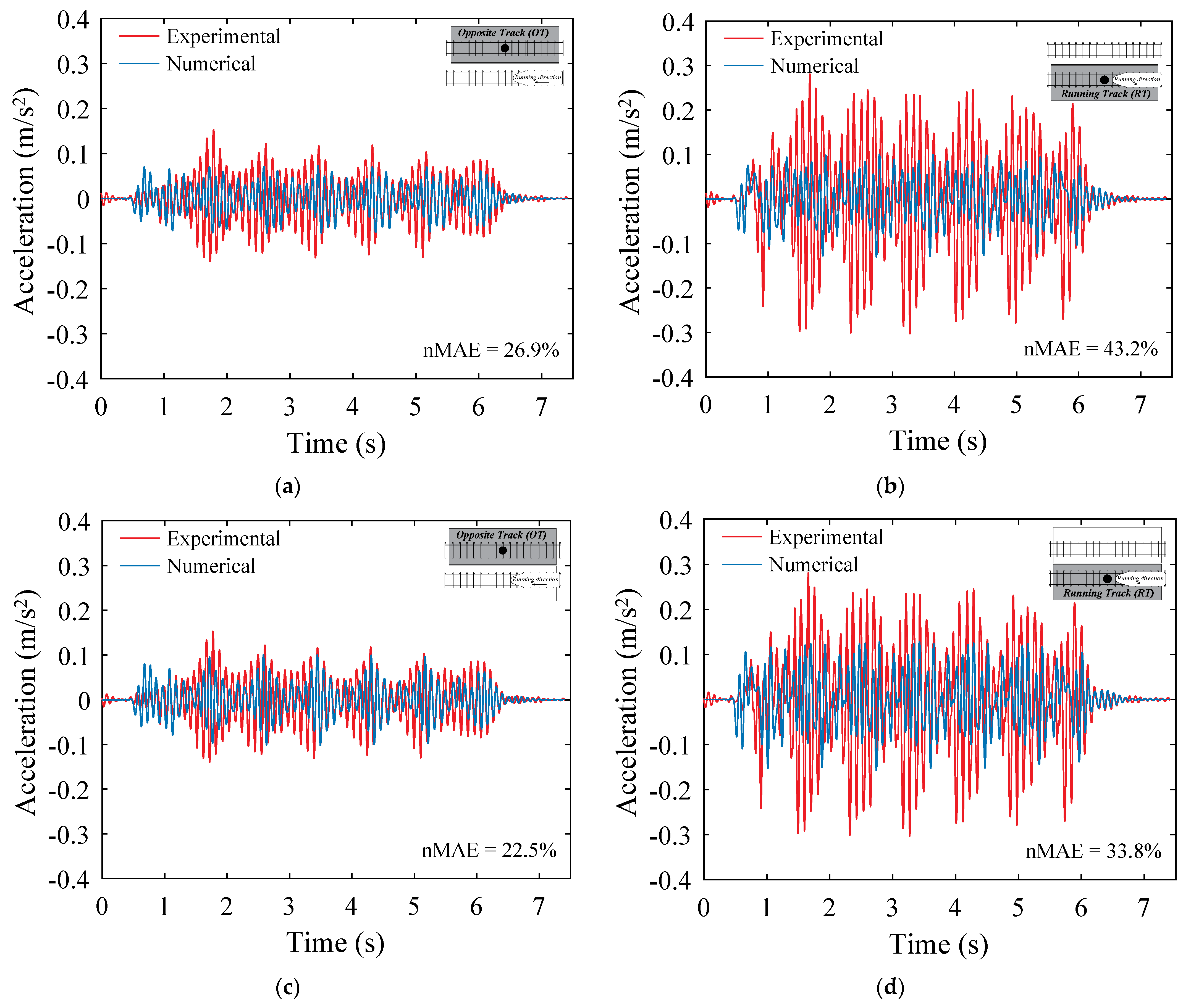
Figure 23 presents the comparison between the experimental accelerations measured by the sensors installed at the midspan in the opposite (OT) and running tracks (RT) with the corresponding numerical results obtained with the bridge model before and after updating. By looking to the results, a good match between the experimental and numerical response shapes can be observed on both locations. However, the agreement is not so satisfactory in terms of amplitude in the model before updating, especially in the running track side. In terms of the nMAE indicator obtained with this model, it takes the values of 26.9% and 43.2% in the results regarding the OT and RT, respectively, which is still considerably high.
When comparing the results obtained with the model developed before and after the updating process, a better agreement between numerical and experimental results can be observed on both tracks with the latter model. This improvement, which is especially notorious in the RT track, can be observed not only by visually comparing the time-histories but also by analysing the nMAE indicator, since it decreases to 22.5% and 33.8% in the OT and RT sides, respectively.
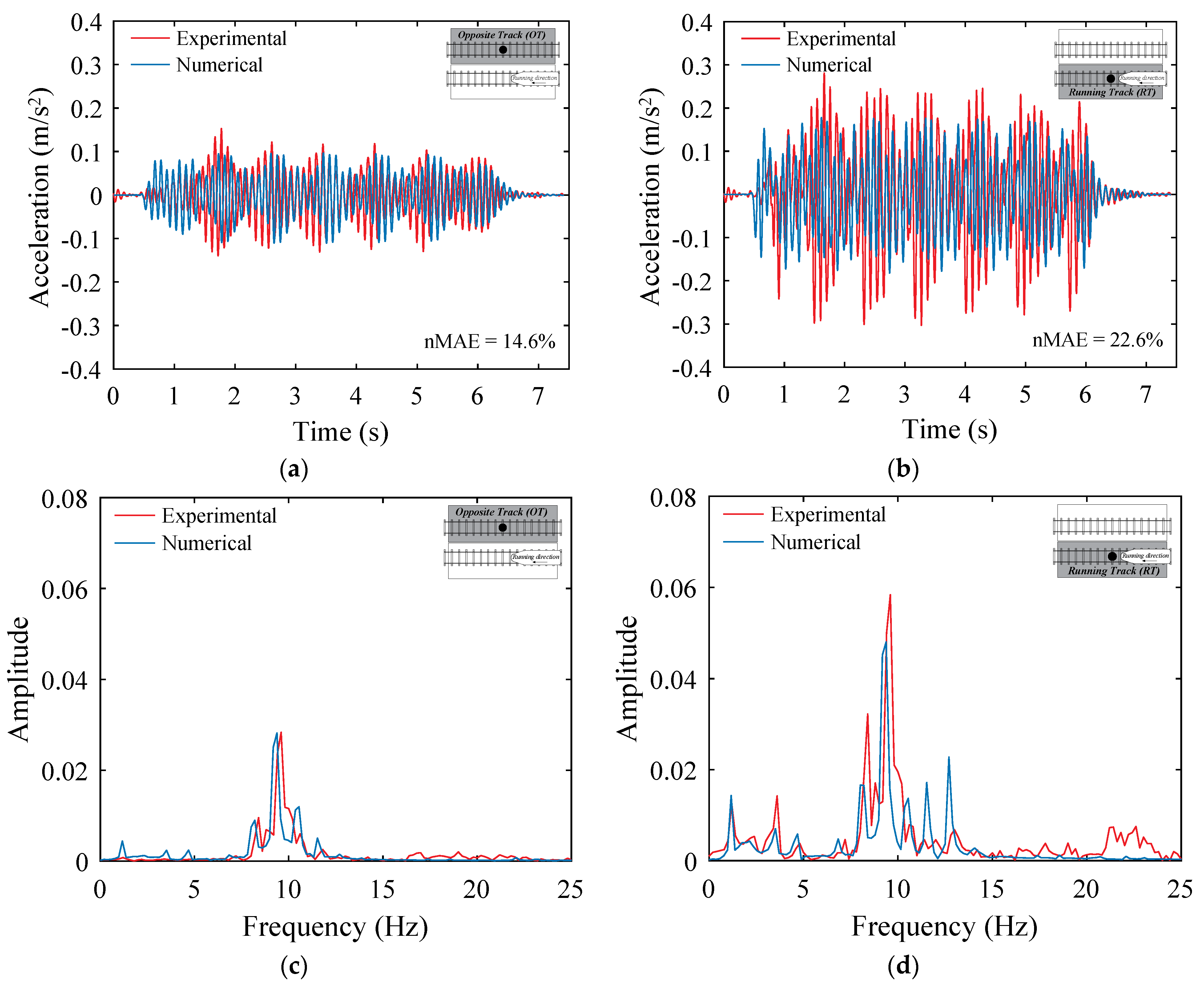
By analysing the frequency content of the responses obtained after the updating process and depicted in Figure 24, it is possible to observe that the first peaks are associated with the passage of the axles and groups of axles of the train, in accordance with the train signature presented before in Figure 21, while the highest peaks, around 10 Hz, are associated with the first vibration mode of the bridge. A relatively good agreement in terms of the frequency of the peaks is observed, whereas the amplitude remains relatively different even after updating. It is important to note, however, that the updating of the numerical model described in Section 4 was based on modal properties obtained through the acceleration records obtained in ambient vibration tests, while this validation is caried out using acceleration responses with much higher amplitude recorded in tests under railway traffic. Hence, to obtain a closer match between experimental and numerical data, two modifications have been made in the calibrated model, more specifically in the vertical stiffness of the bearing supports and in the modulus of elasticity of the ballast from the longitudinal joint. The influence of these two factors is discussed in the following sections.

5.3. Influence of the Vertical Stiffness of the Bearing Supports

The first modification in the numerical model considered in the present validation was related with the evaluation of the influence of the vertical stiffness of the bearing supports in the acceleration response of the deck. The model updating led to a stiffness Kv equal to 194.9 MN/m, which is close to the original lower bound adopted in the updating process. However, it was noticed that the numerical acceleration responses calculated on both tracks tend to match the corresponding experimental ones for lower levels of stiffness, which can be justified by a degradation of the elastomeric material present in the bearing supports, as well as by a reduction in the confinement provided by the steel sheets or by the possible non-linear behaviour of these devices. Based on this assumption, a modified model was obtained through a successive reduction in the vertical stiffness of the supports until reaching the value of 132 MN/m, which guaranteed the best compromise in terms of agreement between the numerical and experimental accelerations on both track sides. Figure 25 compares the numerical midspan accelerations obtained in the opposite (OT) and running tracks (RT) with those recorded experimentally by the accelerometers installed at these locations. A significant improvement in the agreement between the results is notorious, showing that the numerical model with the proposed modification captures with more accuracy the actual behaviour of the bridge. This conclusion is evident not only by observing the responses, but also by looking into the nMAE indicator, which decreased to 14.6% (22.5% in the previous model) and 22.6% (33.8% in the previous model) with respect to the results obtained in the OT and RT, respectively. Finally, in the frequency domain, a better match between the amplitudes of the peaks has also been achieved, especially in the main peak related with the first mode of vibration of the bridge around 10 Hz.

5.4. Influence of the Degradation of the Longitudinal Joint

The Cascalheira bridge is composed by two half-decks separated by a longitudinal joint. Although structurally separated, these half-decks are slightly connected through the track continuity effect provided by the ballast. The updating process led to a significant decrease in the modulus of elasticity of the ballast over the longitudinal joint Eb2, from 145 MPa to 76.25 MPa (see Figure 18), which demonstrates a possible degradation of the ballast over this region. However, this degradation tends to be more pronounced with the shear strain levels (distortion) that may occur in these joints due to the relative cyclic movements between adjacent half-decks caused by the train passages. These effects, which have been reported in the literature [8,53], may lead to modifications in the structural response. Hence, based on the numerically evaluated distortions of the ballast at the joint level, the degradation of the elasticity modulus of the ballast has been estimated to evaluate if it may influence the correspondence between numerical and experimental data.
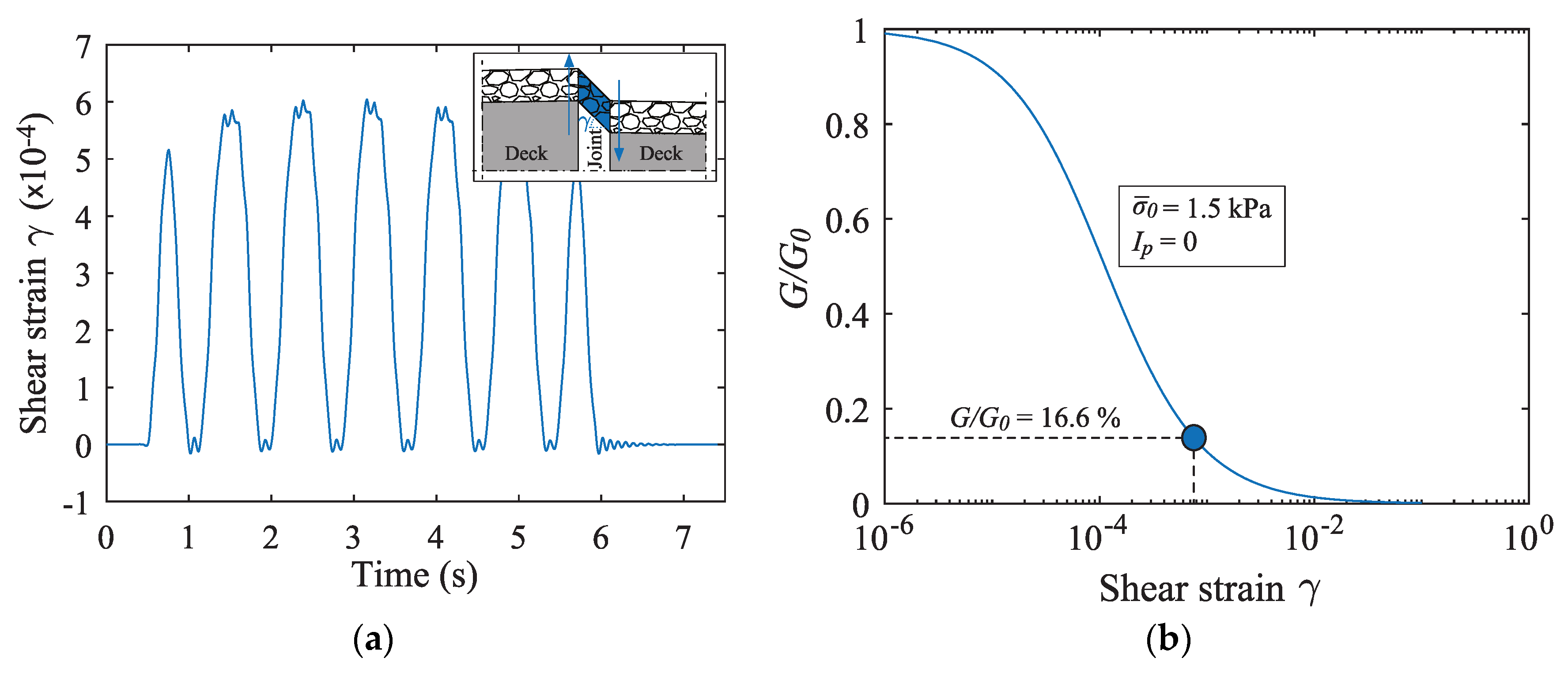
The cyclic shear strains γ in the longitudinal joint, evaluated at the midspan of the bridge due to the passage of the Alfa Pendular train at 110 km/h and computed with the numerical model presented in the previous section, are plotted in Figure 26a. To evaluate the level of degradation of the ballast over the joint due to the cyclic shear strain, a shear modulus degradation curve G / G 0 ( γ ) proposed by Ishibashi et al. [30] has been adopted and is represented in Figure 26b. According to the authors, this curve, which represents the ratio between the shear modulus G of the material subjected to a shear strain γ and the initial shear modulus of the same material without being subjected to any distortion, G0, can be mathematically described by:
G G 0 ( γ ) = K ( γ , I p ) σ ¯ 0 m ( γ , I p ) m 0
where σ ¯ 0 is the mean effective confining pressure and K ( γ , I p ) and m ( γ , I p ) m 0 are factors that depend on the shear strain γ and plasticity index Ip (see Ishibashi et al. [30] for details regarding the curve equation). Given the nature of the ballast material, a small confining pressure of 1.5 kPa and a null plasticity index (PI) has been adopted to trace the degradation curve presented in Figure 26b. The results show that the maximum level of shear strain due to the train passage is equal to 6.04 × 10 4 , which corresponds to a degradation of 16.6% of the shear (and elasticity modulus of the ballast over the joint). Therefore, it is acceptable to consider reductions of Eb2 in this order of magnitude in the numerical model (16.6% of 76.25 MPa equal to 12.66 MPa).
After performing successive reductions in this parameter within the lower bound obtained in the distortion analysis (Eb2 = 12.66 MPa), an optimal value of 36 MPa has been obtained, which guaranteed a compromise in the agreement between the numerical and experimental data on both track sides. Figure 27 depicts the midspan numerical and experimental acceleration results relative to both the opposite (OT) and running tracks (RT) in the time and frequency domains. Note that, by degrading the longitudinal joint, the continuity between both half-decks decreases, leading to a slight decrease in the accelerations in the OT side and an increase in the RT side. The effect caused by this modification led to the lowest values of the nMAE indicator on both OT and RT sides, which took the values of 13.4% to 21.1%, respectively. In the frequency domain, the enhancements made in the numerical model described in Section 5.3 and Section 5.4 also led to notorious improvements, since the errors in the main peak’s amplitude related with the bridge’s first mode of vibration decreased from 46% and 54% in the OT and RT sides, respectively, to just 11% and 8%.

6. Conclusions

The present paper aimed to develop, calibrate and validate a numerical model of a filler beam type double-deck bridge under operational conditions. The study starts with the development of the FE model of the bridge-track system, followed by its updating with a genetic algorithm based on modal experimental data. Finally, the validation of the model is carried out through the comparison between the experimental responses of the bridge acquired with accelerometers located on the two half-decks with those computed numerically with a train-bridge interaction dynamic tool. Therefore, based on the obtained results, the following conclusions can be drawn:
  • The ambient vibration test allowed the identification of four global modes, namely the first and second vertical bending modes and two torsion modes. These modes were also identified in the initial numerical model, although still with considerable differences in terms of frequency value (errors up to almost 5%).
  • Experimental modal damping was identified using the free vibration records obtained in the tests under railway traffic. Given the difficulty in separating the contribution of the first bending and torsional modes for the free vibration (frequencies close to each other), the Prony method was used. By adopting this methodology to the records obtained during the tests under railway traffic, mean damping ratios of 6.69% and 4.72% were estimated for the first bending and torsional modes, respectively.
  • Before performing the automatic optimization process, a sensitivity analysis was carried out, showing that 5 out of the 13 analysed parameters had a significant influence in the modal response, namely the modulus of elasticity of the concrete and ballast in the longitudinal joint, the density of concrete and ballast and the vertical stiffness of the bearing supports. Based on this outcome, an updating procedure based on a genetic algorithm was carried out to calibrate the numerical model. A significant reduction in the differences between numerical and experimental natural frequencies was achieved; more precisely, the average error of the frequencies decreased from 2.65% before updating, to 0.69% after updating. Regarding the MAC coefficients, they suffer an overall increase, reaching values close to 1.0 (between 0.968 and 0.997).
  • Regarding the validation of the model, a good agreement between experimental and numerical results was observed, in particular with the model obtained after the updating. The improvement in the results was confirmed through the nMAE indicator, which reduced from 26.9% to 22.5% and from 43.2% to 33.8% regarding the responses obtained in the OT and RT sides, respectively. However, as confirmed with the results in the frequency domain, the amplitudes of the numerical and experimental responses were still considerably different, especially in the RT side. Therefore, to improve the results, and since the updating process was based on modal data obtained with ambient vibration measurements, two modifications in the FE model of the bridge were carried out with the objective of getting a closer match between experimental and numerical responses of the bridge under railway traffic.
  • Since the vertical stiffness of the bearing supports proved to have a significant influence in the model updating process, an evaluation of its influence in the vertical response of the bridge was conducted. After performing successive changes to this parameter, a vertica1 stiffness of 132 MN/m was achieved, which guaranteed a compromise in terms of agreement between the numerical and experimental accelerations on both track sides. By doing so, the numerical time-histories significantly approached the experimental ones and the nMAE indicator suffered a significant reduction to 14.6% and 22.6% relative to the responses obtained in OT and RT sides, respectively. This enhancement was also notable in the frequency domain, since the amplitudes of the main peaks obtained in the numerical analyses increased, showing a better agreement with the measured data.
  • Finally, the behaviour of the ballast located over the longitudinal joint was also analysed. The effects of a possible degradation of this material were evaluated based on the shear strain levels that occur in the joint due to the relative cyclic movements between the two adjacent half-decks. After evaluating the maximum plausible degradation of the ballast layer over the joint through a shear modulus degradation curve, a reduction in the modulus of elasticity of the ballast on this location was tested. An optimal value of 36 MPa was obtained, which guaranteed the best compromise in the agreement between numerical and experimental results. By doing so, the numerical results improved in relation to the experimental ones, leading to the lowest levels of the nMAE indicator on both sides, more specifically 13.4% to 21.1% with respect to the OT and RT sides, respectively.
The present work demonstrated that a proper updating and validation of the numerical model can significantly improve its capabilities for reproducing the effects caused by the passage of trains.

Author Contributions

Conceptualization, P.A.M. and D.R.; Formal analysis, S.S.; Funding acquisition, R.C.; Investigation, G.S. and A.S.; Methodology, P.A.M. and D.R.; Project administration, R.C.; Software, P.A.M.; Supervision, S.S. and R.C.; Validation, D.R.; Visualization, P.A.M.; Writing—original draft, G.S. and A.S.; Writing—review & editing, P.A.M., D.R. and R.C. All authors have read and agreed to the published version of the manuscript.

Funding

This work has been supported by the projects IN2TRACK2 and IN2TRACK3 funded by the Shift2Rail Joint Undertaking under the European Union’s Horizon 2020 research and innovation programme under grant agreements No. 826255 and No. 101012456, respectively. Moreover, this work was also financially supported by Base Funding—UIDB/04708/2020 and Programmatic Funding—UIDP/04708/2020 of the CONSTRUCT—Instituto de I&D em Estruturas e Construções—funded by national funds through the FCT/MCTES (PIDDAC). Finally, the second and fourth authors acknowledge Grant No. 2020.00305.CEECIND from the Stimulus of Scientific Employment, Individual Support (CEECIND)—3rd Edition provided by “FCT—Fundação para a Ciência e Tecnologia” and project operation NORTE-08-5369-FSE-000027 by Norte Portugal Regional Operational Programme (NORTE 2020), under the PORTUGAL 2020 Partnership Agreement, through the European Social Fund (ESF), respectively.

Conflicts of Interest

The authors declare no conflict of interest.

References

  1. Zhai, W.; Cai, C. Effect of Locomotive Vibrations on Pantograph-Catenary System Dynamics. Veh. Syst. Dyn. 1998, 29, 47–58. [Google Scholar] [CrossRef]
  2. Song, Y.; Wang, Z.; Liu, Z.; Wang, R. A spatial coupling model to study dynamic performance of pantograph-catenary with vehicle-track excitation. Mech. Syst. Signal Process. 2020, 151, 107336. [Google Scholar] [CrossRef]
  3. Galvín, P.; Romero, A.; Moliner, E.; De Roeck, G.; Martínez-Rodrigo, M. On the dynamic characterisation of railway bridges through experimental testing. Eng. Struct. 2020, 226, 111261. [Google Scholar] [CrossRef]
  4. Montenegro, P.; Carvalho, H.; Ribeiro, D.; Calçada, R.; Tokunaga, M.; Tanabe, M.; Zhai, W. Assessment of train running safety on bridges: A literature review. Eng. Struct. 2021, 241, 112425. [Google Scholar] [CrossRef]
  5. Olmos, J.; Astiz, M. Improvement of the lateral dynamic response of a high pier viaduct under turbulent wind during the high-speed train travel. Eng. Struct. 2018, 165, 368–385. [Google Scholar] [CrossRef]
  6. Meixedo, A.; Ribeiro, D.; Calçada, R.; Delgado, R. Global and Local Dynamic Effects on a Railway Viaduct with Precast Deck. Engineering 2014, 104, 77. [Google Scholar] [CrossRef]
  7. Zangeneh, A.; Svedholm, C.; Andersson, A.; Pacoste, C.; Karoumi, R. Identification of soil-structure interaction effect in a portal frame railway bridge through full-scale dynamic testing. Eng. Struct. 2018, 159, 299–309. [Google Scholar] [CrossRef]
  8. Melo, L.R.T.; Ribeiro, D.; Calçada, R.; Bittencourt, T.N. Validation of a vertical train–track–bridge dynamic interaction model based on limited experimental data. Struct. Infrastruct. Eng. 2019, 16, 181–201. [Google Scholar] [CrossRef]
  9. Zhai, W.; Han, Z.; Chen, Z.; Ling, L.; Zhu, S. Train-track-bridge dynamic interaction: A state-of-the-art review. Veh. Syst. Dyn. 2019, 57, 984–1027. [Google Scholar] [CrossRef] [Green Version]
  10. He, X.; Gai, Y.; Wu, T. Simulation of train–bridge interaction under wind loads: A rigid-flexible coupling approach. Int. J. Rail Transp. 2017, 6, 163–182. [Google Scholar] [CrossRef]
  11. Antolín, P.; Zhang, N.; Goicolea, J.M.; Xia, H.; Astiz, M.; Oliva, J. Consideration of nonlinear wheel–rail contact forces for dynamic vehicle–bridge interaction in high-speed railways. J. Sound Vib. 2013, 332, 1231–1251. [Google Scholar] [CrossRef]
  12. Zhang, N.; Xia, H. Dynamic analysis of coupled vehicle–bridge system based on inter-system iteration method. Comput. Struct. 2013, 114–115, 26–34. [Google Scholar] [CrossRef]
  13. Szafrański, M. A dynamic vehicle-bridge model based on the modal identification results of an existing EN57 train and bridge spans with non-ballasted tracks. Mech. Syst. Signal Process. 2020, 146, 107039. [Google Scholar] [CrossRef]
  14. Ribeiro, D.; Calçada, R.; Delgado, R.; Brehm, M.; Zabel, V. Finite-element model calibration of a railway vehicle based on experimental modal parameters. Veh. Syst. Dyn. 2013, 51, 821–856. [Google Scholar] [CrossRef]
  15. Tomioka, T.; Takigami, T.; Suzuki, Y. Numerical analysis of three-dimensional flexural vibration of railway vehicle car body. Veh. Syst. Dyn. 2006, 44, 272–285. [Google Scholar] [CrossRef]
  16. Chellini, G.; Nardini, L.; Salvatore, W. Dynamical identification and modelling of steel–concrete composite high-speed railway bridges. Struct. Infrastruct. Eng. 2011, 7, 823–841. [Google Scholar] [CrossRef]
  17. Axelsson, E.; Syk, A.; Ülker-Kaustell, M.; Battini, J.-M. Effect of Axle Load Spreading and Support Stiffness on the Dynamic Response of Short Span Railway Bridges. Struct. Eng. Int. 2014, 24, 457–465. [Google Scholar] [CrossRef] [Green Version]
  18. Museros, P.; Romero, M.; Poy, A.; Alarcón, E. Advances in the analysis of short span railway bridges for high-speed lines. Comput. Struct. 2002, 80, 2121–2132. [Google Scholar] [CrossRef] [Green Version]
  19. Bornet, L.; Andersson, A.; Zwolski, J.; Battini, J.-M. Influence of the ballasted track on the dynamic properties of a truss railway bridge. Struct. Infrastruct. Eng. 2014, 11, 796–803. [Google Scholar] [CrossRef]
  20. Melo, L.R.T.; Malveiro, J.; Ribeiro, D.; Calçada, R.; Bittencourt, T. Dynamic analysis of the train-bridge system considering the non-linear behaviour of the track-deck interface. Eng. Struct. 2020, 220, 110980. [Google Scholar] [CrossRef]
  21. Rauert, T.; Bigelow, H.; Hoffmeister, B.; Feldmann, M. On the prediction of the interaction effect caused by continuous ballast on filler beam railway bridges by experimentally supported numerical studies. Eng. Struct. 2010, 32, 3981–3988. [Google Scholar] [CrossRef]
  22. Sánchez-Quesada, J.; Moliner, E.; Romero, A.; Galvín, P.; Martínez-Rodrigo, M. Ballasted track interaction effects in railway bridges with simply-supported spans composed by adjacent twin single-track decks. Eng. Struct. 2021, 247, 113062. [Google Scholar] [CrossRef]
  23. Stollwitzer, A.; Fink, J.; Malik, T. Experimental analysis of damping mechanisms in ballasted track on single-track railway bridges. Eng. Struct. 2020, 220, 110982. [Google Scholar] [CrossRef]
  24. Battini, J.-M.; Ülker-Kaustell, M. A simple finite element to consider the non-linear influence of the ballast on vibrations of railway bridges. Eng. Struct. 2011, 33, 2597–2602. [Google Scholar] [CrossRef]
  25. Rebelo, C.; Simoesdasilva, L.; Rigueiro, C.; Pircher, M. Dynamic behaviour of twin single-span ballasted railway viaducts—Field measurements and modal identification. Eng. Struct. 2008, 30, 2460–2469. [Google Scholar] [CrossRef]
  26. Rigueiro, C.; Rebelo, C.; Simoesdasilva, L. Influence of ballast models in the dynamic response of railway viaducts. J. Sound Vib. 2010, 329, 3030–3040. [Google Scholar] [CrossRef]
  27. Malveiro, J.; Ribeiro, D.; Sousa, C.; Calçada, R. Model updating of a dynamic model of a composite steel-concrete railway viaduct based on experimental tests. Eng. Struct. 2018, 164, 40–52. [Google Scholar] [CrossRef]
  28. Brehm, M.; Zabel, V.; Bucher, C. An automatic mode pairing strategy using an enhanced modal assurance criterion based on modal strain energies. J. Sound Vib. 2010, 329, 5375–5392. [Google Scholar] [CrossRef]
  29. Zhai, W.; Wang, S.; Zhang, N.; Gao, M.; Xia, H.; Cai, C.; Zhao, C. High-speed train–track–bridge dynamic interactions—Part II: Experimental validation and engineering application. Int. J. Rail Transp. 2013, 1, 25–41. [Google Scholar] [CrossRef]
  30. Ishibashi, I.; Zhang, X. Unified Dynamic Shear Moduli and Damping Ratios of Sand and Clay. Soils Found. 1993, 33, 182–191. [Google Scholar] [CrossRef] [Green Version]
  31. ERRI. Railway Bridges for Speeds >200 km/h, Recommendations for Calculating Damping in Rail Bridge Decks; European Rail Research Institute: Utrecht, The Netherlands, 1999. [Google Scholar]
  32. ANSYS®. 2018. Available online: https://www.ansys.com/ (accessed on 28 March 2022).
  33. Manterola, J. Puentes: Apuntes Para su Diseño, Cálculo y Construcción; Colegio de Ingenieros de Caminos, Canales y Puertos: Madrid, Spain, 2006. [Google Scholar]
  34. Henriques, A.A.R. Aplicação de Novos Conceitos de Segurança No Dimensionamento do Betão Estrutural; University of Porto: Porto, Portugal, 1998. [Google Scholar]
  35. Neville, A.M. Properties of Concrete, 4th ed.; John Wiley and Sons: New York, NY, USA, 1996. [Google Scholar]
  36. Ricci, L.; Nguyen, V.; Sab, K.; Duhamel, D.; Schmitt, L. Dynamic behaviour of ballasted railway tracks: A discrete/continuous approach. Comput. Struct. 2005, 83, 2282–2292. [Google Scholar] [CrossRef]
  37. Shahu, J.T.; Rao, N.K. Yudhbir Parametric study of resilient response of tracks with a sub-ballast layer. Can. Geotech. J. 1999, 36, 1137–1150. [Google Scholar] [CrossRef]
  38. Montenegro, P.A. A Methodology for the Assessment of the Train Running Safety on Bridges. Ph.D. Thesis, Faculty of Engineering of the University of Porto, Porto, Portugal, 2015. [Google Scholar]
  39. Ribeiro, D. Dynamic Effects Induced by Traffic in Railway Bridges: Numerical Modeling, Calibration and Experimental Validation. Ph.D. Thesis, Faculty of Engineering of the University of Porto, Porto, Portugal, 2012. (In Portuguese). [Google Scholar]
  40. Montenegro, P.A.; Neves, S.; Calçada, R.; Tanabe, M.; Sogabe, M. Wheel–rail contact formulation for analyzing the lateral train–structure dynamic interaction. Comput. Struct. 2015, 152, 200–214. [Google Scholar] [CrossRef] [Green Version]
  41. Hertz, H. Ueber die Berührung fester elastischer Körper. Mathematik 1882, 1882, 156–171. [Google Scholar] [CrossRef]
  42. Shabana, A.A.; Zaazaa, K.E.; Sugiyama, H. Railroad Vehicle Dynamics: A computational Approach; CRC Press—Taylor & Francis Group: Boca Raton, FL, USA, 2008. [Google Scholar]
  43. Kalker, J. Book of tables for the Hertzian creep-force law. In Proceedings of the 2nd Mini Conference on Contact Mechanics and Wear of Wheel/Rail Systems, Budapest, Hungary, 29–31 July 1996. [Google Scholar]
  44. Hughes, T.J.R. The Finite Element Method: Linear Static and Dynamic Finite Element Analysis; Dover Publications: New York, NY, USA, 2000. [Google Scholar]
  45. MATLAB®. 2020. Available online: https://www.mathworks.com/products/matlab.html (accessed on 28 March 2022).
  46. ARTeMIS. ARTeMIS Extractor Pro—Academic License, User’s Manual, SVS 2009; ARTeMIS: Eindhoven, The Netherlands, 2009. [Google Scholar]
  47. Marple, S.L. Digital Spectral Analysis: Second Edition; Courier Dover Publications: New York, NY, USA, 2019. [Google Scholar]
  48. Petsounis, K.; Fassois, S. Parametric Time-Domain Methods for The Identification of Vibrating Structures—A Critical Comparison and Assessment. Mech. Syst. Signal Process. 2001, 15, 1031–1060. [Google Scholar] [CrossRef]
  49. Allemang, R.J. The modal assurance criterion–twenty years of use and abuse. Sound Vib. 2003, 37, 14–23. [Google Scholar]
  50. Clough, R.W.; Penzien, J. Dynamic of Structures, 3rd ed.; McGraw-Hill, Inc.: New York, NY, USA, 2003. [Google Scholar]
  51. Ribeiro, D.; Calçada, R.; Brehm, M.; Zabel, V. Calibration of the numerical model of a track section over a railway bridge based on dynamic tests. Structures 2021, 34, 4124–4141. [Google Scholar] [CrossRef]
  52. Sarin, H.; Kokkolaras, M.; Hulbert, G.; Papalambros, P.; Barbat, S.; Yang, R.-J. A Comprehensive Metric for Comparing Time Histories in Validation of Simulation Models with Emphasis on Vehicle Safety Applications. In Proceedings of the 2008 ASME International Design Engineering Technical Conferences and Computers and Information in Engineering Conference (DETC 2008), New York, NY, USA, 3–6 August 2008; pp. 1275–1286. [Google Scholar] [CrossRef] [Green Version]
  53. Liu, K.; Lombaert, G.; De Roeck, G. Dynamic Analysis of Multispan Viaducts with Weak Coupling between Adjacent Spans. J. Bridg. Eng. 2014, 19, 83–90. [Google Scholar] [CrossRef]
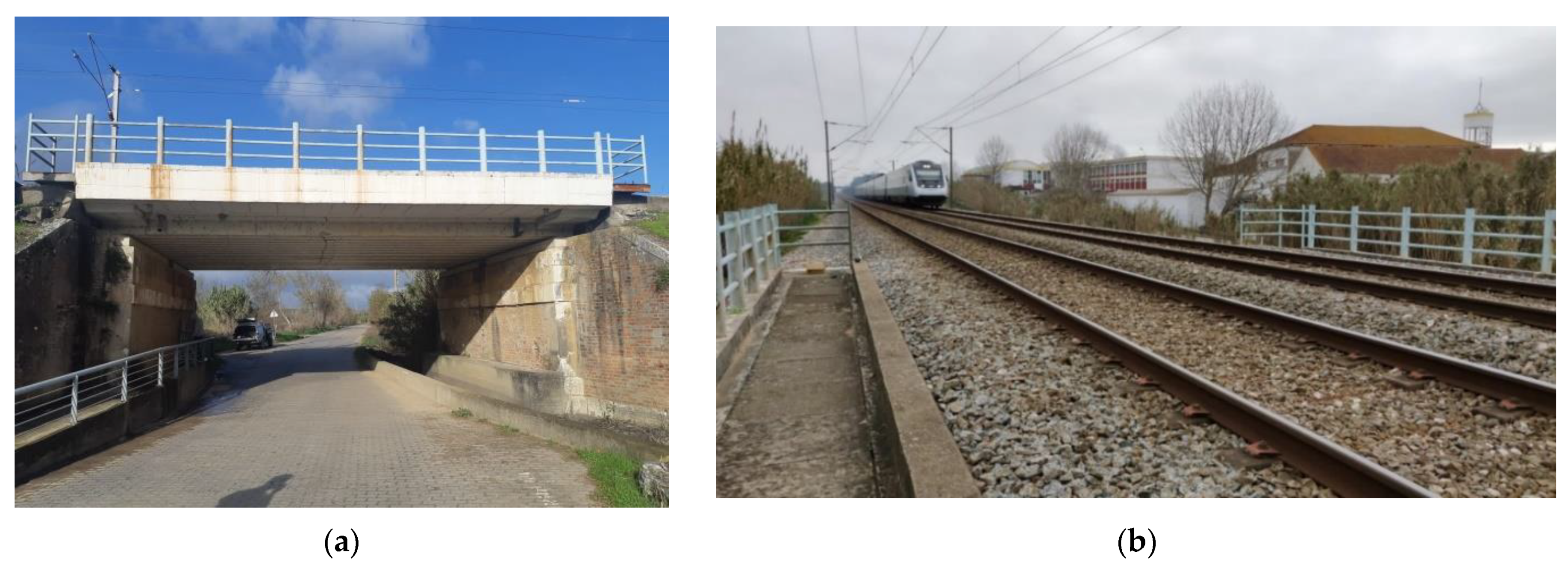
Figure 1. Cascalheira bridge: (a) global view; (b) track view; (c) cross-section (dimensions in cm).
Sustainability 14 05794 g001aSustainability 14 05794 g001b
Figure 2. Numerical model of the Cascalheira bridge.
Sustainability 14 05794 g002
Figure 3. Numerical modal parameters before updating.
Sustainability 14 05794 g003
Figure 4. Loading scheme of the Alfa Pendular train [14] (loads in kN).
Sustainability 14 05794 g004
Figure 5. Dynamic model scheme of a Alfa Pendular’s car (adapted from [38]): (a) transversal view and (b) lateral view.
Sustainability 14 05794 g005
Figure 6. Numerical model of the Alfa Pendular train.
Sustainability 14 05794 g006
Figure 7. Potential scenarios that arise from a valid solution of the nonlinear equations for contact search: (a) actual contact and (b) no contact.
Sustainability 14 05794 g007
Figure 8. Train-bridge interaction analysis performed with the VSI numerical tool.
Sustainability 14 05794 g008
Figure 9. Ambient vibration test: experimental setup including details of the accelerometer PCB 393B12 (dimensions in m).
Sustainability 14 05794 g009
Figure 10. EFDD method: Average normalized singular values of the spectral density matrices.
Sustainability 14 05794 g010
Figure 11. Experimental modal parameters.
Sustainability 14 05794 g011
Figure 12. Test under railway traffic: experimental setup including a detail of the accelerometer PCB 393A03 and highlighting the accelerometers located at midspan used to estimate damping (dimensions in m).
Sustainability 14 05794 g012
Figure 13. Location of the emitter and receiver optical sensors.
Sustainability 14 05794 g013
Figure 14. Methodology for the estimation of the damping coefficients based on the Prony method.
Sustainability 14 05794 g014
Figure 15. MAC matrix between numerical and experimental modes.
Sustainability 14 05794 g015
Figure 16. Spearman’s correlation matrix between the numerical parameters and modal responses.
Sustainability 14 05794 g016
Figure 17. Flowchart of the optimization strategy based on a genetic algorithm.
Sustainability 14 05794 g017
Figure 18. Values and ratio of the numerical parameters for optimization runs GA1 to GA4.
Sustainability 14 05794 g018
Figure 19. Correlation analysis between experimental and numerical modal parameters, before and after updating: (a) errors of natural frequencies; (b) MAC values.
Sustainability 14 05794 g019
Figure 20. Comparison between experimental and numerical mode shapes after updating.
Sustainability 14 05794 g020
Figure 21. Dynamic train signature of the Alfa Pendular for a running speed of 110 km/h.
Sustainability 14 05794 g021
Figure 22. Longitudinal level profile of irregularities used in the dynamic analyses.
Sustainability 14 05794 g022
Figure 23. Comparison between experimental and numerical vertical accelerations time-histories: (a) OT and (b) RT before updating; (c) OT and (d) RT after updating.
Sustainability 14 05794 g023
Figure 24. Comparison between experimental and numerical vertical accelerations in the frequency domain: (a) OT and (b) RT after updating.
Sustainability 14 05794 g024
Figure 25. Comparison between experimental and numerical vertical accelerations after updating and considering a modification in the vertical stiffness of the supports (Kv = 132 MN/m): (a) OT and (b) RT in the time domain; (c) OT and (d) RT in the frequency domain.
Sustainability 14 05794 g025
Figure 26. Effects in the longitudinal joint due to the train passage: (a) time-history of the shear strains and (b) shear modulus degradation for σ ¯ 0 = 1.5   kPa and PI = 0.
Sustainability 14 05794 g026
Figure 27. Comparison between experimental and numerical vertical accelerations after updating and considering a modification in the vertical stiffness of the supports (Kv = 132 MN/m) and in the modulus of elasticity of the ballast over the longitudinal joint (Eb2 = 36 MPa): (a) OT and (b) RT in the time domain; (c) OT and (d) RT in the frequency domain.
Sustainability 14 05794 g027
Table 1. Parameters of the numerical model of Cascalheira bridge.
ParametersStatistical PropertiesLimitsAdopted ValueReferences
Distribution TypeMean Value/Standard DeviationLowerUpper
Ec (GPa)Modulus of elasticity of concreteNormal37.4/3.7429.944.937.4[14,34,35]
ρc (kg/m3)Density of concreteNormal2500/250200030002500
υcPoisson ratio of concrete--/-0.160.240.20
Es (GPa)Modulus of elasticity of steelNormal210/8.4193.2226.8210.0[14]
ρs (kg/m3)Density of steel--/-770080007850
υsPoisson ratio of steel--/-0.280.320.30
Eb (MPa)Modulus of elasticity of ballastUniform169/22.5130208145[20,36,37]
Ebl (MPa)Modulus of elasticity of ballast (longitudinal joint)Uniform79.8/37.714.5145145
Ebt (MPa)Modulus of elasticity of ballast (transversal joints)Uniform79.8/37.714.5145145
ρb (kg/m3)Density of ballastUniform1800/260135022501800
υbPoisson ratio of ballast--/-0.150.200.15
Kv (MN/m)Vertical stiffness of the supportUniform355.5/111.7162549324[33]
Kh (kN/m)Horizontal stiffness of the supportUniform1730/47690525561809
Table 2. Parameters of the numerical model of the BBN vehicle (adapted from [39]).
ParametersUnitValue
Car bodyCar body massmcb (kg)38,445
Car body roll moment of inertiaIcb,x (kg·m2)55,120
Car body pitch moment of inertiaIcb,y (kg·m2)1,475,000
Car body yaw moment of inertiaIcb,z (kg·m2)1,477,000
BogieBogie massmb (kg)4858
Bogie roll moment of inertiaIb,x (kg·m2)2700
Bogie pitch moment of inertiaIb,y (kg·m2)1931.5
Bogie yaw moment of inertiaIb,z (kg·m2)3878.8
WheelsetWheelset massmw (kg)1711
Wheelset roll moment of inertiaIw,x (kg·m2)733.4
Wheelset yaw moment of inertiaIw,z (kg·m2)733.4
Primary suspensionStiffness of the primary longitudinal suspensionk1,x (N/m)4,498,100
Stiffness of the primary transversal suspension,k1,y (N/m)30,948,200
Stiffness of the primary vertical suspensionk1,z (N/m)1,652,820
Damping of the primary vertical suspensionc1,z (N·s/m)16,739
Secondary suspensionStiffness of the secondary longitudinal suspensionk2,x (N/m)4,905,000
Stiffness of the secondary transversal suspensionk2,y (N/m)2,500,000
Stiffness of the secondary vertical suspensionk2,z (N/m)734,832
Damping of the secondary longitudinal suspensionc2,x (N·s/m)400,000
Damping of the secondary transversal suspensionc2,y (N·s/m)17,500
Damping of the secondary vertical suspensionc2,z (N·s/m)35,000
Longitudinal distance between bogiesa1 (m)19
Longitudinal distance between wheelsetsa2 (m)2.7
Transversal distance between vertical secondary suspensionsb1 (m)2.144
Transversal distance between longitudinal secondary suspensionsb2 (m)2.846
Transversal distance between primary suspensionsb3 (m)2.144
Vertical distance between car body center and secondary suspensionh1 (m)0.936
Vertical distance between bogie center and secondary suspensionh2 (m)0.142
Vertical distance between bogie center and wheelset centerh3 (m)0.065
Nominal rolling radiusR0 (m)0.43
GaugeS (m)1.67
Table 3. Masses of the different vehicles belonging to the Alfa Pendular train.
VehicleCar Body (kg)Bogie [×2] (kg)Axle Average [×4] (kg)Total Sum (kg)
BAS36,9364858171153,496
BBS37,7524858171154,312
RNB35,9585204153852,518
RNH37,5485204153854,108
BBN38,4454858171155,005
BAN37,3454858171153,905
Table 4. Damping coefficients estimates based on the Prony method.
Train Speed (km/h)Mode 1Mode 2
f (Hz)amax (m/s2)ξ (%)f (Hz)amax (m/s2)ξ (%)
1109.210.07747.8611.930.02334.64
1359.570.09516.2011.460.18034.76
1409.550.07906.0111.560.18994.77
ξ ¯ = 6.69% ξ ¯ = 4.72%
Publisher’s Note: MDPI stays neutral with regard to jurisdictional claims in published maps and institutional affiliations.