Underwater Camera Calibration Method Based on Improved Slime Mold Algorithm

Abstract

The maritime transportation line is the lifeblood of the national economy. Transportation facilities and their construction equipment need to obtain the environmental parameters of relevant sea areas, and underwater robots are the first type of auxiliary equipment for underwater road construction. Considering that the construction of underwater transportation facilities puts forward higher requirements for the observation accuracy of underwater robots, the reliability of internal and external parameter calibration of underwater cameras directly affects the accuracy of underwater positioning and measurement. In order to improve the calibration accuracy of underwater cameras, this paper establishes a real underwater camera calibration image data set, integrates the optimal neighborhood disturbance and reverse learning strategy on the basis of the slime mold optimization algorithm, optimizes the calibration results of Zhang’s traditional calibration method, and compares the optimization results and reprojection error of the ORSMA algorithm with Zhang’s calibration method the SMA algorithm, SOA algorithm and PSO algorithm to verify the accuracy and effectiveness of the proposed algorithm.

1. Introduction

In recent years, with the rapid development of the cross-sea economy, the construction of the maritime transportation industry has also developed rapidly. Considering the complex and harsh working environments of underwater traffic construction, it is not suitable to use tools under ordinary working conditions, such as construction machinery for supervision and auxiliary operation of immersed tunnel construction, which means that underwater robots have gradually become one of the key tools for immersed tunnel construction. Compared with expensive underwater radars, cheap underwater cameras have become one of the main sensors of underwater robots. Therefore, whether the positioning and tracking of underwater targets can be accurately achieved, the precise calibration of the camera is particularly important. Accurate camera calibration is the premise of accurate positioning of underwater targets, and it is also one of the key technologies to promote the implementation of the strategy of strengthening the sea through science and technology.

As it is different from the calibration in the air, the changes in the underwater imaging model have an important impact on the camera calibration. Lavest J. M. et al. [1] considered both tangential and radial high-order distortions, transferred the corrected image to the air, and used the linear calibration method to calibrate the underwater camera, and obtained more accurate results. Agrawal et al. [2] established a multi-plane refraction underwater imaging model and proposed a camera calibration method based on the principle of coplanar constraints. The camera calibration method proposed by Anne Jordtsedlazeck [3] calibrates the camera’s internal parameters, external parameters and waterproof equipment parameters. This method is suitable for monocular and binocular calibration, but the process is complicated. Zhou [4] used the hidden point model to solve the iterative initial value of the camera’s internal parameters and proposed an improved version of Zhang’s calibration method that was applied to underwater scenes, which improved the accuracy of the iterative initial value. Zhang et al. [5] established a distortion correction model and corrected the camera parameters through the single-plane checkerboard camera calibration method.

With the gradual deepening of research, intelligent optimization algorithms are more and more applied in the field of camera calibration, which provides a new idea for improving calibration accuracy [6,7,8]. Research on more efficient algorithms has become a hot spot in the field of camera calibration. The existence of underwater environments and waterproof equipment makes the imaging process of underwater cameras very complicated, and the constructed underwater imaging model is very complicated and the solution process is very cumbersome [9]. However, the research time of the camera imaging model on land is longer, and the proposed model is also very mature. Therefore, it is a feasible way to introduce suitable intelligent optimization algorithms into the imaging model on land, so that the calibration parameters of the underwater camera can be solved. In this paper, a slime mold optimization algorithm (ORSMA), based on the fusion of the optimal neighborhood algorithm and reverse learning strategy, is proposed to optimize the process of solving camera parameters. The optimal neighborhood disturbance and reverse learning strategy are used to reduce the slime mold optimization. It is possible for the algorithm to fall into the local optimum, and the diversity of the population is maintained, and the convergence speed of the algorithm is improved to avoid the phenomenon of “prematurity”. The experimental results show that the algorithm proposed in this paper can effectively reduce the reprojection error of the camera, and the complexity of the algorithm is low, which provides a feasible optimization method for reducing the reprojection error of the camera.

2. Basic Principle of Slime Mold Optimization Algorithm

Slime mold algorithm (SMA) is a swarm intelligence algorithm proposed by Li et al. in 2020 [10]. SMA is a new stochastic optimizer and is proposed based upon the oscillation mode of slime molds in nature. The proposed SMA has several new features, with a unique mathematical model that uses adaptive weights to simulate the process of producing positive and negative feedback of the propagation wave of slime mold, based on bio-oscillators to form the optimal path for connecting food with excellent exploratory ability and exploitation propensity. The use of adaptive weights allows the SMA to maintain a certain perturbation rate while guaranteeing fast convergence, thus, avoiding local convergence during fast convergence. The SMA sets the vibration parameters, which allow individual locations of slime mold to contract in a specific way, thus, guaranteeing the efficiency of early exploration and the accuracy of late mining. The SMA has three different location update methods to ensure SMA adaptability at different search stages and it makes full use of individual fitness values to make better decisions. The results demonstrate that, compared with other meta-heuristic algorithms, the young slime mold algorithm has faster convergence ability and stronger optimization ability. The application of the slime mold algorithm in camera calibration can improve the efficiency and accuracy of calibration.

The results demonstrate that the algorithm proposed benefits from competitive, often outstanding, performance on different search landscapes.

Slime molds will oscillate and contract when they find food. At the same time, a vein network with different thickness will be formed between multiple food sources, and the thickness of the vein network is related to the quality of food sources. In addition, slime molds will still have a certain probability to search unknown areas when obtaining food sources. The main behaviors of slime molds are approaching food, wrapping food and obtaining food.

Slime molds can approach food according to the smell in the air. The higher the concentration of food in contact with the vein, the stronger the wave generated by the biological oscillator, the faster the flow of cytoplasm and the thicker the vein. The following mathematical formula can be used to simulate the update of the slime molds’ positions [10]:

$$\overrightarrow{X(t+1)}=\left\{\begin{array}{c}\overrightarrow{X_b(t)}+\overrightarrow{vb}\cdot (\overrightarrow{W}\cdot \overrightarrow{X_A(t)}-\overrightarrow{X_B(t)}),r<p\\ \overrightarrow{vc}\cdot \overrightarrow{X(t)},r\ge p\end{array}\right.$$

(1)

where $\overrightarrow{vb}$ is a parameter in the range $[a,-a]$, $\overrightarrow{vc}$ is a parameter linearly reduced from 1 to 0, t represents the current number of iterations, $\overrightarrow{X_b}$ represents the position of the individual with the highest fitness, $\overrightarrow{X}$ represents the position of the slime molds, $\overrightarrow{X_A}$ and $\overrightarrow{X_B}$ represent the positions of two randomly selected individuals in the slime molds and $\overrightarrow{W}$ represents the weight coefficient of the slime molds.

The expression formula of the control parameter p is as follows:

$$p=thnh|S(i)-DF|,i\in 1,2,3,\dots ,n$$

(2)

where $S(i)$ represents the fitness of $\overrightarrow{X}$ and $DF$ represents the best fitness obtained in all iterations.

The formula of parameters $a$ is as follows:

$$a=\arctan h(-(\frac{t}{\max \_t})+1)$$

(3)

The formula of weight coefficient $\overrightarrow{W}$ is as follows [10]:

$$\overrightarrow{W}(SmellIndex(i))=\left\{\begin{array}{l}1+r·\log (\frac{bF-S(i)}{bF-wF}+1),condition\\ 1-r·\log (\frac{bF-S(i)}{bF-wF}+1),other\end{array}\right.$$

(4)

$$SmellIndex=sort(S)$$

(5)

$r$ represents the random value in the interval [0, 1], $\max \_t$ represents the maximum iteration, $bF$ represents the optimal fitness obtained in the current iteration process, $wF$ represents the worst fitness value obtained in the current iteration process, represents the worst fitness value obtained in the current iteration process, $condition$ represents the individual with the highest fitness value in the slime mold population, $other$ represents the individuals with the fitness value in the top 50% of the slime mold population, and $SmellIndex$ represents the sequence ranking of fitness values (the problem of finding the minimum value is an increasing sequence).

The position of $\overrightarrow{X}$ can be updated according to $\overrightarrow{X_b}$, and minor adjustments to $\overrightarrow{vb}$, $\overrightarrow{vc}$ and $\overrightarrow{W}$ can also change the position of the individual, indicating that the individual can search in all possible directions near the optimal solution, so as to find the optimal solution.

Although slime molds have found a better food source, they will adjust their weight according to the food concentration. The higher the food concentration, the greater the weight near the area; when the food concentration is low, slime molds will separate more individuals to explore other regions to find higher quality food sources. Based on the above principles, the mathematical formula for updating the position of Myxomycetes is as follows [10]:

$$\overrightarrow{X^{*}}=\left\{\begin{array}{l}rand\cdot (UB-LB)+LB,rand<z\\ \overrightarrow{X_b(t)}+\overrightarrow{vb}\cdot (W\cdot \overrightarrow{X_A(t)}-\overrightarrow{X_B(t)}),r<p\\ \overrightarrow{vc}\cdot \overrightarrow{X(t)},r\ge p\end{array}\right.$$

(6)

where $LB$ and $UB$ represent the previous and next term of the search range, and rand and $r$ represent the random values in [0,1]. z is a user-defined parameter and is set to 0.03.

The process of the slime mold optimization algorithm is as follows:

Step 1: Initialize slime mold population and set corresponding parameters.

Step 2: Calculate the fitness value of each individual and sort the value.

Step 3: Use Equation (6) to update the position of the slime mold population.

Step 4: Calculate the fitness value, update the optimal position of the slime mold population and reach the optimal position.

Step 5: Judge whether the end conditions are met. If so, output the optimal position; otherwise, repeat steps 2–5.

3. Optimal Neighborhood Disturbance

When slime molds update the location, they always regard the current optimal location as the iterative target, but the optimal location is updated only when a better location is found, so the total number of updates is not too many, resulting in low search efficiency, and when the algorithm is optimized, it is inevitable that the algorithm will be precocious and fall into the problem of local optimization. To solve this problem, the optimal neighborhood perturbation algorithm (ONP) is introduced to randomly search the region near the optimal location and find a better global value, which can improve the convergence speed and avoid the phenomenon of “premature”.

The random disturbance operation is carried out for the optimal position, and the search for the area near the optimal position is increased. The neighborhood disturbance formula is as follows [11]:

$$\tilde{X}(t)=\left\{\begin{array}{l}{X}^{*}(t)+0.5\cdot rand1\cdot X^{*}(t),rand2<0.5\\ X^{*}(t),rand2\ge 0.5\end{array}\right.$$

(7)

where $rand1$ and $rand2$ are random numbers uniformly generated in the interval [0,1]; $X(t)$ is the newly generated location [11].

$$X^{*}(t)=\left\{\begin{array}{l}\tilde{X}(t),f(\tilde{X}(t))<f(X^{*}(t))\\ X^{*}(t),f(\tilde{X}(t))\ge f(X^{*}(t))\end{array}\right.$$

(8)

where f(x) is the fitness value at position x. If the new generated location is better than the original location, the new generated location will replace the original location and become the global optimal location. Otherwise, the optimal position remains unchanged.

4. Opposition-Based Learning

Opposition-based learning (OBL) is a new intelligent optimization mechanism. The concept of reverse learning was proposed by Tizhoosh [12] in 2005. The idea of reverse learning is to consider both forward and reverse solutions, select the optimal solution as the initial population, and initialize the population by reverse learning, which can expand the search range of the population. It can also improve the speed and efficiency of the algorithm to find the optimal solution. Shortly after opposition-based learning was proposed, Rahnamayan et al. [13] proved that the optimization speed of reverse learning strategy is faster and the learning ability is stronger by mathematical derivation, and verified this result by experiments.

Individual $X_i$ in the population can be expressed by the following formula:

$$X_i=[X_{i,1},X_{i,2},\cdots X_{i,j},X_{i,D}]$$

(9)

Its inverse solution can be expressed by the following equation:

$$X_i\prime =[X_{i,1}\prime ,X_{i,2}\prime ,\cdots X_{i,j}\prime ,X_{i,D}\prime ]$$

(10)

where $i=1,2,3\dots n$, $j=1,2,3\dots D$, $n$ represents the number of populations, $D$ is the dimension of space, and the reverse solution and forward solution also need to meet a certain relationship:, which is demonstrated by the following equation:

$$X_{i,j}\prime =k(A_j+B_j)-X_{i,j}$$

(11)

where $k$ is a random number evenly distributed between [0,1], which is a general inverse factor, and $A_j$ and $B_j$ are the lower bound and previous term of the $j\mathrm{th}$ dynamic decision variable. When selecting the slime mold algorithm population, the introduction of reverse learning strategy can increase the number of populations to improve the diversity of the populations, which makes the overall optimization ability stronger and the convergence speed faster, weakens the possibility of falling into local optimization, and enhances the performance of thr slime mold optimization algorithm.

The steps of selecting a new Myxomycete population by the reverse learning algorithm are as follows:

Step 1: Generate a slime mold population evenly and randomly.

Step 2: Solve an inverse population according to the generated population.

Step 3: Calculate the fitness values of the individuals in the forward population and the directional population, and select the n slime molds with the highest fitness value to form a new slime mold population.

Step 4: The selected new slime mold population is used in the intelligent optimization algorithm.

5. Camera Internal Parameter Solution Based on Improved Slime Mold Algorithm

5.1. Design of Fusion Algorithm

In this paper, the optimal neighborhood algorithm and reverse learning strategy are integrated into the slime mold optimization algorithm to form a new algorithm, so as to improve the search efficiency and accuracy of the algorithm, increase the population diversity and reduce the probability of the whole population falling into local convergence. Using the optimal neighborhood perturbation strategy can lead to a better global value, which can improve the convergence speed and avoid the phenomenon of “premature”. When using the reverse learning strategy to select a new Myxomycete population, it is necessary to calculate the fitness value of the original Myxomycete individual and the fitness value of the reverse Myxomycete solution generated by it, and then compare them. The greater the fitness value of the Myxomycete individual, the greater the search value of the Myxomycete individual with a higher fitness value is, compared to that of the Myxomycete individual with a lower fitness value. Therefore, it is necessary to select the Myxomycete with a higher fitness value to form a new species group. This can expand the search area of slime molds, save time and improve efficiency.

5.2. Establishment of Objective Function

Reprojection error is often used in computer vision. When calculating plane homography and projection matrix, reprojection error is often used to construct the cost function, and then minimize the cost function to optimize the homography matrix or projection matrix. The reprojection error is used because it takes into account not only the calculation error of the homography matrix, but also the measurement error of the image point, so its accuracy is higher. Therefore, the minimum reprojection error function is established as the objective function of camera calibration, demonstrated by the following equation [14]:

$$f={\displaystyle \sum _{i=1}^N\left|\right|p_{ij}-p(f_x,f_y,u_0,v_0,k_1,k_2,k_3,p_1,p_2,R,T)\left|\right|}$$

(12)

where $N$ is the total of corners; $p_{ij}$ is the actual pixel coordinate of the $j-\mathrm{th}$ corner; p is the calculated pixel coordinate; $f_x$,$f_y$,$u_0$,$v_0$ are all the internal parameters of the camera; $k_1$,$k_2$,$k_3$,$p_1$,$p_2$ are the radial distortion coefficient and tangential distortion coefficient of the camera; $R$ and $T$ are the image rotation translation matrices.

5.3. Solution of Initial Value of Parameters

The relationship between camera imaging is as follows [15]:

$$z_c\left[\begin{array}{c}{x}_d\\ y_d\\ 1\end{array}\right]=\left[\begin{array}{cccc}f/d_x& 0& u_0& 0\\ 0& f/d_y& v_0& 0\\ 0& 0& 1& 0\end{array}\right]\left[\begin{array}{cc}{R}_{3\times 3}& T_{3\times 1}\\ 0& 1\end{array}\right]\left[\begin{array}{c}{x}_w\\ y_w\\ z_w\\ 1\end{array}\right]$$

(13)

Equation (13) represents the conversion relationship between a point ${\left[x_w{y}_w{z}_{w}1\right]}^T$ in the world coordinate system and a point ${\left[x_d,y_d,1\right]}^T$ in the pixel coordinate system in the linear model. $M_A$ is the internal parameter matrix, which represents the inherent geometric characteristics of the camera. The specific expression of $M_A$ is demonstrated by the following equation [15]:

$$M_A=\left[\begin{array}{ccc}{f}_x& 0& u_0\\ 0& f_y& v_0\\ 0& 0& 1\end{array}\right]$$

(14)

where $f_x=f/d_x$, $f_y=f/d_y$, $f$ is the focal length of the camera; $d_x$ and $d_y$ are the physical lengths of pixels; $u_0$ and $v_0$ represent the intersection of the camera optical axis and the image plane.

It can be observed from Equation (14) that the solution of the internal parameters of the camera is mainly to find the solutions of four parameters $f_{c1}$, $f_{c2}$, $u_0$ and $v_0$ and the initial values of these four parameters can be obtained through the imaging relationship. These initial values are obtained in the ideal state. However, in fact, the lens of the camera has distortion, so it is necessary to introduce distortion coefficients $k_1$, $k_2$, $k_3$, $p_1$ and $p_2$ to correct the final result.

The mathematical model of radial distortion is as follows [16]:

$$\left\{\begin{array}{l}{x}_d=x_u(1+k_1{r}^2+k_2{r}^4+k_3{r}^6)\\ y_d=y_u(1+k_1{r}^2+k_2{r}^4+k_3{r}^6)\end{array}\right.$$

(15)

The mathematical model of tangential distortion is as follows [16]:

$$\left\{\begin{array}{c}{x}_d=x_u+[2p_1{y}_u+p_2(r^2+2x_u^2)]\\ y_d=y_u+[2p_2{x}_u+p_1(r^2+2y_u^2)]\end{array}\right.$$

(16)

$$r^2=x_u^2+y_u^2$$

(17)

where, s besed on Equations (15)–(17), we obtain the following equations [16]:

$$\left\{\begin{array}{l}{x}_d=x_u(1+k_1{r}^2+k_2{r}^4+k_3{r}^6)+2p_1{x}_u{y}_u+p_2(3x_u^2+y_u^2)\\ y_d=y_u(1+k_1{r}^2+k_2{r}^4+k_3{r}^6)+2p_2{x}_u{y}_u+p_1(3x_u^2+y_u^2)\end{array}\right.$$

(18)

where ($x_d$,$y_d$) represents the image coordinates of the camera model under ideal conditions, and ($x_u$,$y_u$) represents the actual image coordinates in the nonlinear camera model, considering the distortion of the camera lens. The initial value under lens distortion can be solved by Equation (18).

5.4. Algorithm Application

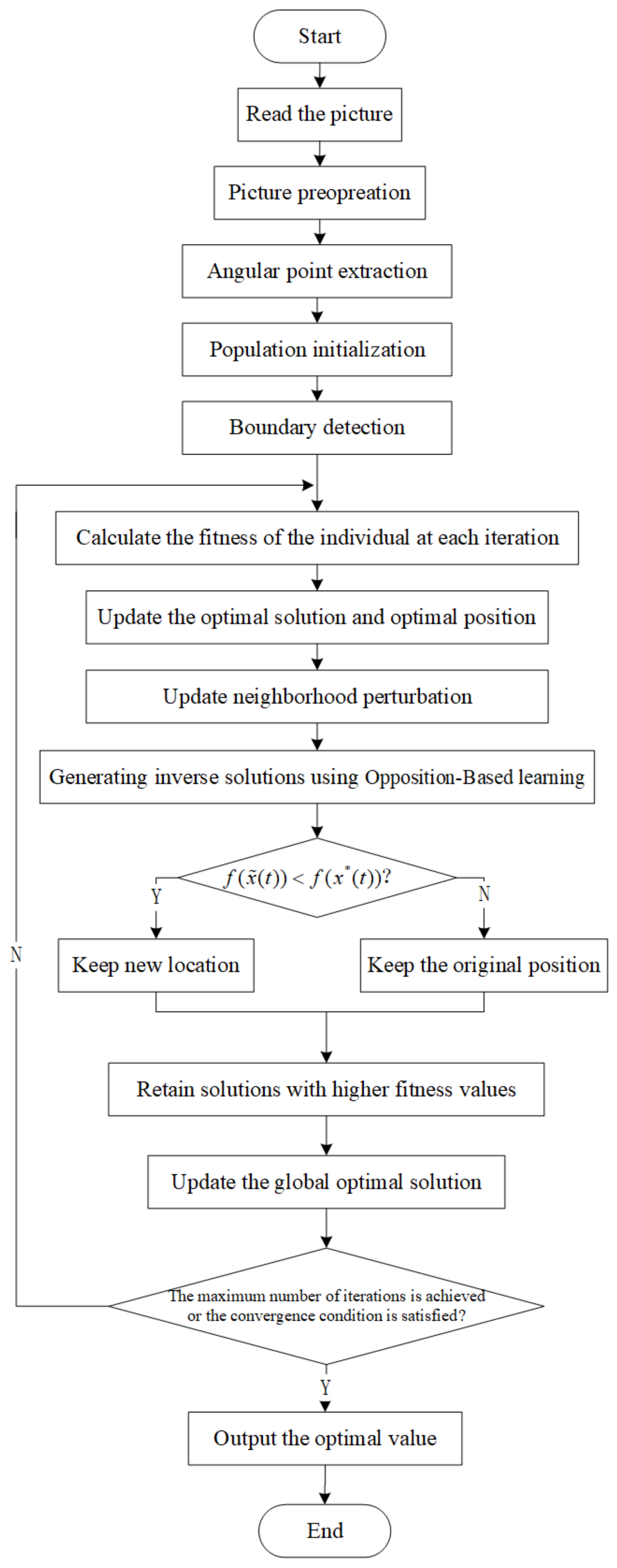
First, one must solve the initial values of the camera parameters $f_x$, $f_y$, $u_0$, $v_0$, $k_1$, $k_2$, $k_3$, $p_1$ and $p_2$, and then initialize the slime mold population to generate n different slime mold individuals. One must initialize the SMA algorithm and OBL algorithm, including the number of individuals in the population n, the size of search space and the number of iterations $Max\_t$. One must randomly select the initial positions of n slime molds, calculate the fitness value of each individual, implement the optimal neighborhood perturbation strategy for the current optimal individual to obtain a new current optimal individual, and then use the reverse learning strategy to solve the slime mold population, and select the solution with higher fitness to form a new slime mold population.

The fitness function is obtained from the objective function Equation (10), and the fitness function is defined by the following equation:

$$fitness=min{\displaystyle \sum _{i=1}^m\sqrt{{(x-u)}^2+{(y-v)}^2}}$$

(19)

where $(x,y)$ is the actual pixel coordinates obtained by the corner extraction algorithm; $(u,v)$ are the pixel coordinates obtained from the camera imaging relationship; m is the total number of corners.

The algorithm flow of camera internal parameter optimization using fusion algorithm is shown in Figure 1.

6. Experimental Verification

6.1. Experimental Scheme Design

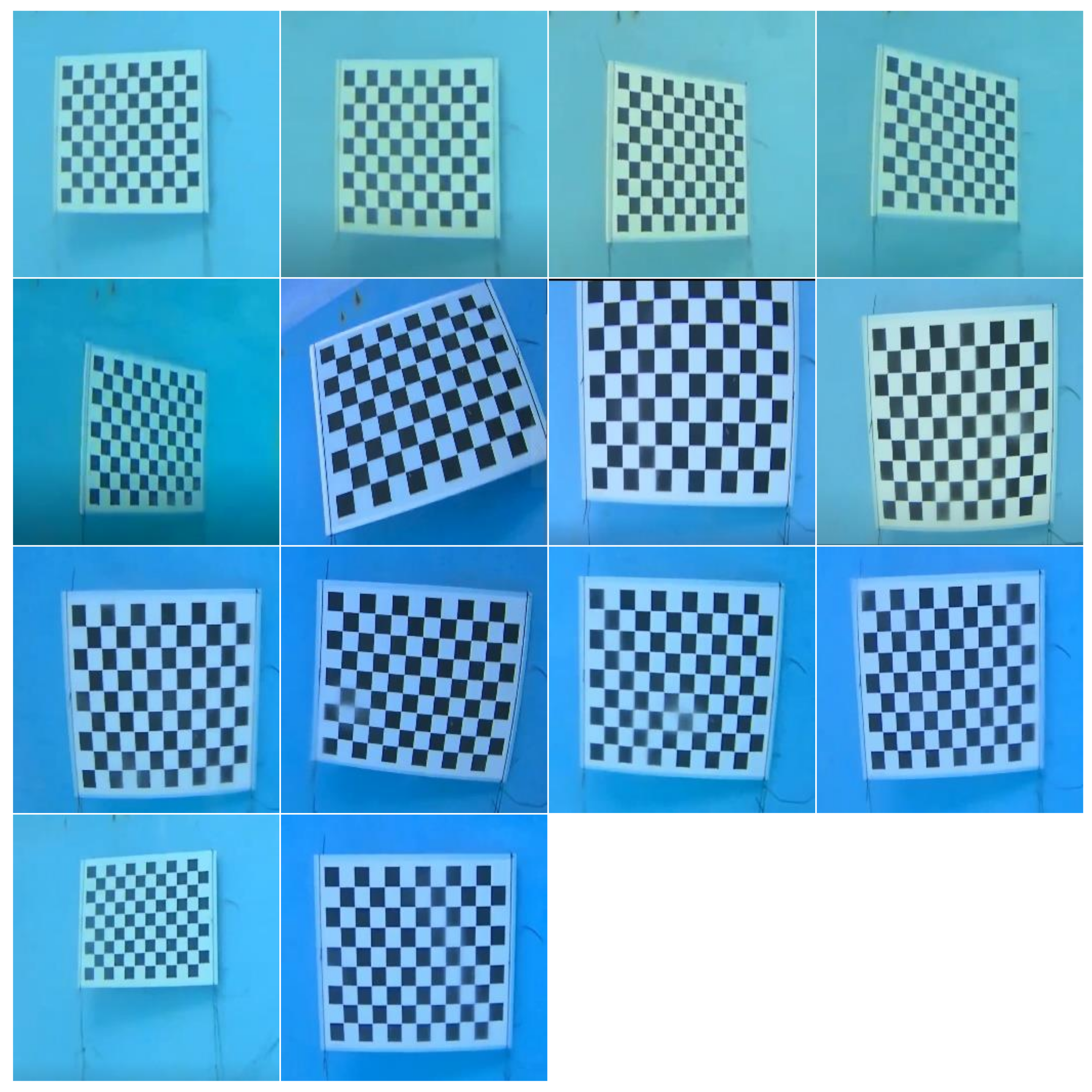
Using the hardware platform from the experiment, the camera has 200 W pixels, 110 field of view and 1080 p HD video real-time transmission. Python is used as the software development platform. The experimental environment of this paper is a 10 m × 10 m × 2 m pool, and the water in the pool is clear. The calibration board is immersed into the water and fixed on the pool wall, and the underwater camera is used to take pictures of the calibration board at different angles. A total of 20 pictures were taken, and the bad pictures caused by blurred pictures and incomplete display of the calibration board were deleted. The remaining 14 pictures were taken, and the internal parameters and distortion coefficient of the camera were calibrated based on these pictures. The pictures are shown in Figure 2 below.

The specific calibration steps were as follows:

Step 1: Realize the initial calibration of the camera based on Python OpenCV.

Step 2: Initialize the parameters according to Zhang’s calibration method.

Step 3: Bring in the slime mold algorithm to calculate the iteration results of 500 and 1000 times, respectively.

Step 4: Bring in particle swarm optimization algorithm and seagull algorithm to calculate the iteration results of 500 and 1000 times, respectively.

Step 5: Bring the initial parameters into the fusion algorithm and calculate the iteration results of 500 and 1000 times, respectively.

Step 6: Compare the results of the four algorithms.

6.2. Analysis of Experimental Results

Particle swarm optimization (PSO) [17] is a classical swarm optimization algorithm that was proposed earlier. The PSO algorithm can quickly approach the optimal solution and effectively control the parameters of the system. It also has the advantages of few parameters, simple algorithm and easy implementation. Seagull algorithm (SOA) [18] is an intelligent optimization algorithm that has been proposed in recent years. The population aggregation degree of SOA algorithm is low and the individual distribution is very scattered, which avoids the collision between individuals, expands the diversity of the population and improves the global search ability.

In this paper, fitness is chosen as the index to measure the merits of this method. Fitness refers to the relative ability of organisms in a population (compared to other genotypes) to survive and pass on their genes to the next generation. The more adaptable an organism is, the better the chance of survival and reproduction. In this paper, it is the reprojection error of camera calibration. In order to verify the performance of the fusion algorithm, SMA algorithm, SOA algorithm and PSO algorithm are selected in this paper, and their fitness curves are compared with those of the slime mold optimization algorithm (ORSMA), which combines optimal neighborhood interference and reverse learning strategies.

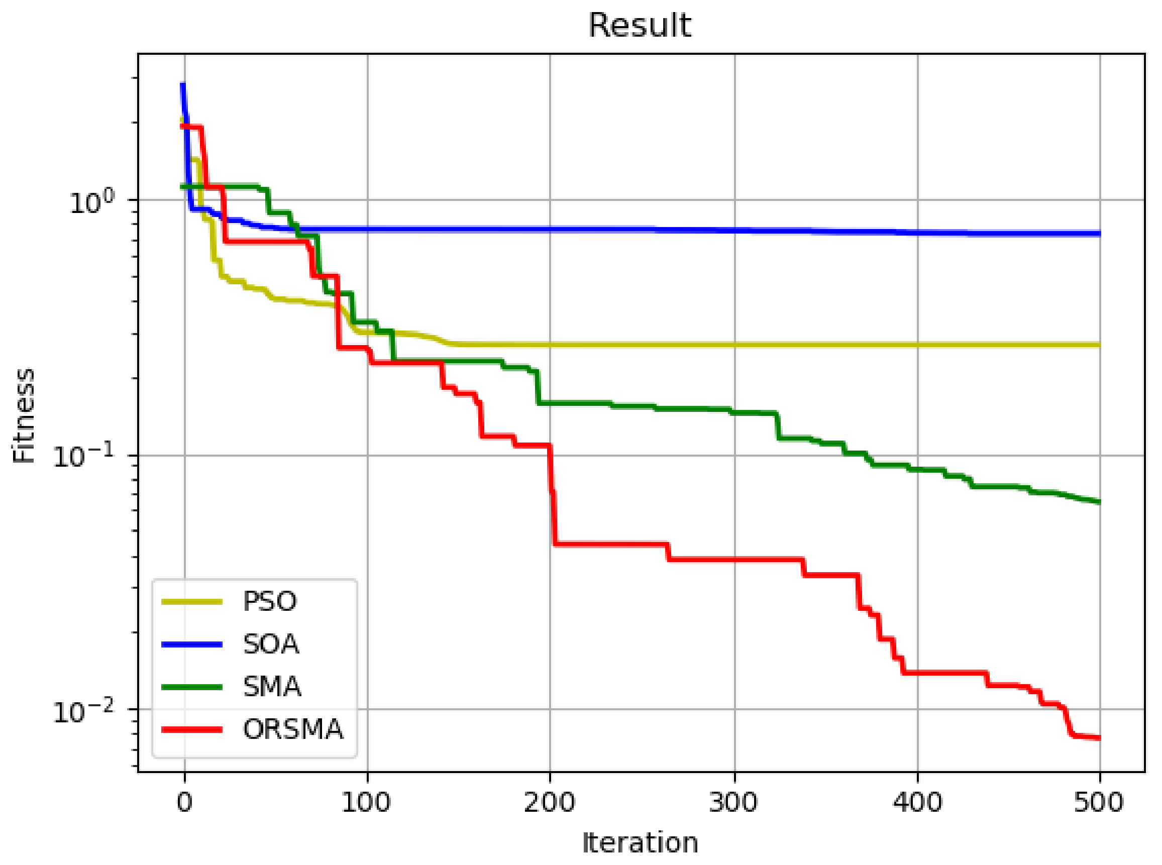
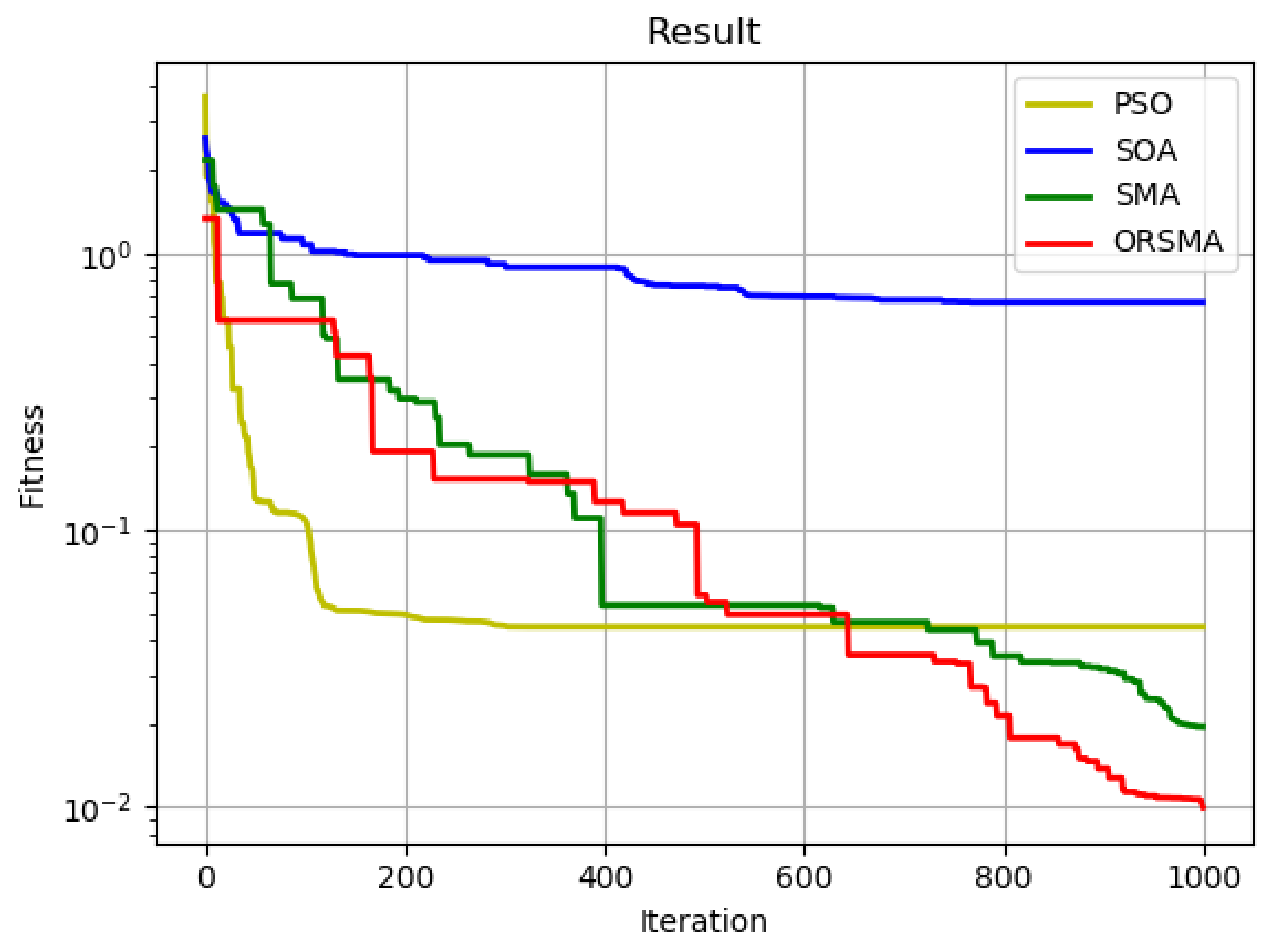
In this paper, the SMA algorithm, SOA algorithm, PSO algorithm and ORSMA algorithm are iterated 500 times and 1000 times, respectively. Within the iteration range of the two data, the difference of the fitness curves of the four algorithms can be observed very clearly, and the time cost is not too high. Figure 2 and Figure 3 show the results of 500 and 1000 iterations of the SMA algorithm, SOA algorithm, PSO algorithm and ORSMA algorithm, respectively. Among them, the yellow line represents the PSO algorithm, the blue line represents the SOA algorithm, the green line represents the SMA algorithm, and the red line represents the ORSMA algorithm. It can be observed from the figure that the SOA algorithm has the slowest convergence speed in the early stage, and it is very easy to fall into local optimization; the PSO algorithm has the fastest convergence speed and is easy to fall into local optimization. The early convergence curves of the SMA algorithm and ORSMA algorithm cross frequently, and they do not fall into local optimization. However, with the increase in the number of iterations, the convergence speed and accuracy of the ORSMA algorithm are significantly higher than that of the SMA algorithm and for ORSMA, it is more difficult to fall into local optimization.

Table 1. Calibration results of Zhang’s calibration method.

Parameter	Zhang’s Calibration Method
fx/pixel	1101.15390
fy/pixel	1189.31317
u0/pixel	203.673768
v0/pixel	150.846034
k1	−0.37039479
k2	0.18635836
p1	0.01825048
p2	0.0195527
k3	−0.09057577
Error	0.10989962

shows the internal parameters and distortion coefficients of camera calibration solved by Zhang’s calibration method.

Table 2. Camera internal parameter calibration results after 500 iterations.

Parameter	Method
	SOA	PSO	SMA	ORSMA
fx/pixel	601.15389965	1410.49484	1011.55162	1111.68207
fy/pixel	689.31316673	1336.40858	1089.72285	1192.76600
u0/pixel	216.65106585	197.063188	199.707583	203.615621
v0/pixel	77.64928307	171.234092	151.729567	119.276600
k1	13.62139211	−5.53713199	−3.04239425	−0.441324230
k2	14.87117853	−16.0303629	−9.05574467	1.14250554
p1	6.95762756	−0.530131156	0.258234732	0.00629919616
p2	−2.82293147	0.495974082	0.566243092	0.00004899095
k3	19.52709632	31.8425636	0.000000001	−0.519185085

and

Table 3. Camera internal parameter calibration results after 1000 iterations.

Parameter	Method
	SOA	PSO	SMA	ORSMA
fx/pixel	602.91076933	1042.34080	1114.04622	1103.90160
fy/pixel	691.32768149	1088.27820	1192.48902	1200.21466
u0/pixel	150.65135149	201.978786	202.772505	203.264646
v0/pixel	120.56691468	150.141963	150.265811	150.805549
k1	−33.57534433	−0.874402079	−4.16035531	−1.05483183
k2	−33.2041582	1.38275568	25.6283403	2.27889246
p1	6.92129933	0.361960909	0.134808315	0.0139799889
p2	3.61354862	0.141383928	0.118562365	0.0669686941
k3	7.32151031	−21.4787482	−49.7514346	−1.58430646

show the internal parameters and distortion coefficients of camera calibration solved by the SOA algorithm, PSO algorithm, SMA algorithm and ORSMA optimization algorithm for 500 and 1000 iterations, respectively, where $f_x$, $f_y$, $u_0$ and $v_0$ are the internal parameters and $k_1$, $k_2$, $k_3$, $p_1$ and $p_2$ are the distortion coefficients.

Table 4. Reprojection error.

Number of Iterations	Method
	SOA	PSO	SMA	ORSMA
500	0.48638793	0.05919811	0.01477718	0.00891584
1000	0.6670664	0.04475725	0.01948457	0.00998466

shows the reprojection error of the four algorithms after 500 and 1000 iterations, respectively. It can be observed from the table that the SOA algorithm greatly increases the reprojection error. The PSO algorithm, SMA algorithm and ORSMA algorithm have the optimization effect on the calibration results of Zhang’s calibration method, which can reduce the reprojection error. Among them, the ORSMA algorithm has the best optimization effect on the calibration results of Zhang’s calibration method. Figure 3 shows that in 500 iterations, the PSO algorithm, SMA algorithm and ORSMA algorithm reduce the reprojection error by 46.13%, 86.55% and 91.89%, respectively. Figure 4 shows that in 1000 iterations, the PSO algorithm, SMA algorithm and ORSMA algorithm reduce the reprojection error by 59.27%, 82.27% and 91.47%, respectively. When iterating 500 times and 1000 times, the ORSMA algorithm improves 35.76%, 5.34%, 32.2% and 9.2%, respectively, in the PSO algorithm and SMA algorithm. It can be observed that the performance of the ORSMA algorithm is better than SOA algorithm, PSO algorithm and SMA algorithm, and better calibration results can be obtained within the specified time.

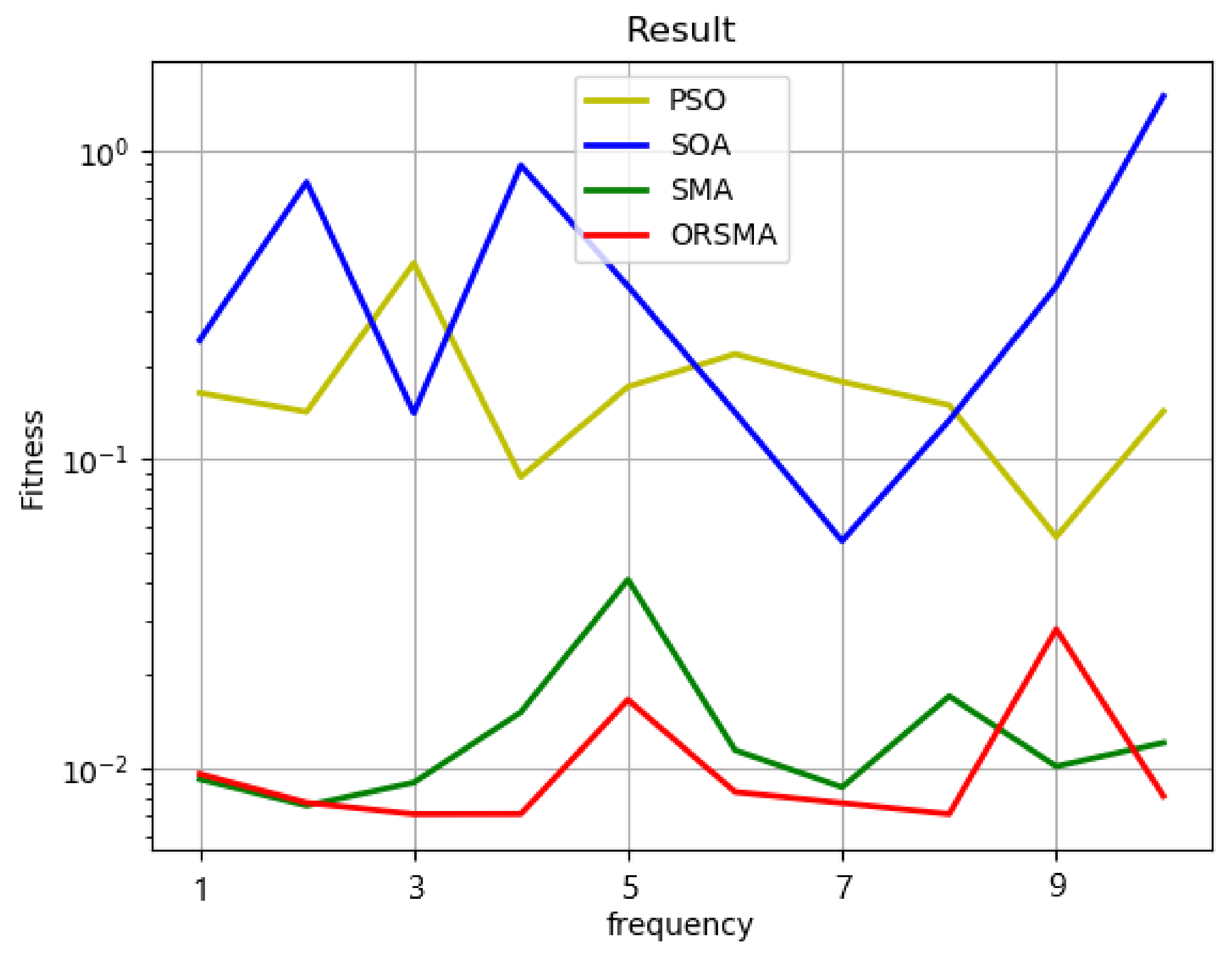
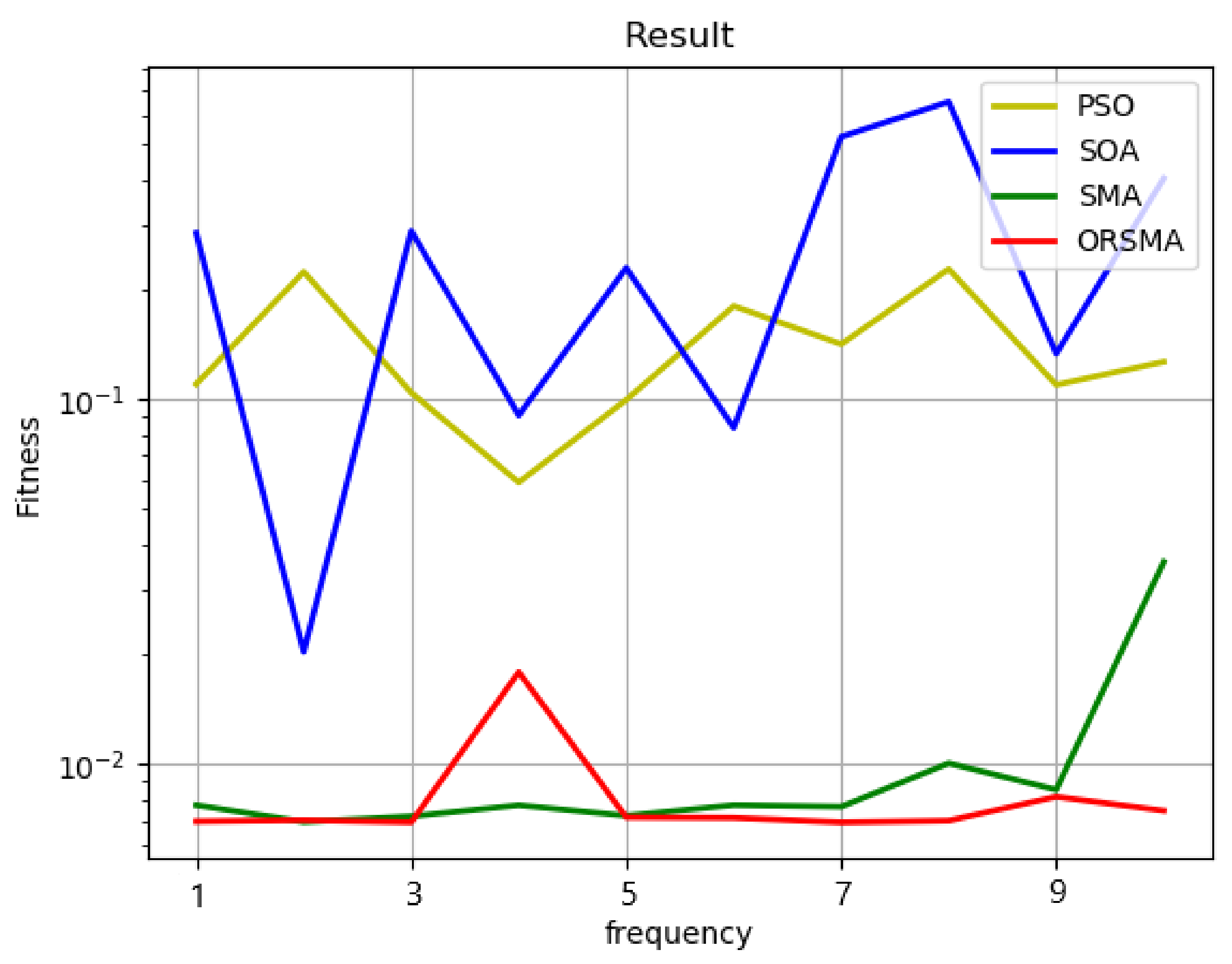
Evidently, the results obtained by processing PSO, SOA, SMA and ORSMA at one time are accidental, they do not have robustness and, when compared with other algorithms, the superiority of this algorithm on the camera calibration problem is not well proved. Therefore, in the calibration problem, the reprojection errors of the four algorithms after 500 and 1000 iterations are compared respectively. This process is repeated ten times. It can be observed from Figure 5 and Figure 6 that SMA and ORSMA are generally superior to PSO and SOA, and the effect of ORSMA is better than SMA. In the 10 times of processing results, ORSMA has three times and one time worse results than other algorithms. On the whole, ORSMA has the smallest fluctuation, followed by SMA, while PSO and SOA have sharp fluctuations in the 10 times of processing results. It can be observed that, compared with PSO, SOA and SMA, the ORSMA fusion algorithm has better robustness and stability in camera calibration, and the calibration accuracy is higher under the same conditions.

7. Conclusions

In this paper, a new camera calibration optimization method is proposed, which integrates the slime mold optimization algorithm, optimal domain interference algorithm and reverse learning algorithm into a framework according to certain rules. Aimed at the search ability of the low slime mold algorithm and the search speed after the decline in the problem, using the characteristics of optimal cell interference can improve the convergence speed and find a better global value of the optimal location near the region to avoid the “premature” phenomenon. The application of the OBL algorithm can also enlarge the searching range of the population and improve the searching ability. The reverse learning strategy was used to obtain the reverse solution of the population, retain the better slime molds, form new slime molds, and increase the diversity of the slime molds.

Compared with PSO and SMA, ORSMA reduces the camera calibration reprojection error by 32.2% and 9.2%, respectively. Compared with other algorithms, ORMSA has better stability and can be used stably for camera calibration optimization. The experimental results show that the ORSMA fusion algorithm has good accuracy and feasibility in the optimization of underwater camera internal parameters. This article for camera calibration optimization provides a new way to achieve stability and compared to the previous optimization algorithm applied in the field of camera calibration, the algorithm in the calibration precision is higher at the same time, the camera calibration process optimization has better stability, and can realize the stable optimization of camera calibration, unlike other algorithms with obvious contingencies. The algorithm can be applied stably to solve nonlinear optimization problems in engineering examples. On the basis of higher calibration accuracy, it is more beneficial to improve the accuracy of 3D reconstruction, target recognition and other applications. In the next step, we will try to establish underwater imaging models or improve existing underwater imaging models, use intelligent optimization algorithms to solve the problems existing in these models, and verify the calibration accuracy and efficiency in underwater environments.