Article

A New Collaborative Multi-Agent Monte Carlo Simulation Model for Spatial Correlation of Air Pollution Global Risk Assessment

by
Mustafa Hamid Hassan
1,2,
Salama A. Mostafa
1,*,
Aida Mustapha
3,
Mohd Zainuri Saringat
1,
Bander Ali Saleh Al-rimy
4,
Faisal Saeed
5,
A.E.M. Eljialy
6 and
Mohammed Ahmed Jubair
1,2
1
Faculty of Computer Science and Information Technology, Universiti Tun Hussin Onn Malaysia, Parit Raja 84600, Malaysia
2
College of Information Technology, Imam Ja’afar Al-Sadiq University, Al-Muthanna 66002, Iraq
3
Faculty of Applied Sciences and Technology, Universiti Tun Hussein Onn Malaysia, Panchor 84500, Malaysia
4
School of Computing, Faculty of Engineering, Universiti Teknologi Malaysia, Johor Bahru 81310, Malaysia
5
School of Computing and Digital Technology, Birmingham City University, Birmingham B4 7XG, UK
6
Department of Information System, College of Computer Engineering & Sciences, Prince Sattam Bin Abdulaziz University, Alkharj 11942, Saudi Arabia
*
Author to whom correspondence should be addressed.
Sustainability 2022, 14(1), 510; https://doi.org/10.3390/su14010510
Submission received: 29 October 2021 / Revised: 25 December 2021 / Accepted: 27 December 2021 / Published: 4 January 2022

Abstract

:
Air pollution risk assessment is complex due to dynamic data change and pollution source distribution. Air quality index concentration level prediction is an effective method of protecting public health by providing the means for an early warning against harmful air pollution. However, air quality index-based prediction is challenging as it depends on several complicated factors resulting from dynamic nonlinear air quality time-series data, such as dynamic weather patterns and the verity and distribution of air pollution sources. Subsequently, some minimal models have incorporated a time series-based predicting air quality index at a global level (for a particular city or various cities). These models require interaction between the multiple air pollution sensing sources and additional parameters like wind direction and wind speed. The existing methods in predicting air quality index cannot handle short-term dependencies. These methods also mostly neglect the spatial correlations between the different parameters. Moreover, the assumption of selecting the most recent part of the air quality time series is not valid considering that pollution is cyclic behavior according to various events and conditions due to the high possibility of falling into the trap of local minimum and poor generalization. Therefore, this paper proposes a new air pollution global risk assessment (APGRA) prediction model for an air quality index of spatial correlations to address these issues. The APGRA model incorporates an autoregressive integrated moving average (ARIMA), a Monte Carlo simulation, a collaborative multi-agent system, and a prediction algorithm for reducing air quality index prediction error and processing time. The proposed APGRA model is evaluated based on Malaysia and China real-world air quality datasets. The proposed APGRA model improves the average root mean squared error by 41%, mean and absolute error by 47.10% compared with the conventional ARIMA and ANFIS models.

1. Introduction

Air quality has drawn much attention in recent years because it seriously affects people’s health. At present, monitoring stations in a city can provide real-time air quality measures [1]. Nonetheless, people strongly desire air quality prediction, which is challenging as it depends on several complicated factors, such as weather patterns and spatial-temporal dependencies of air quality. Air pollution risk assessment is complex due to its dynamic data and distributed pollution sources [2]. For instance, predicting air quality on weekdays and weekends may be different due to the difference in anthropic emissions [3]. Air Quality Index (AQI) effectively protects public health by communicating early warnings of harmful air pollutants. However, the prediction is challenging because it depends on several complex factors, such as weather patterns, nonlinear time series of air quality data, and distribution of air pollution sources [4,5]. The dynamic data and distributed air pollution risk assessment sources need to be estimated relying on two phases. The first phase is utilized to predict the AQI of a local area. The second phase is employed to assess the global risk level based on the AQIs of local areas [6,7].
Air quality prediction aims to predict the future state of air quality in a specified location based on existing data, like historical air quality and meteorological data. Many types of research have been conducted to tackle the problem of assessing air pollution risk. Some examples are the works of [4,7,8]. Each of these has mostly focused on assessing the concentration of a specific pollutant parameter such as PM2.5, CO, and PM10 [7,9]. However, some approaches have been focused on predicting the level of certain parameters that directly impact the state of pollution [6,10]. The literature provides a significant number of works in air pollution prediction models either for a specific location or specific variables. Feng et al. [11] combine air mass trajectory analysis and wavelet transformation with artificial neural network (ANN) to improve the prediction accuracy of daily average concentrations of PM2.5. Tong et al. [8] deploy Monte Carlo simulation (MCS) to estimate health risks related to the concentration of dust-induced occupational conditions.
Prasad et al. [12] used an adaptive neuro-fuzzy inference system (ANFIS) for predicting the concentration of several AQI parameters. However, these models predict air pollution concentrations based on the most recent part of the time series. This mechanism requires larger data for producing proper prediction results. It is highly possible to fall into the trap of local minimum [4,10]. Moreover, the learning or training of these models with short-term prediction situations may never converge due to the training data/time insufficiency, which might cause the algorithms to be trapped in an infinite training situation [13]. Because of these constraints, the statistical approach represents the best option. One of the best statistical approaches that deal with short-term time series prediction is the autoregressive integrated moving average (ARIMA) algorithm, as it only requires prior data of a time series to generalize the prediction of the AQI model [4]. However, the ARIMA algorithm does not produce satisfactory results for certain air pollution parameters (i.e., PM10 and CO), even for a short prediction period [14,15,16].
Many approaches have tackled the problem of weather variable prediction and forecasting as well as pollution estimation and alarming. Each one has concentrated on one aspect, while some strategies have focused on predicting the level of a certain variable that has a critical impact on the pollution state [6]. Others have dealt with the issue of lacking adequate measurement stations across countries [9]. Moreover, some approaches have focused on building models for estimating air pollution more accurately based on feature selection or neural networks. Others have built one-step-ahead forecasting models [11,14,15] and have used fuzzy models for alarming air pollution [4,7]. Hence, a set of neural networks and simple auto-regression forecasters can be used, such as in the work of Westerlund et al. [17] that is validated to be superior over a single forecaster. The literature has revealed that very limited models have been constructed to assess the global (interaction between the pollution sources) level of air pollution. However, the dynamic nature and high spatiotemporal variability of AQI represent a complex predicting problem. Hence, none-of the existing models are able to incorporate time-series data to provide dynamic forecasting of various weather variables. This can be achieved by tackling the global interaction of different locations using wind direction and speed for enabling contextual forecasting added to the mathematical model. Consequently, the research gap lies in the absence of interaction between air pollution parameters under investigation and finding the global prediction level of the dynamic and distributed air pollution risk.
This paper identifies that the global interaction among meteorological parameters such as wind speed and wind direction at the different areas is essential in air pollution prediction and risk assessment due to the nature of dynamic weather and air pollution time series at various locations. The study in this paper aims to fill this gap by searching for ways to overcome the conditional heteroscedasticity problem. The contributions of this paper are represented by: (i) to develop ARIMA-based MCS prediction algorithm that integrates ARIMA and MCS algorithms for reducing AQI prediction error; (ii) to propose an air pollution global risk assessment (APGRA) model that incorporates the ARIMA-based MCS algorithm into a multi-agent system (MAS) for dynamic and distributed assessment of multiple sources of AQI risk levels; and (iii) to test and evaluate the performance of APGRA models in terms of prediction error and time by using China and Malaysia air quality datasets.
The remaining parts of the paper are organized as follows: Section 2 provides Materials and Methods. Section 3 describes the Monte Carlo method to be used in accommodating the uncertainty of the forecast. It then presents a proposed APGRA model. Section 4 discusses the results of the APGRA model, and Section 5 provides conclusions and future research.

2. Materials and Methods

This section covers the materials and methods which are used in this paper. At the same time, it first explains the air pollution datasets divided into two case studies: Malaysia and China. Second, it explains the prediction algorithms that are used in the local risk assessment, such as MCS and ARIMA. Third, it explains several performance measures such as root mean square error (RMSE) and mean absolute error (MAE) used to evaluate this work.

2.1. Air Pollution Datasets

This study utilizes two real-world air pollution datasets of Malaysia and China. The data layout is presented as a matrix D = { x t i , j } , where i = 1 , 2 M , j = 1 , 2 N , M indicates the number of variables, and M indicates the number of cities, t represents the time, sampled as hourly. The data is fed into the framework for one of two goals, forecasting one of the time series within a certain defined time horizon or evaluating a given model configuration in terms of its forecasting accuracy in a certain time interval. Another element of the data is the map combined with longitude and latitude for all cities with their time series included in matrix D. The datasets are described in the following subsections.

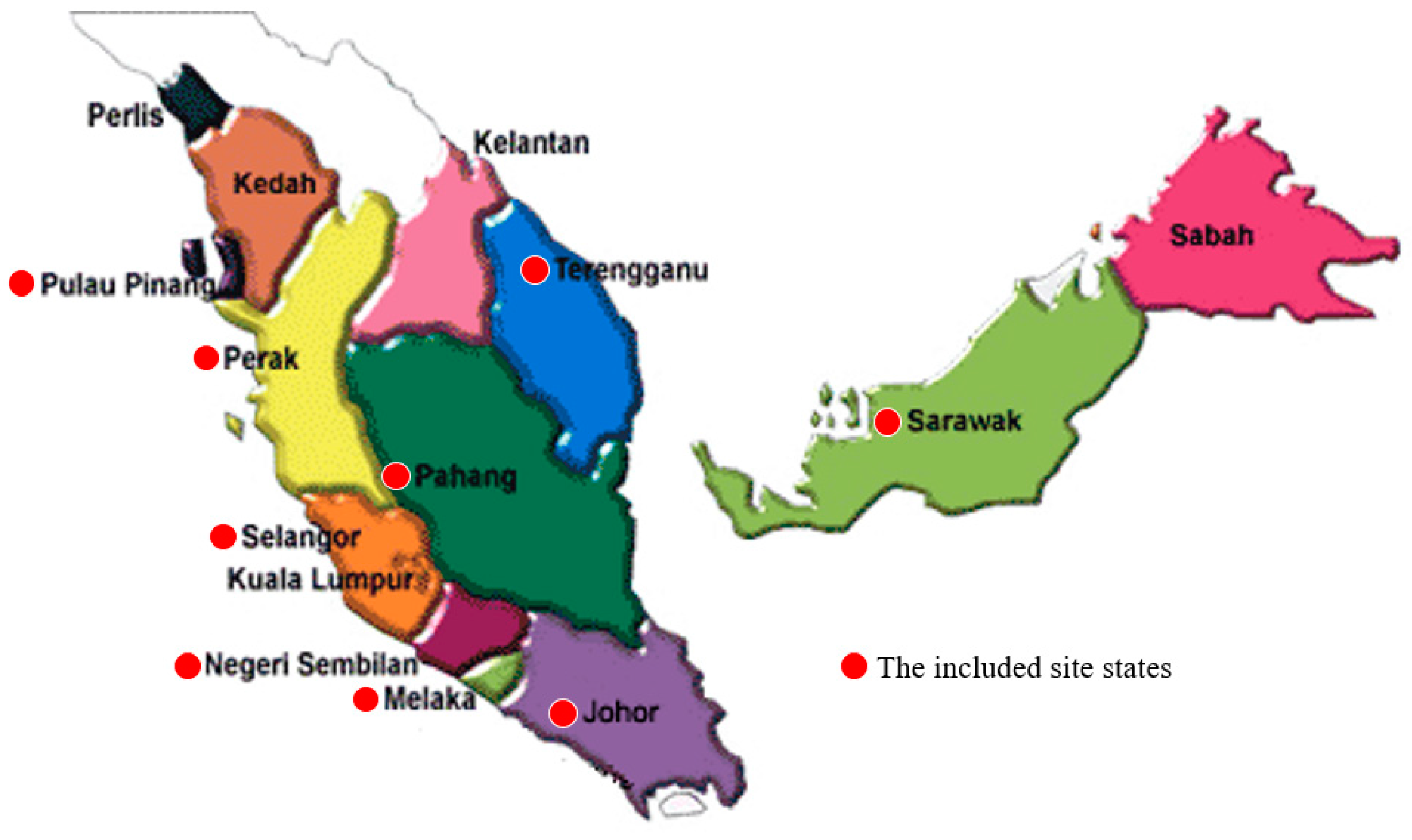
2.1.1. Malaysia Air Pollution Dataset

This paper applies the heterogeneous data set, including the one-dimension series data and the multi-dimension panel data. The one-dimension series data is composed of the value of AQI concentrations with the change of time. For the panel data, the Sulphur Dioxide (SO2), Nitrogen Dioxide (NO2), Carbon Monoxide (CO), Sulfur Dioxide (SO2,) and Ozone (O3) concentrations, temperature, relative humidity (RH), wind speed (WS), and PM10 concentrations of the previous hour are selected as the input variables. The AQI concentrations of the current hour are the output variable of the forecasting model. The Malaysia air quality monitoring network gathers the PM10, SO2, NO2, CO, and O3 concentrations data. The air quality monitoring stations include ten stations, as illustrated in Figure 1.
The data of air pollutant concentrations are collected from the different cities of Malaysia. Table 1 shows the locations of the included states in this study. Hourly air quality data have been collected from the eight air pollution monitoring stations during the ten years from 2006 to 2016 in Malaysia. These stations record data of some important AQI parameters such as the CO, NO2, O3, and “Particulate Matter (PM10)”. These parameters are used to calculate the AQI. AQI is a commonly used indicator defined by the United States Environmental Protection Agency (EPA) to use air quality conditions. In order to calculate AQI for a location, an indicator value of AQI is calculated for each of the observed pollutant concentrations (CO, NO2, O3, and PM10) using Equation (1) [18].
A Q I = I h i g h I l o w C h i g h C l o w   ( C     C l o w   ) + I l o w  

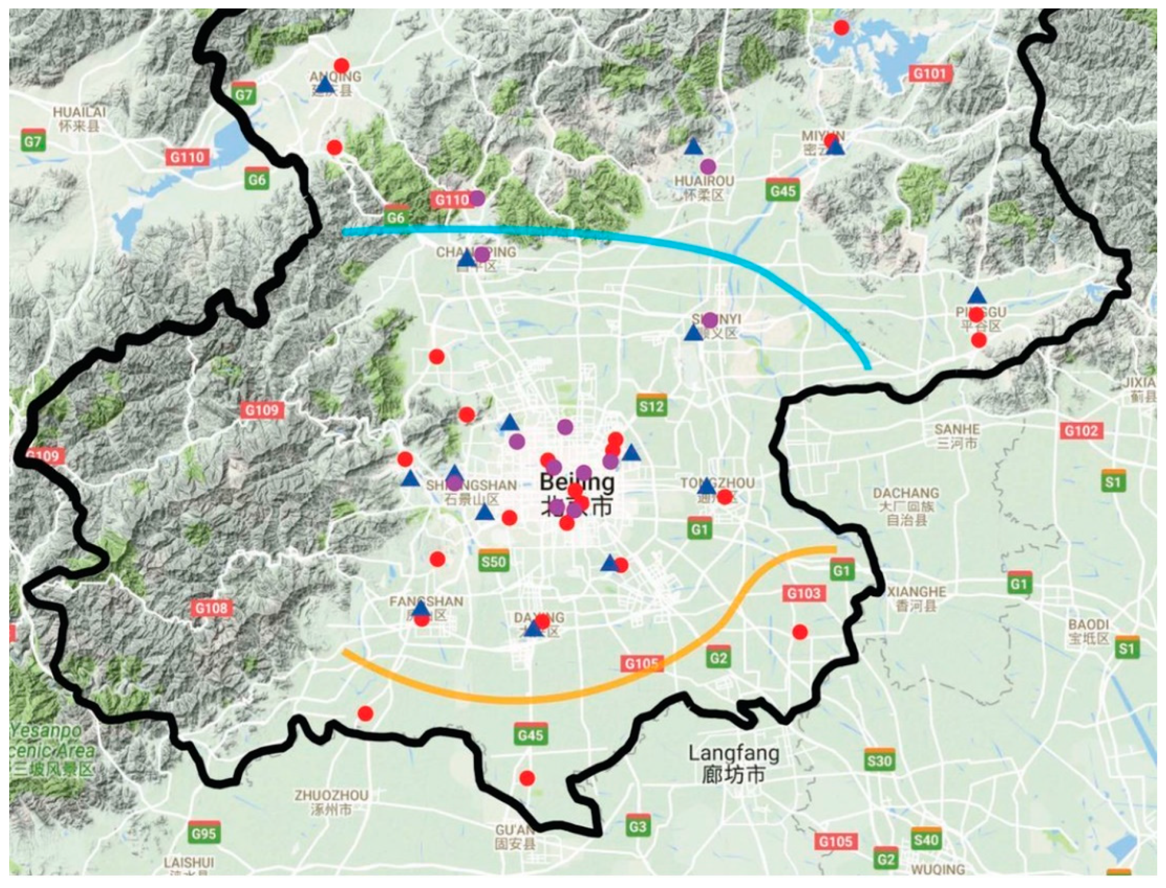
2.1.2. China Air Pollution Dataset

The Beijing multi-site air-quality dataset comprises hourly AQI parameters from 10 measured air pollution monitoring locations countrywide [1]. The AQI data characterizes the Beijing public environmental areas for the 24-h care center. The climatological and meteorological data in the AQI site are coordinated with China’s climatological management’s adjacent climate monitoring site. The historical time is from March 2013 to February 2017. Table 2 and Figure 2 show descriptive information related to the dataset.
The response AQI is classified into four categories: AQI ≤ 35 μgm−3 (green), 35 μgm−3 < PM2.5 ≤ 75 μgm−3 (yellow), 75 μgm−3 < AQI ≤ 150 μgm−3 (orange) and AQI > 150 μgm−3 (red). The four numbers inside each colored node indicate the proportions of the AQI categories at each layer of the branch, and the percentage represents the marginal proportion of the sample at the node. Figure 2 shows the position of 36 air quality monitoring sites marked as purple and red circles and 15 metrological sites marked as blue triangles.

2.2. Prediction Methods

2.2.1. Descriptive Statistics

Descriptive statistics are used to quantitatively describe or summarize each monitoring station data’s features for further explaining their implication. Mean and median are statistical terms introduced to understand the central tendency of the data. Minimum and maximum show the amplitude of the time series. Standard deviation is a measure for quantifying the amount of variation or dispersion of the data values. A low standard deviation indicates that the data points tend to be close to the data set’s mean, while a high standard deviation indicates that the data points are spread out over a wider range of values. Skewness and kurtosis are applied to judge whether the sampling distribution is normal or not. Moreover, standard error of skewness (SES) and standard error of kurtosis (SEK) are presented to show the deviation between Skewness or Kurtosis’s values.

2.2.2. ARIMA Algorithm

ARIMA, short for the auto-regressive integrated moving average, is actually a class of models that explains a given time series based on its own past values, that are its own lags and the lagged forecast errors so that the equation can be used to forecast future values. Any ”non-seasonal” time series that exhibits patterns and is not a random white noise can be modeled with ARIMA models [4]. An ARIMA model is characterized by three terms: p, d, and q. Where p is the order of the AR term, q is the order of the MA term, and d is the number of differences required to make the time series stationary. If a time series has seasonal patterns, then seasonal terms are added, becoming SARIMA, short for seasonal ARIMA. The first step to building an ARIMA model is to make the time series stationary because the term “Auto Regressive” (AR) in ARIMA means it is a linear regression model that uses its own lags as predictors. Linear regression models work best when the predictors are not correlated and are independent of each other. The most common approach is to subtract the previous value from the current value. Sometimes, depending on the complexity of the series, differences might be needed. Therefore, the value of d is the minimum number of differences needed to make the series stationary. If the time series is already stationary, then d = 0. “p” is the order of the AR term. It refers to the number of lags of Y to be used as predictors. And “q” is the order of the “Moving Average” (MA) term. It refers to the number of lagged forecast errors that should go into the ARIMA Model. We adopt for forecasting the famous ARIMA model that is given by the Equation:
d I x t i , j = α 1 d I x t 1 i , j + α 2 d I x t 2 i , j + α p d I x t p i , j + u t + β 1 u t 1 + β q u t q  

2.2.3. Monte Carlo Simulation

Monte Carlo simulation (MCS) algorithms are mainly used in three problem classes: optimization, numerical integration, and generating draws from a probability distribution. MCS is one of the most common methods used to accommodate the uncertainties associated with many risk-related problems [8,19,20]. It has been recognized as a means of quantifying variability and uncertainty in risk assessments by the National Academy of Sciences and USEPA. This method provides a quantitative way to estimate the probability distributions for exposure risks and provides more information for making decisions related to risk protection. The widespread use of MCS in risk assessment promises a significant improvement in the scientific rigor of these assessments [20]. The MCS method generally requires three main steps, which are intended as follows:
Step 1 Construct a descriptive procedure to the probabilistic process:
  • Build an appropriate probability model according to the simulated object’s characteristics;
  • Find a suitable distribution function to the desired solution.
Step 2 Achieve sampling method from a known probability distribution:
  • Generate a random variable (or random vector) with a known probability distribution;
  • Generate a random variable of a sample;
  • Establish the sampling method of the random distribution.
Step 3 Establish various statistical estimators:
  • Simulate a random variable as the solution to the object problem;
  • Find the unbiased estimator.
Many statistics problems involve nested expectations and thus do not permit conventional MCS estimation. For such problems, a nest estimator, terms in an outer estimator, involve calculating a separate and nested expectation [19]. Nested expectations occur in a wide variety of portfolio risk management problems [21]. Tackling such problems requires some form of nested estimation scheme in the MCS. In this approach, MCS simulated as an interest in estimating quantities of the form:
E Z = [ F ( E ( W | Z ) ]  
where Z represents deferent risk scenarios, and E[W|Z] represents exposure, depending on the scenario.

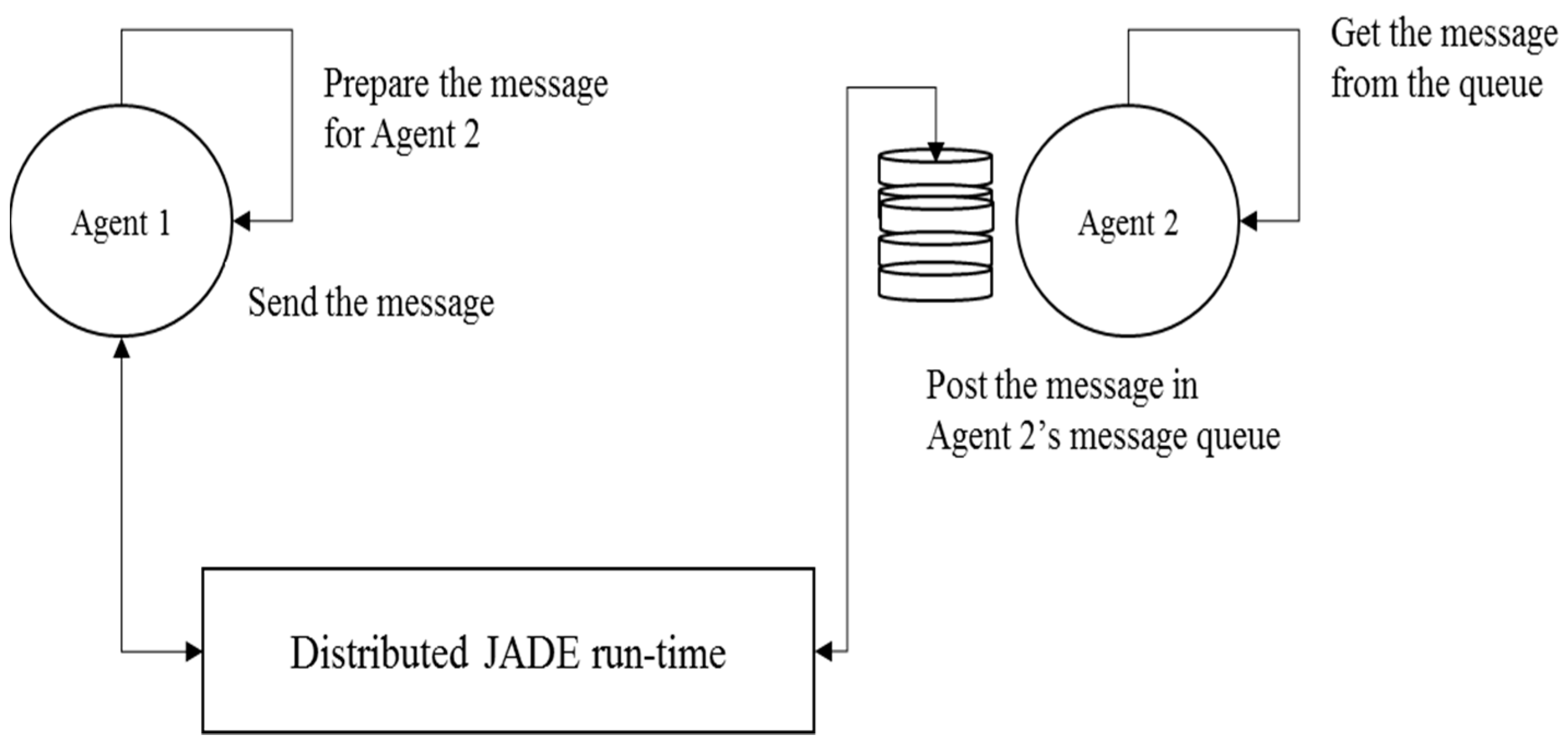
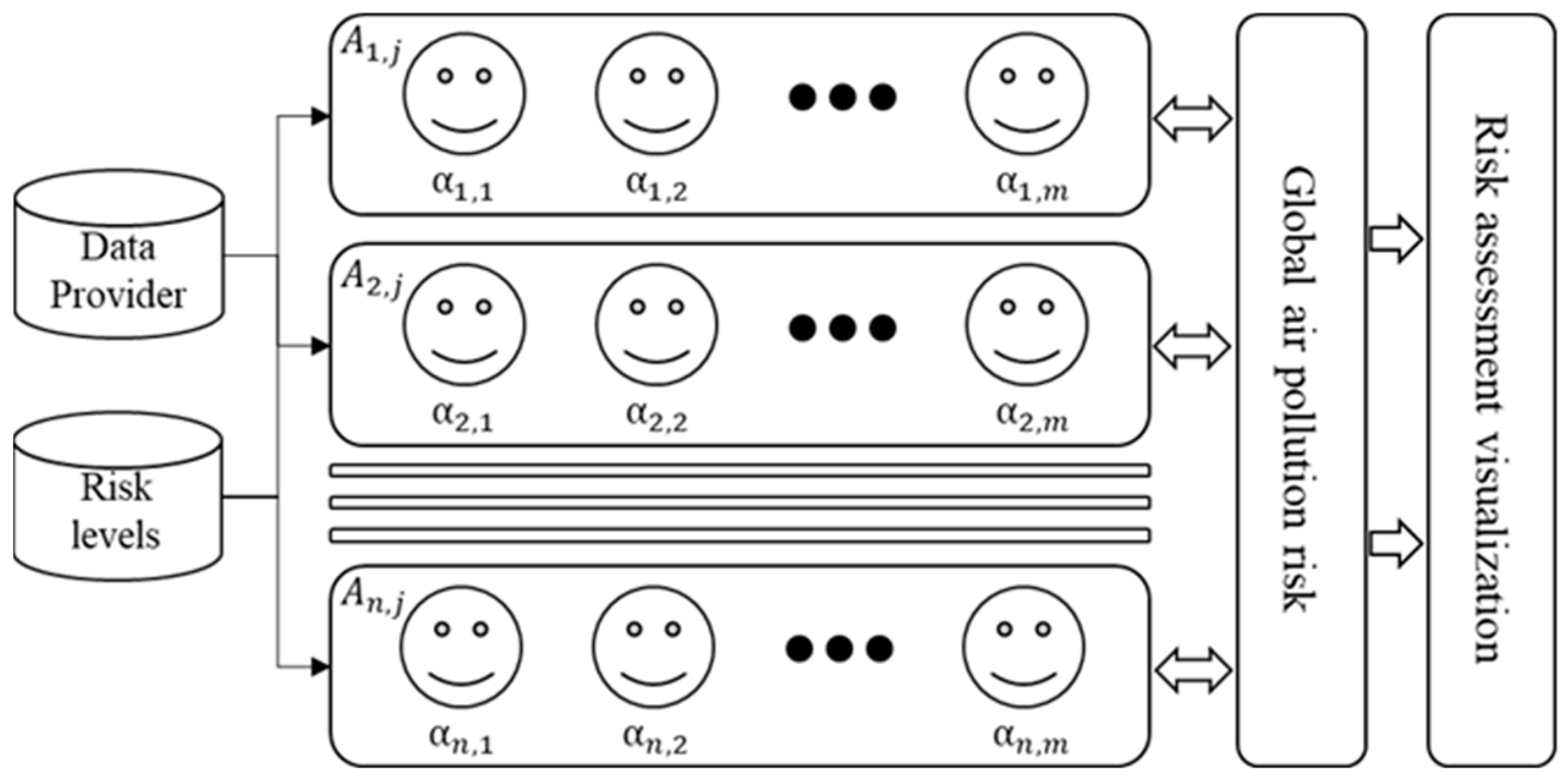
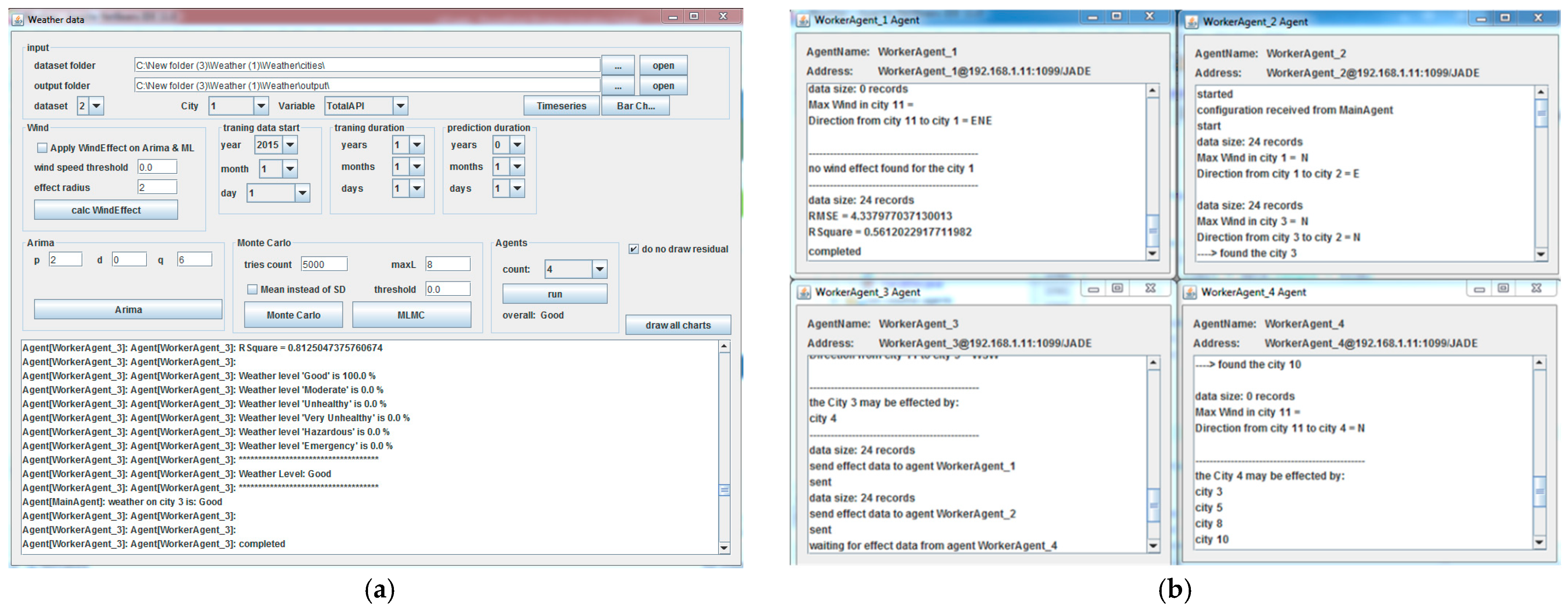
2.3. Modeling Dynamic and Distributed Behavior

Dynamic and distributed problem solving is achieved by employing a MAS that has the behaviors and methods of interaction, communication, and collaboration [22,23]. The dynamic behaviors of the agent help the statistical methods such as ARIMA or MCS to perform dynamic prediction tasks and assess the risk with the availability of dynamic data sources [24,25]. The term “agent”, or software agent, has found its way into many technologies and has been widely used, for example, in artificial intelligence [26], data processing [25], operating systems [27], and healthcare and computer networks [28] literature. An agent can execute several behaviors concurrently. However, it is important to note that the scheduling of behaviors in an agent is collaborative rather than preemptive (as for running threads). This means when behavior is scheduled for execution, its action method is not called but runs until it returns, dynamically deliberating the selection of action options based on the agent and the environmental conditions [22,29].
The problem of distributed risk assessment, however, depends on the communication agent and collaboration features. Each agent represents a location or city in multiple city environments in which the agents need to communicate with each other to assess the global risk of air pollution [23,30]. Agent communication is probably the most utilized feature of the Java Agent Development Framework (JADE) [31]. The communication paradigm is based on asynchronous message passing. Thus, each agent has a “mailbox” (the agent message queue) where the JADE run-time posts messages sent by other agents [30]. The receiving agent is notified whenever a message is posted in the mailbox message queue. However, the agent picking up the message from the queue for processing is a design choice of the agent programmer. This process is depicted in Figure 3.
Each message includes the following fields: (i) the sender of the message; (ii) the list of receivers; and (iii) the communicative act (also called the “performative”) indicating what the sender intends to achieve by sending the message. For instance, if the performative is REQUEST, the sender wants the receiver to act, if it is INFORM, the sender wants the receiver to be aware of a fact. The content containing the actual information to be exchanged by the message (e.g., the action to be performed in a REQUEST message, or the fact that the sender wants to disclose in an INFORM message, etc.). The content language indicates the syntax used to express the content. Both the sender and the receiver must be able to encode and parse expressions compliant with this syntax for the communication to be effective.

2.4. Evaluation Metrics

In order to evaluate the performance of a forecasting system, we use several model performance measures such as MAE, RMSE [25]. The formulas of the statistical measures used herein are as follows:
M A E = 1 n i = 1 n | Y i y i |
R M S E = i = 1 n ( Y i y i ) n
Y i and y i are the forecast value and the observed value, respectively. MAE and RMSE are applied as the performance criterion of the prediction model to quantify the errors of forecasting values. In general, the smaller the values, the better the prediction or the closer the estimator approaches the actually observed ones.

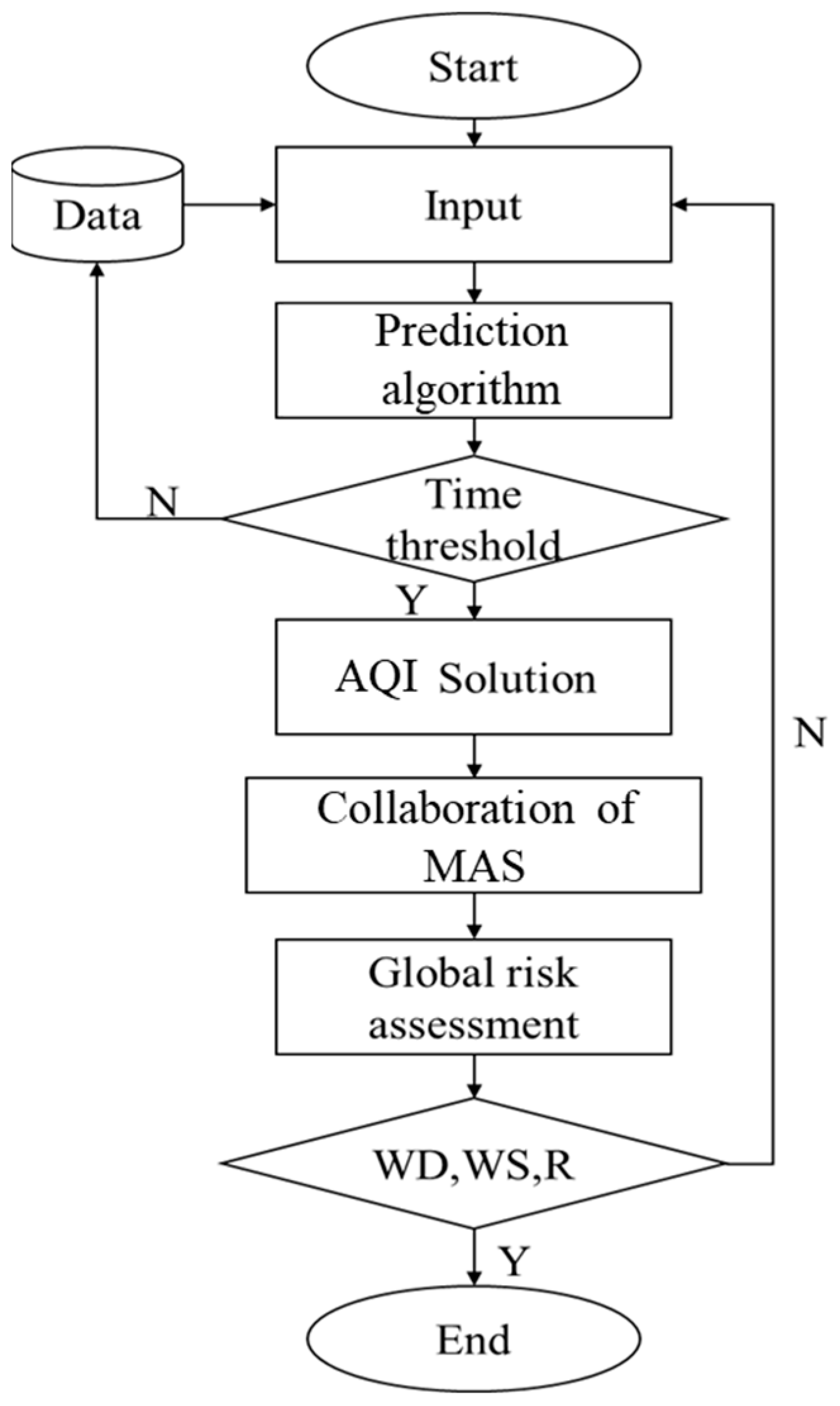
3. Air Pollution Global Risk Assessment (APGRA) Model

The Air Pollution Global Risk Assessment (APGRA) model consists of local air pollution risk assessment and Global air pollution risk assessment. The local air pollution risk assessment has an improved ARIMA-based MCS algorithm that performs local forecasting to the AQI risk of a particular area or city. Subsequently, in the Global AQI risk assessment, the APGRA model offers more accurate and global-oriented AQI forecasting through deploying MAS architecture in which agents are controlling the ARIMA-based MCS algorithm of cities. The APGRA model performs based on agent interaction and processing of the AQIs’ parameters.

3.1. Air Pollution Local Risk Assessment

This section explains the usage of the MCS to accommodate the uncertainty of the forecasting method presented in the ARIMA-based MCS algorithm. The concept of using MCS is to exploit the repeated sampling of the operation of the ARIMA outcomes to provide a more accurate description of the forecasting results of the local air pollution risk assessment. The ARIMA-based MCS algorithm defines a set of parameters that describe our usage of the MCS. Firstly, the algorithm selects the time interval that is used to fit the simulation model. The ARIMA(p, I, q, i, j) function has the p, q, I, which are the same as presented earlier, and i, j represents the subject time series type and city that is under simulation. Secondly, the algorithm selects the time interval T_past that is used for fitting ARIMA(p, I, q, i, j), and users assign it. Thirdly, the ARIMA-based MCS algorithm selects the time horizon T_future that the forecasting model uses. Fourthly, the algorithm selects the number of runs N_runs that MCS uses.
Algorithm 1 shows the ARIMA-based MCS. The main task of the MCS is to execute the forecasting of the ARMIA that is fitted in the requested T _ p a s t for the requested T _ f u t u r e . This procedure is repeated several times equal to N_runs, representing the number of simulations. After accumulating all the forecasted time series, we calculated the random process summarized by the distribution of the predicted time series. Assuming that the distribution is normal, the ARIMA-based MCS algorithm offers two series, y_forecasted, which provides the forecasted time series, and σ_forecasted, which provides the indicator of the confidence or risk of the local AQI forecasting.
Algorithm 1 Air Pollution Local Risk Assessment Algorithm
Input
   initial input < ARIMA (p, I, q, i, j); T_past; T future; N_runs; y_history >;
   initial output < y_forecasted, σ_forecasted >;
Output
   Y = []; y_forecasted; σ_forecasted;
Start
   prediction model = fitARIMA (p, I, q, i, j, T_past, N_runs, y_history);
   for t = 1 until No_runs do:
   y_forecasted = forecast (model, T_past, T_future);
   Y = add(y_forecasted);
end
   σ_forecasted = sqrt(variance(Y));
   y_forecasted = avg(Y);
End

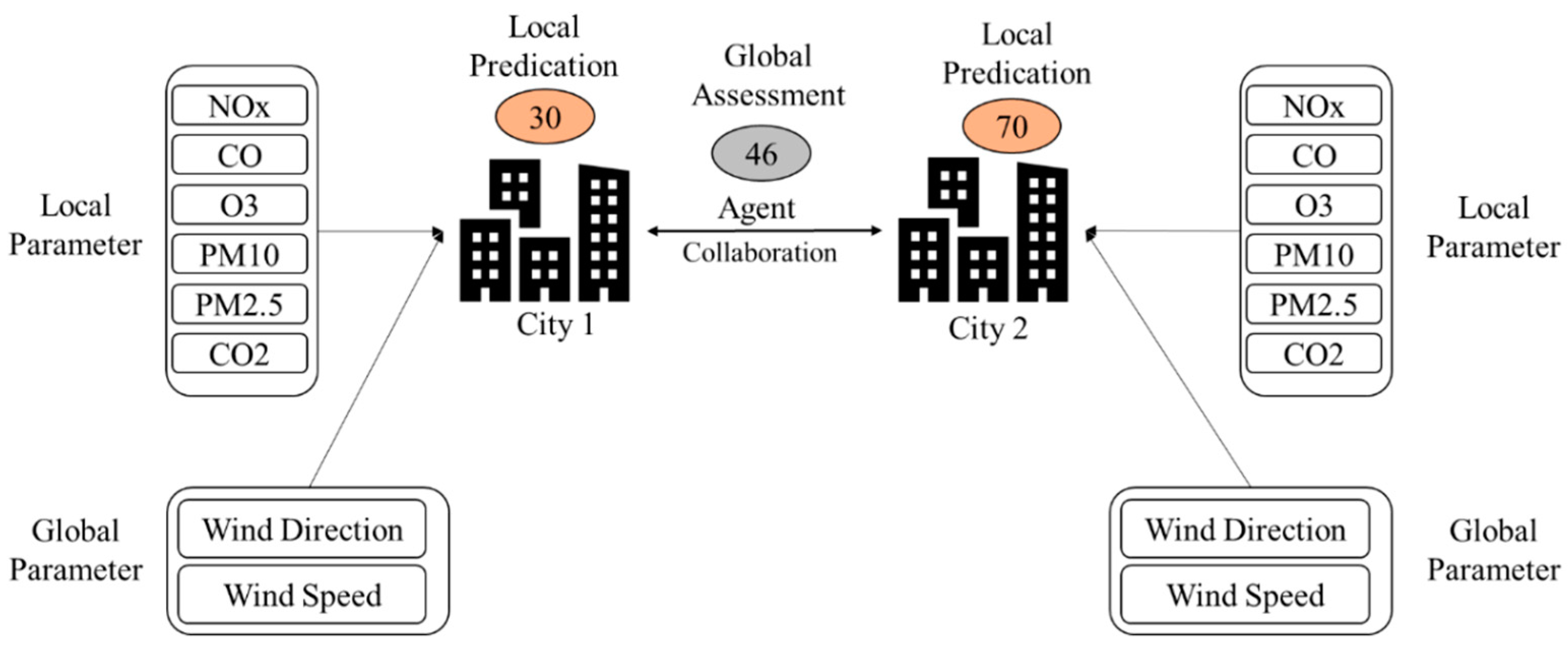
3.2. Air Pollution Global Risk Assessment

The issue with the previous algorithm of the ARIMA-based MCS algorithm is its non-awareness of the global aspect regarding possible interaction between individual cities. In order to overcome this matter, the APGRA model is designed to assess a global value of the AQI that takes into account dynamic parameters reading at multiple, distributed local stations. The global model is developed based upon a MAS architecture consisting of many local agents representing a specific city. Local AQI forecast values are aggregated into the APGRA model based on the city’s wind speed and direction under study. Figure 4 depicts the single-agent processing and how to be communicated with MAS.
The decisions affect the interval of training the agent models and the horizon of forecasting and prediction. Each agent is equipped with an ARIMA-based MCS algorithm. The concept of collaborative MAS is essentially in estimating the global air pollution risk. In collaboration, agents work together to solve a complex problem of global risk while achieving their personal goals of local risk. The risk assessment visualization is a module used to present the risk assessment results for local and global risks. Based on Figure 4, the inputs of the APGRA model come from two sources, data provider and risk level, as shown in Figure 5. Firstly, the data provider is the historical time series data of various pollution and weather variables collected across all cities in the last T y years. Secondly, the risk level is used to feed the data to the model by a mediator agent. The data fed into each city’s computation layer is a combination of N agents, where N denotes the number of variables provided. Each agent is responsible for using the data to build the corresponding variable and the city’s primary prediction algorithm. The agents are denoted as Ai,j where i = 1,2… M and j = 1,2…N indicates the number of variables, and M indicates the number of cities.
Figure 6 illustrates an example of local air pollution prediction and global air pollution assessment. The example consists of two neighboring cities that have an interaction effect. Each city has different local and global parameters with variable concentrations or values used to predict the local and global risk. The local pollution parameters are CO, NO2, O3, SO2, and PM10. In contrast, the global meteorological parameters are wind direction and wind speed. The local parameters are used to predict the local air pollution risk via utilizing the ARIMA-based MCS algorithm. Next, assess the global air pollution risk levels based on wind direction and wind speed by using the APGRA model.
Agents communicate with each other, and the coordinator agent (mediator Agent) is responsible for interacting with the user and commanding two components; global AQI reading and local ARIMA-based MCS forecasts. This model includes the global risk assessment agent, which interacts with other agents to estimate the global risk. The pseudo-code in Algorithm 2 begins by scanning the cities, one by one, using the loop given in line number 1. Next, each subject city builds a circle around itself with radius R, and checks the wind speed and direction. If the wind speed is higher than a predefined threshold speed and the wind direction is towards the subject city, then it will be regarded as a source of effect to the subject city. Then the algorithm goes through the time series of the subject city, one by one, and changes them to include the effect of the corresponding time series of the subject city. A coefficient factor named alpha is used for adding the effect. After summing the effects of all source cities for a certain time series, it will be added to the subject city.
Algorithm 2 Air Pollution Global Risk Assessment Algorithm
Input
   A(i, j) // I = 1, 2, ..., n umber of cities; j = 1, 2, ..., m number of time series // this represents the original agent’s models
   WS(i) // wind speed at city i
   WD(i) // wind direction at city i
   R // Radius of interaction
   SpeedT // lower speed effec
Output
   AI (i, j) // this represents the model after modifying with global interaction
Start
   for i = 1: n // to go through all cities
    cities = find Cities (i, R) // for each city we find influencing city
    for k = 1: length(cities)
     if(WS(k) > SpeedT and WD(i) is toward location of city k)
      for j = 1:m
       AI (i, j) = alpha*WS(k)*A (k, j) // to change all-time
       series to be affect by the source city
      end
      AI (i, j) = A (i, j) + AI (i, j)
     end
    end
   end
End
Based on Algorithm 2, assuming that the A s ( i , j ) represents the agent that is responsible for forecasting. When a request for forecasting is given to A s ( i , j ) , a circle with a radius R will be created around the city i . Hence the surrounding cities will be taken as the source of effect to the subject model of A s ( i , j ) . The effect source is represented as S E ( i , j ) = ( a j 1 , a j 2 ,   a j e ) . Next, a vector of influence factors for each of the agent S E ( i ,   j ) is created based on the wind direction and speed described by the pseudocode.
This vector is called f W E ( i , j ) = ( w j 1 , w j 2 , w j e ) . Then the forecasting model at the city i and the variable j will be as shown in Equation (6).
A g s ( i , j ) = A s ( i , j ) + w j 1 × a j 1 + w j 2 × a j 2 + . . w j e × a j e = A s ( i , j ) + S E . W E

3.3. Risk Forecasting

The role of the APGRA is to issue an alarm when the AQI reaches a certain time series that indicates high risk. This alarm will be issued in a probabilistic way using the results of the ARIMA-based MCS and has been calculated using Equation (5).
P L i = P ( y ( t ) > L i ) = N L i N s

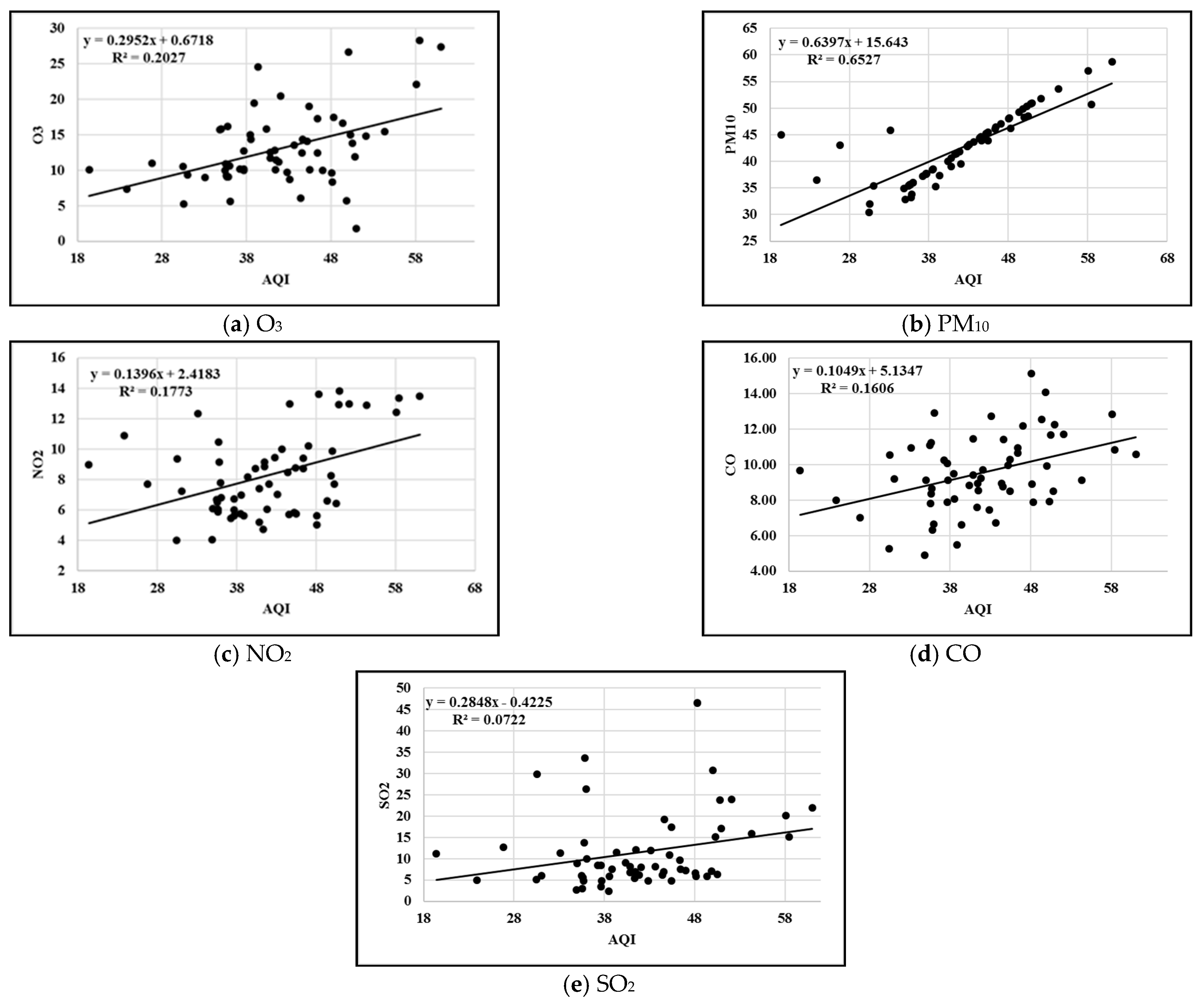
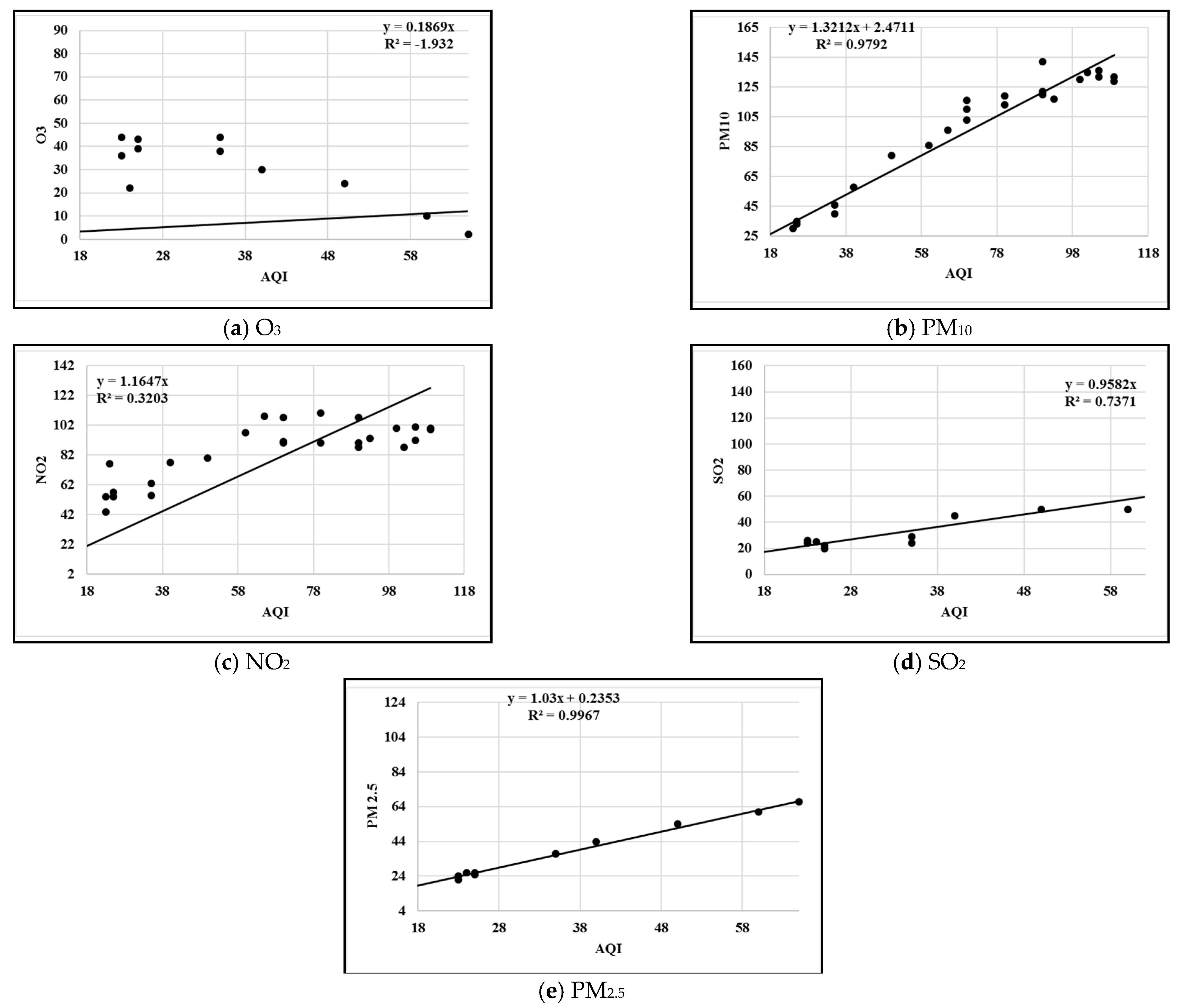
3.4. Correlation Analysis

Correlation analysis is used to quantify the degree of relationship between two continuous variables, such as in between an independent and a dependent variable or between two independent variables. The correlation analysis is meant to prove or validate the correctness of the air pollution risk assessment operation. Figure 7a–e highlights the correlation between AQI reading and the concentrations of the parameters that affect air quality in the Malaysia case study, which are O3, PM10, NO2, CO, and SO2. The figures show that O3, NO2, and CO concentrations are around 0.2, with SO2 having an even lower correlation of 0.08. These concentrations indicate a very low relationship with the AQI reading but will alert the prediction system if the concentrations increase. The highest correlation between the concentrations and the AQI is of PM10, which correlates with around 0.7. This indicates a high presence of particulate matter <10 μm in Malaysian air.
Next, Figure 8a–e highlights the correlation between AQI reading and all parameters that affect air quality in the China case study, which are O3, PM10, NO2, SO2, and PM2.5. From the figures, it can be seen that most of the concentration correlations are higher in China compared to Malaysia. Correlations of O3 and NO2 are low, around 0.2 and 0.3, respectively. Other parameters show a high correlation with AQI in China, with SO2 around 0.6, while PM2.5 and PM10 are both around 0.9.
For both case studies in Malaysia and China, the correlation analysis shows that the particulate matter, which is small enough to be suspended in the air, has a high degree of relationship with the AQI. In general, particle matter less than 10 μm in diameter can get deep into the lungs and, in some cases, into the bloodstream, which must be monitored closely by both countries. This implies that PM2.5, tiny particles in the air that are two and one half microns or less in width, pose the greatest risk to health as compared to PM10. Studies show that ambient PM2.5 concentrations were significantly associated with influenza-like illness (ILI) risk in Beijing, China [11].

4. Results and Discussion

Prediction of the air pollutant concentrations represents a complex spatio-temporal problem due to the dynamic nature and high spatio-temporal variability in air pollution data. This section presents the results of the AQI prediction between three models: (i) the base model ARIMA; (ii) the ANFIS model of Prasad et al. [12]; and (iii) the improved ARI APGRA model by MA-based MCS algorithm. Prediction model performance is evaluated according to accuracy based on MAE and RMSE as well as prediction ability based on the coefficient of determination R2.

4.1. Comparison between AQI Prediction Models

The experiments aim to examine the proposed model effectiveness in predicting AQI concentrations for one day and two days in advance. The results are compared between the real AQI values against the base models of ARIMA, ANFIS, and the APGRA models for two separate case studies from Malaysia and China. Based on Table 3, the best prediction in the Malaysia case study achieved for one-day prediction is at City 10, and two-day prediction is at City 7. The prediction of the first day yields a lower error than the second day since the prediction error for one day in advance is brought into the next day’s prediction. The APGRA model produced the best results compared to the direct approach in the APGRA and ANFIS models for both one-day and two-day predictions. This shows that the APGRA model plays an important role in obtaining good prediction results with approximately 41% improvement on RMSE. This is attributed to incorporating uncertainty into the prediction, which allows for exploiting the repeated sampling of the operation that improves the accuracy of the forecasting. From the aspect of absolute errors, as measured by RMSE and MAE, the best prediction for one day is achieved by City 10 using MCS. The fact that City 10 produced lower absolute error than other cities indicates the importance of the local environment where a station is located. City 10 is located in the zone of “clean source”. Therefore, the low variability of AQI concentrations makes it easier to predict than other cities. Nevertheless, the best R2 is achieved for both one-day and two-day predictions at City 8, which indicates that the relative measure can objectively evaluate the prediction model in different backgrounds. The AQI prediction results showed a good R2. Moreover, ARIMA produced better results than the APGRA model and ANFIS approach for both one-day and two-day prediction in terms of processing time. The result shows that the best algorithm among the three is the APGRA model in terms of RMSE and MAE as it achieves an average R2 of 0.772, RMSE of 1.891, MAE of 1.642 and time of 7.57. The basic ARIMA average is R2 of 0.571, RMSE of 3.22, MAE of 2.874, and time of 5.97. The ANFIS benchmark average R2 of 0.48, RMSE of 3.7, MAE of 3.33 time of 10.37.
Based on Table 4, the best prediction in the China case study is achieved for one-day in City 1, and two-day is at City 3. The prediction values of the first day yield lower error rates than the second day. This can be explained by the theory of error accumulation since the forecasting error for one day in advance is brought into the next day’s prediction. The ARIMA-based MCS yields better results than the direct approach ARIMA and ANFIS models for both one-day and two-day forecasts. This confirms the ability of the Monte Carlo simulation to accurately reproduce the sample, which boosts the predictive power of ARIMA. The results show that the ARIMA-based MCS algorithm plays an important role in obtaining good prediction results with approximately 47% improvement on RMSE. As measured by RMSE and MAE, the best prediction is achieved for one day using the APGRA model from the aspect of absolute error. Nevertheless, the best R2 is achieved for both one-day and two-day predictions, which indicates that the relative measure can evaluate the prediction model in different backgrounds.
Subsequently, the APGRA model provides the best solution among the three in terms of RMSE, MAE, and R2. The model achieves an average R2 of 0.852, RMSE of 7.509, MAE of 5.909, and time of 3.34. The basic ARIMA average R2 of 0.718, RMSE of 14.14, MAE of 11.86, and time of 2.65. The ANFIS benchmark model achieves an average R2 of 0.615, RMSE of 13.426, MAE of 11.4146, and time of 7.7.

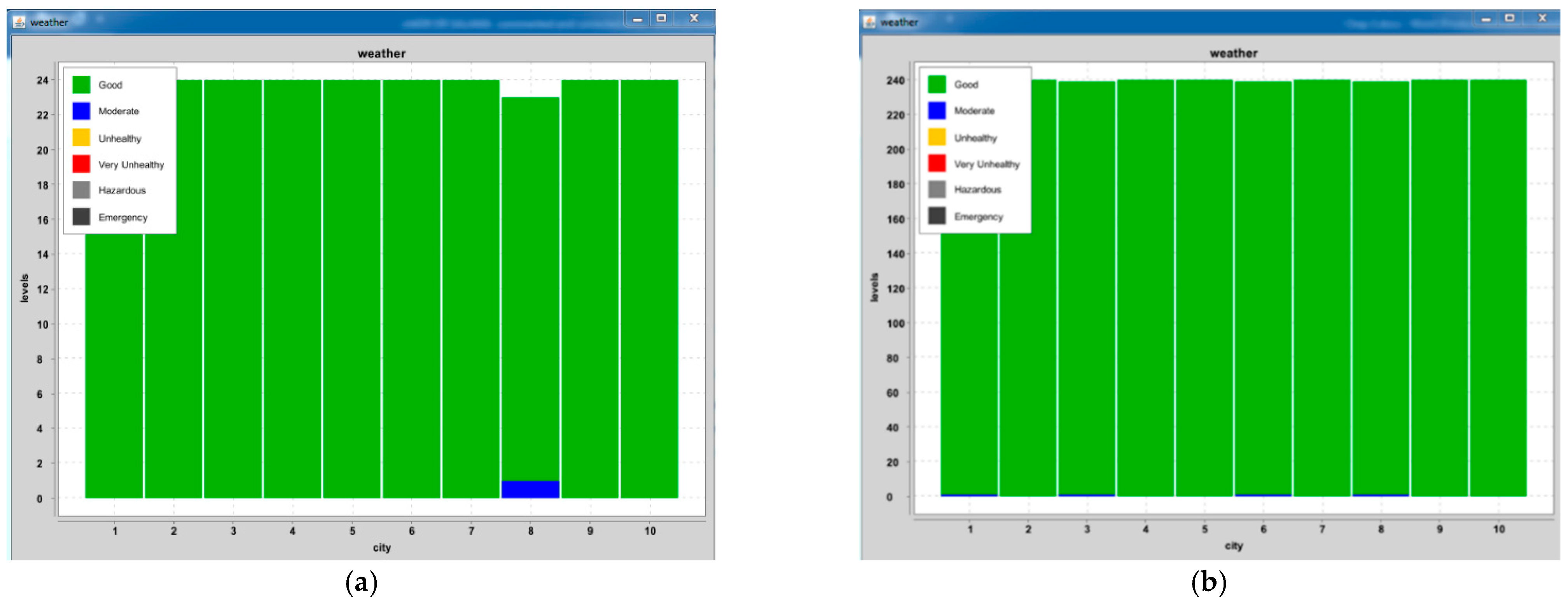
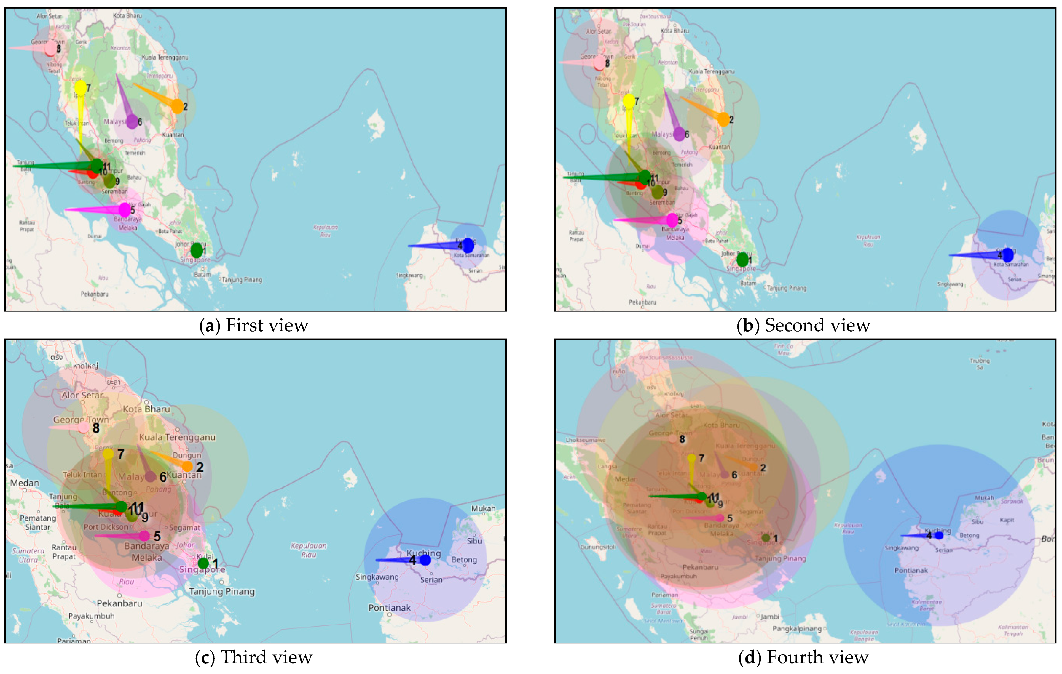
4.2. Results of Global Air Pollution Risk Assessment Model

The APGRA model is the best prediction algorithm because it scores the lowest error from the earlier analysis. However, the AQI’s prediction poses a distributed problem because the pollution risks are distributed in multiple places of cities. In turn, the process of risk as a prediction model is important to aggregate the risks from various local stations as represented in cities in both Malaysia and China case studies. Moreover, finding the risk level from AQI of various parameters is one of the main objectives of this research. As a result, this paper proposes a Global Air Pollution Risk Assessment (APGRA) model based on a collaborative multi-agent architecture where each city is modeled as a collaborative agent. This model, therefore, aggregates risk input from multiple agents residing in distributed cities to produce a single global air pollution prediction value. An APGRA model is implemented in a system for testing and evaluation to achieve this. Figure 9a shows the mediator agent in APGRA with a dynamic selection of the number of agents to work with. The mediator agent in the APGRA model is responsible for decision-making depending on the information that comes from multiple agents (cities). The information that comes from the multi-agents includes the configuration of the main agent, the direction of the wind, the threshold for the error of prediction, the amount of data, the information sent between agents, the main city understudy, and other cities affected by the main city. The main agent aggregates all risk information calculated by the multi-agents depending on the individual AQI level in each city. The parameter of different forms of air pollution in this research depends on the case study. Malaysia, for example, does not measure PM2.5 in all cities. The mediator agent in APGRA monitors and visualizes the current range of data as determined by the user, along with options to filter data by year, month, and day. APGRA also provided the option to choose the model for calculating local AQI prediction, such as the ARIMA-based MCS. This model relies on cooperative multi-agents to produce the global assessment of air pollution. Figure 9b shows the cooperation process among the single agents representing a single city. Assessment becomes more complex and challenging, resulting in a global air pollution risk.
Figure 10a,b show the global AQI values from all cities in the different case studies (Malaysia and China). Note that the proposed ARIMA-based MCS algorithm conducted local prediction of AQI levels. Subsequently, the APGRA model under this multi-agent architecture produces a singular global air pollution risk prediction value.
The APGRA model depends on the wind data, which are wind speed and wind directions, to produce the global prediction value. This is important to illustrate the dynamic changes of air pollution risks for a specific city concerning other cities. Wind direction determines the direction of pollution, while wind speed determines the zone pollution. There exists a direct correlation between the pollution zone and wind speed. When the wind speed increases, the zones of pollution increases as well, and this relationship can be shown by the APGRA. Figure 11 explains how the APGRA model work relies on wind data in several cities in Malaysia with a ring of pollution zone between 0.5 km to 5 km.
Based on Figure 11, if the wind speed is normal at 5 km/h, the zone pollution will be 0.5 km (refer to Figure 11a). If the wind speed is between 10 to 20 km/h, the zone pollution will be 1 km (refer to Figure 11b). If the wind speed is between 20 to 30 km/h, the zone pollution will be 2 km (refer to Figure 11c). Finally, if the wind speed is more than 30 km/h, the zone pollution will be 5 km (refer to Figure 11d).
Table 5 explains the results of the global air pollution risk assessment model that depends on wind data to calculate the interaction pollution among cities for two case studies (Malaysia and China). The proposed model calculates the air pollution level for each city then calculates the global air pollution level for all cities. The wind speed corresponds to the area of pollution zones, whereas the area of pollution zone increases proportionally according to the increase of wind speed. The wind direction responds to the direction of pollution, which might also affect the other cities. The obtained results of the APGRA model are compared with the actual data of the ten cities in both case studies. The estimated risk levels of the 10 cities in both case studies have a full match. This indicates that the APGRA model correctly predicts global risk levels. This is attributed to the ability of APGRA to assess the global value of the AQI and take into account dynamic parameter readings at multiple, distributed local stations. Therefore, the prediction model becomes aware of the global aspect regarding possible interaction between individual cities, which improves the proposed APGRA.
Table 5 appointed the RMSE, MAE, R2, and processing time. The APGRA model matches greatly with actual data, representing R2, that showed low errors, good processing time, good ability, and flexibility. At the same time, the Malaysia case study’s average performance metrics are R2 of 0.7, RMSE of 2.064, MAE of 1.32, and time of 4.11. Likewise, China’s case study average performance metrics are R2 of 0.73, RMSE of 4.72, MAE of 3.385, and a time of 3.36.

5. Conclusions

This paper proposed a new air pollution global risk assessment (APGRA) model for predicting spatial correlation AQI risk assessment to address these issues. The APGRA model incorporates the autoregressive integrated moving average (ARIMA), Monte Carlo simulation (MCS), the collaborative multi-agent system (MAS), and the prediction algorithm for reducing AQI prediction error and time. The proposed APGRA model was evaluated based on Malaysia and China’s two real-world air quality datasets. The APGRA model improved the average Root Mean Squared Error (RMSE) by 41%, and the Mean and Absolute Error (MAE) by 47.10% when compared to the conventional ARIMA model and ANFIS model. The accuracy level of the ARIMA-based MCS algorithm was stably higher than that of ARIMA. In particular, RMSE and MAE of ARIMA-based MCS algorithm generated significant improvements, which helps to estimate the variation trend of the AQI concentrations. The proposed model provided the variance prediction in addition to AQI concentrations prediction, expressing more information on the forecasting target. We analyzed and explained the AQI concentrations prediction with the ARIMA-based MCS algorithm, and the simulation results proved outstanding in adapting to the proposed model. The ARIMA-based MCS algorithm can be applied to other AQI forecasting if the model’s appropriate input variables are selected. Some issues still need further investigation. This includes study areas that their PM2.5 emission data was not available. The PM2.5 with complex components exhibits a high correlation with the other AQIs. It is rather remarkable that the influence of PM2.5 on AQI should be considered in the forecasting system. The PM2.5 with complex components is another issue that exhibits a high correlation with the other AQIs. Therefore, it is rather remarkable that the influence of different AQIs on PM2.5 should be considered in the forecasting system. As we mentioned before, the APGRA model solves the global pollution interaction between cities depending on a local ARIMA-based MCS algorithm developed in this paper and some additional parameters such as wind speed and wind direction. The issue with the ARIMA-based MCS algorithm is the cost of the simulation, resulting from the need to apply significant values of p and q that led to consuming processing time.

Author Contributions

Conceptualization, M.H.H. and S.A.M.; methodology, M.H.H., S.A.M. and A.M.; software, M.H.H. and M.A.J.; validation, M.H.H., S.A.M. and M.Z.S.; formal analysis, M.H.H. and B.A.S.A.-r.; investigation, M.H.H. and S.A.M.; resources, M.Z.S., F.S. and A.E.M.E.; data curation, M.H.H.; writing—original draft preparation, M.H.H., S.A.M. and A.M.; writing—review and editing, M.H.H., S.A.M. and M.A.J.; visualization, M.H.H., F.S. and B.A.S.A.-r.; supervision, S.A.M. and A.M.; project administration, M.Z.S., S.A.M. and A.M.; funding acquisition, M.Z.S., S.A.M. and A.E.M.E. All authors have read and agreed to the published version of the manuscript.

Funding

The authors express appreciation to the Malaysia Ministry of Higher Education (MoHE). This research was funded by the Fundamental Research Grant Scheme (FRGS/1/2019/ICT04/UTHM/03/1) grant vot number K209.

Informed Consent Statement

Not applicable.

Data Availability Statement

The used dataset of this research is available online and has a proper citation within the paper contents.

Acknowledgments

The authors would like to thank the Department of Environment (DOE) for providing the required data and assistance for this work. The authors also would like to thank the Center of Intelligent and Autonomous Systems (CIAS) at the Faculty of Computer Science and Information Technology (FSKTM), Universiti Tun Hussein Onn Malaysia (UTHM) for supporting this work.

Conflicts of Interest

The authors declare that they have no conflict of interest to be addressed related to this work.

References

  1. Zhang, S.; Guo, B.; Dong, A.; He, J.; Xu, Z.; Chen, S.X. Cautionary tales on air-quality improvement in Beijing. Proc. R. Soc. A Math. Phys. Eng. Sci. 2017, 473, 20170457. [Google Scholar] [CrossRef] [PubMed] [Green Version]
  2. Liu, Y.S.; Cao, Y.; Hou, J.J.; Zhang, J.T.; Yang, Y.O.; Liu, L.C. Identifying common paths of CO2 and air pollutants emissions in China. J. Clean. Prod. 2020, 256, 120599. [Google Scholar] [CrossRef]
  3. Li, J.; Tartarini, F. Changes in air quality during the COVID-19 lockdown in Singapore and associations with human mobility trends. Aerosol Air Qual. Res. 2020, 20, 1748–1758. [Google Scholar] [CrossRef]
  4. Nyoni, T.; Mutongi, C. Modeling and forecasting carbon dioxide emissions in China using Autoregressive Integrated Moving Average (ARIMA) models. EPRA Int. J. Multidiscip. Res. 2019, 5, 215–224. [Google Scholar]
  5. Bakhtavar, E.; Hosseini, S.; Hewage, K.; Sadiq, R. Air pollution risk assessment using a hybrid fuzzy intelligent probability-based approach: Mine blasting dust impacts. Nat. Resour. Res. 2021, 30, 2607–2627. [Google Scholar] [CrossRef]
  6. Siwek, K.; Osowski, S. Data mining methods for prediction of air pollution. Int. J. Appl. Math. Comput. Sci. 2016, 26, 467–478. [Google Scholar] [CrossRef] [Green Version]
  7. Yang, Z.; Wang, J. A new air quality monitoring and early warning system: Air quality assessment and air pollutant concentration prediction. Environ. Res. 2017, 158, 105–117. [Google Scholar] [CrossRef]
  8. Tong, R.; Cheng, M.; Zhang, L.; Liu, M.; Yang, X.; Li, X.; Yin, W. The construction dust-induced occupational health risk using Monte-Carlo simulation. J. Clean. Prod. 2018, 184, 598–608. [Google Scholar] [CrossRef]
  9. Song, C.; Fu, X. Research on different weight combination in air quality forecasting models. J. Clean. Prod. 2020, 261, 121169. [Google Scholar] [CrossRef]
  10. Yang, H.; O’Connell, J.F. Short-term carbon emissions forecast for aviation industry in Shanghai. J. Clean. Prod. 2020, 275, 122734. [Google Scholar] [CrossRef]
  11. Feng, X.; Li, Q.; Zhu, Y.; Hou, J.; Jin, L.; Wang, J. Artificial neural networks forecasting of PM2.5 pollution using air mass trajectory based geographic model and wavelet transformation. Atmos. Environ. 2015, 107, 118–128. [Google Scholar] [CrossRef]
  12. Prasad, K.; Gorai, A.K.; Goyal, P. Development of ANFIS models for air quality forecasting and input optimization for reducing the computational cost and time. Atmos. Environ. 2016, 128, 246–262. [Google Scholar] [CrossRef]
  13. Zio, E. Challenges in the vulnerability and risk analysis of critical infrastructures. Reliab. Eng. Syst. Saf. 2016, 152, 137–150. [Google Scholar] [CrossRef]
  14. Wang, P.; Zhang, H.; Qin, Z.; Zhang, G. A novel hybrid-Garch model based on ARIMA and SVM for PM2. 5 concentrations forecasting. Atmos. Pollut. Res. 2017, 8, 850–860. [Google Scholar] [CrossRef]
  15. Hernandez-Matamoros, A.; Fujita, H.; Hayashi, T.; Perez-Meana, H. Forecasting of COVID19 per regions using ARIMA models and polynomial functions. Appl. Soft Comput. 2020, 96, 106610. [Google Scholar] [CrossRef] [PubMed]
  16. Benvenuto, D.; Giovanetti, M.; Vassallo, L.; Angeletti, S.; Ciccozzi, M. Application of the ARIMA model on the COVID-2019 epidemic dataset. Data Brief 2020, 29, 105340. [Google Scholar] [CrossRef] [PubMed]
  17. Westerlund, J.; Urbain, J.P.; Bonilla, J. Application of air quality combination forecasting to Bogota. Atmos. Environ. 2014, 89, 22–28. [Google Scholar] [CrossRef]
  18. Mannshardt, E.; Benedict, K.; Jenkins, S.; Keating, M.; Mintz, D.; Stone, S.; Wayland, R. Analysis of short-term ozone and PM2. 5 measurements: Characteristics and relationships for air sensor messaging. J. Air Waste Manag. Assoc. 2017, 67, 462–474. [Google Scholar] [CrossRef] [PubMed] [Green Version]
  19. Qazi, A.; Shamayleh, A.; El-Sayegh, S.; Formaneck, S. Prioritizing risks in sustainable construction projects using a risk matrix-based Monte Carlo Simulation approach. Sustain. Cities Soc. 2021, 65, 102576. [Google Scholar] [CrossRef]
  20. Zhao, L.; Ji, Y.; Yao, J.; Long, S.; Li, D.; Yang, Y. Quantifying the fate and risk assessment of different antibiotics during wastewater treatment using a Monte Carlo simulation. J. Clean. Prod. 2017, 168, 626–631. [Google Scholar] [CrossRef]
  21. Gordy, M.B.; Juneja, S. Nested simulation in portfolio risk measurement. Manag. Sci. 2010, 56, 1833–1848. [Google Scholar] [CrossRef] [Green Version]
  22. Mostafa, S.A.; Ahmad, M.S.; Annamalai, M.; Ahmad, A.; Gunasekaran, S.S. A dynamically adjustable autonomic agent framework. In Advances in Information Systems and Technologies; Springer: Berlin/Heidelberg, Germany, 2013; pp. 631–642. [Google Scholar]
  23. Hassan, M.H.; Mostafa, S.A.; Mustapha, A.; Abd Wahab, M.H.; Nor, D.M. A survey of multi-agent system approach in risk assessment. In Proceedings of the 2018 International Symposium on Agent, Multi-Agent Systems and Robotics (ISAMSR), Putrajaya, Malaysia, 27–28 August 2018; Institute of Electrical and Electronics Engineers (IEEE): Putrajaya, Malaysia, 2018; pp. 1–6. [Google Scholar]
  24. Mostafa, S.A.; Ahmad, M.S.; Ahmad, A.; Annamalai, M. Formulating situation awareness for multi-agent systems. In Proceedings of the 2013 International Conference on Advanced Computer Science Applications and Technologies, Kuching, Malaysia, 23–24 December 2013; Institute of Electrical and Electronics Engineers (IEEE): Kuching, Malaysia, 2013; pp. 48–53. [Google Scholar]
  25. Kashinath, S.A.; Mostafa, S.A.; Mustapha, A.; Mahdin, H.; Lim, D.; Mahmoud, M.A.; Yang, T.J. Review of data fusion methods for real-time and multi-sensor traffic flow analysis. IEEE Access 2021, 9, 51258–51276. [Google Scholar] [CrossRef]
  26. Mostafa, S.A.; Hazeem, A.A.; Khaleefahand, S.H.; Mustapha, A.; Darman, R. A collaborative multi-agent system for oil palm pests and diseases global situation awareness. In Proceedings of the Future Technologies Conference, Vancouver, BC, Canada, 13–14 November 2018; Springer: Cham, Switzerland, 2018; pp. 763–775. [Google Scholar]
  27. Mostafa, S.A.; Mustapha, A.; Gunasekaran, S.S.; Ahmad, M.S.; Mohammed, M.A.; Parwekar, P.; Kadry, S. An agent architecture for autonomous UAV flight control in object classification and recognition missions. Soft Comput. 2021, 1–14. [Google Scholar] [CrossRef]
  28. Khalaf, B.A.; Mostafa, S.A.; Mustapha, A.; Mohammed, M.A.; Mahmoud, M.A.; Al-Rimy, B.A.S.; Marks, A. An Adaptive Protection of Flooding Attacks Model for Complex Network Environments. Secur. Commun. Netw. 2021, 2021. [Google Scholar] [CrossRef]
  29. Mostafa, S.A.; Gunasekaran, S.S.; Ahmad, M.S.; Ahmad, A.; Annamalai, M.; Mustapha, A. Defining tasks and actions complexity-levels via their deliberation intensity measures in the layered adjustable autonomy model. In Proceedings of the 2014 International Conference on Intelligent Environments (IE ’14), Shanghai, China, 30 June–4 July 2014; Institute of Electrical and Electronics Engineers (IEEE): Shanghai, China, 2014; pp. 52–55. [Google Scholar]
  30. Mostafa, S.A.; Mustapha, A.; Mohammed, M.A.; Ahmad, M.S.; Mahmoud, M.A. A fuzzy logic control in adjustable autonomy of a multi-agent system for an automated elderly movement monitoring application. Int. J. Med. Inform. 2018, 112, 173–184. [Google Scholar] [CrossRef] [PubMed]
  31. Bellifemine, F.L.; Caire, G.; Greenwood, D. Developing Multi-Agent Systems with JADE; John Wiley & Sons: Chichester, UK, 2007. [Google Scholar]
Figure 1. The geographic position of the Malaysia case study.
Sustainability 14 00510 g001
Figure 2. The geographic position of the China air pollution case study [1].
Sustainability 14 00510 g002
Figure 3. The asynchronous message passing in a MAS [31].
Sustainability 14 00510 g003
Figure 4. A single agent processing cycle.
Sustainability 14 00510 g004
Figure 5. Air Pollution Global Risk Assessment (APGRA) model.
Sustainability 14 00510 g005
Figure 6. An example application of the APGRA model.
Sustainability 14 00510 g006
Figure 7. Correlation between AQI levels and all parameters in Malaysia.
Sustainability 14 00510 g007
Figure 8. Correlation between AQI levels and all parameters in China.
Sustainability 14 00510 g008
Figure 9. The implementation results of the APGRA model. (a) The GUI of the mediator agent; (b) Cooperation among agents.
Sustainability 14 00510 g009
Figure 10. The AQI levels of different cities.(a) Global AQI level in Malaysia dataset; (b) Global AQI levels in China dataset.
Sustainability 14 00510 g010
Figure 11. The radius of pollution.
Sustainability 14 00510 g011
Table 1. Area of air quality data in Malaysia.
NOSite StateSite IDLocationLatitudeLongitudeType
1JohorCAS 001SM Pasir Gudang 2, Pasir Gudang, JohorN01° 28.225E103° 53.637Residential
2TerengganuCAE 002SRK Bukit Kuang, Teluk Kalung, Kemaman.N04° 16.260E103° 25.826Residential
3Pulau PinangCAN 003Sek. Keb. Cenderawasih, Tmn. Inderawasih, PeraiN05° 23.470E100° 23.213Residential
4SarawakCAK 004Medical Store, Kuching, SarawakN01° 33.734E110° 23.329Residential
5MelakaCAS 006Sek. Men. Keb. Bukit Rambai, MelakaN02° 15.510E102° 10.364Residential
6PahangCAE 007Pej. Kajicuaca, Batu Embun, Jerantut, PahangN03° 58.238E102° 20.863Residential
7PerakCAN 008SM Jalan Tasek, Ipoh, PerakN04° 37.781E101° 06.964Residential
8Pulau PinangCAN 009SK Seberang Jaya II, Perai, Pulau PinangN05° 23.890E100° 24.194Residential
9Negeri SembilanCAC 010Taman Semarak (Phase II), Nilai, N.SembilanN02° 49.246E101° 48.877Residential
10SelangorCAC 011SM(P) Raja Zarina, Klang, SelangorN03° 00.620E101° 24.484Residential
Table 2. Area of air quality data in China.
Dataset CharacteristicsMultivariate, Time-Series
Number of Instances:420,768
Area:Physical
Number of Attributes:18
Attribute Characteristics:Integer, Real
Missing Values?Yes
Associated Tasks:Regression
Table 3. Comparison between the three AQI prediction algorithms in Malaysia dataset.
AQI 1-Day Advance Prediction
MetricCity 1City 2City 3City 4City 5City 6City 7City 8City 9City 10
ARIMAR20.830.240.330.470.870.340.480.920.890.34
RMSE3.842.834.992.663.782.772.183.114.711.33
MAE3.452.694.402.323.402.262.042.784.301.10
Time7.206.305.206.306.504.703.806.606.906.20
MCSR20.910.750.500.640.890.880.730.940.920.56
RMSE2.151.082.051.243.081.921.022.473.100.80
MAE1.901.031.891.062.601.600.882.112.700.65
Time8.408.306.208.307.506.706.807.507.908.10
ANFISR20.80.60.40.30.80.10.10.90.70.1
RMSE4.33.353.24.542.33.452
MAE43.14.42.74.13.5234.81.7
Time10.4012.30911999111211
AQI 2-Day Advance Prediction
MetricCity 1City 2City 3City 4City 5City 6City 7City 8City 9City10
ARIMAR20.120.200.300.390.010.020.250.820.800.10
RMSE19.409.205.9022.3014.808.103.606.7612.6016.20
MAE15.307.205.3116.8012.006.903.363.8010.5011.38
Time9.207.407.207.307.506.706.808.808.307.30
MCSR20.200.500.400.400.890.080.750.900.880.49
RMSE10.905.364.5211.304.472.501.724.149.004.60
MAE7.963.753.778.513.541.951.422.667.002.80
Time9.809.409.809.509.208.708.309.809.309.30
ANFISR20.10.40.60.40.10.10.30.90.80.2
RMSE199.33.9221482.73.21216.4
MAE15.67.43.3171272.32.91011.7
Time13151415141314151514
Table 4. Comparison between the three AQI prediction algorithms in China dataset.
AQI 1-Day Advance Prediction
MetricCity 1City 2City 3City 4City 5City 6City 7City 8City 9City 10
ARIMAR20.970.940.550.890.580.450.660.400.810.93
RMSE4.459.786.1410.05.4620.221.430.419.114.24
MAE3.328.395.388.544.8815.116.726.317.412.46
Time2.703.002.502.802.302.702.702.802.902.10
MCSR20.980.950.830.910.730.810.930.500.910.97
RMSE2.704.642.955.702.3016.79.8011.012.96.40
MAE1.803.752.404.542.0011.77.109.8010.75.30
Time3.103.903.103.903.103.103.903.103.103.10
ANFISR20.80.80.400.790.630.250.690.140.730.92
RMSE4.4310.36.098.996.1213.319.730.020.514.7
MAE3.228.65.17.95.4110.815.92618.312.9
Time7878878987
AQI 2-Day Advance Prediction
MetricCity 1City 2City 3City 4City 5City 6City 7City 8City 9City 10
ARIMAR20.900.860.690.640.890.740.520.300.580.817
RMSE15.822.111.115.013.230.325.238.721.618.98
MAE9.9117.28.4211.19.3825.621.530.320.116.25
Time3.204.104.104.104.303.203.203.204.304.30
MCSR20.940.870.760.750.960.850.820.400.810.90
RMSE11.615.77.2011.29.7021.915.027.013.711.50
MAE6.8010.64.707.406.0017.911.817.012.19.00
Time4.104.904.804.904.804.804.804.104.804.10
ANFISR20.90.80.50.60.80.70.50.50.50.8
RMSE1622111513.53024392319
MAE10178119.52621302016
Time99889.209.309.209.408.908.60
Table 5. Sample of global air pollution risk levels.
AQI 1-Day Advance Assessment of Risk Level in Malaysia Dataset
ResultsCity 1City 2City 3City 4City 5City 6City 7City 8City 9City 10
Risk levelgoodgoodmoderategoodgoodgoodgoodmoderate moderate good
Affected bynonenone7,9none3,8nonenone7,9none9
Effect onnonenone5nonenonenone357,3,10none
Effect zone120.5110.52221
R20.90.60.50.80.70.60.60.70.80.6
RMSE1.062.62.981.71.822.23.11.31.9
MAE0.71.21.71.21.371.51.551.780.91.3
Time3.205.304.203.303.204.904.803.203.905.10
AQI 1-Day Advance Assessment of Risk Level in China Dataset
ResultsCity 1City 2City 3City 4City 5City 6City 7City 8City 9City 10
Risk levelmoderategoodmoderategoodgoodmoderategoodmoderategoodgood
Affected bynone94nonenonenonenone4none4
Effect on nonenonenone8,3,10nonenonenonenone2none
Effect zone0.50.5110.50.50.520.50.5
R20.60.60.80.80.90.50.70.70.80.9
RMSE2.83.24.555.25.14.85.86.84
MAE2.12.43.23.754.13.63.444.52.8
Time3.703.203.103.203.203.203.203.703.903.20
Publisher’s Note: MDPI stays neutral with regard to jurisdictional claims in published maps and institutional affiliations.

