Toward Baggage-Free Airport Terminals: A Case Study of London City Airport

Abstract

Nowadays, the aviation industry pays more attention to emission reduction toward the net-zero carbon goals. However, the volume of global passengers and baggage is exponentially increasing, which leads to challenges for sustainable airports. A baggage-free airport terminal is considered a potential solution in solving this issue. Removing the baggage operation away from the passenger terminals will reduce workload for airport operators and promote passengers to use public transport to airport terminals. As a result, it will bring a significant impact on energy and the environment, leading to a reduction of fuel consumption and mitigation of carbon emission. This paper studies a baggage collection network design problem using vehicle routing strategies and augmented reality for baggage-free airport terminals. We use a spreadsheet solver tool, based on the integration of the modified Clark and Wright savings heuristic and density-based clustering algorithm, for optimizing the location of logistic hubs and planning the vehicle routes for baggage collection. This tool is applied for the case study at London City Airport to analyze the impacts of the strategies on carbon emission quantitatively. The result indicates that the proposed baggage collection network can significantly reduce 290.10 tonnes of carbon emissions annually.

1. Introduction

The International Air Transport Association (IATA) [1] predicts that over 10 billion air passengers will be carried by 2050 (approximately traveling 20 trillion kilometers each year), which will generate about 1800 megatonnes (Mt) of carbon emissions and lead to challenges of passenger and baggage flow management at airport terminals. The aviation industry has embraced this challenge and a wide range of measures are now being implemented to solve the issue toward the net-zero carbon goals. The baggage-free airport terminal (BFAT) is considered a potential solution for the goal of sustainable airports. The BFAT builds new links between airports and cities, investigating the expansion of the baggage collection from home. In particular, the BFAT removes the baggage operation away from the passenger terminal via multiple injection points connected to highly efficient baggage fulfillment centers [2]. The service will pick up passengers’ baggage at a selected time window on the doorstep, assign a QR code to each baggage and deliver the baggage to the assigned depot (logistic hub or airport). Passengers will be encouraged to use public transport during their journey; in the meantime, baggage will be delivered directly to the destination (home or hotel address). Augmented reality (AR) will be used to help passengers quickly double-check their baggage to avoid any mishandling. Hence, the BFAT effectively manages the baggage flow between the airports and the cities, liberating the passengers from their baggage and reducing airport-related carbon emissions.

The location-routing problem (LRP) is one of the main tasks of the BFAT, identifying the optimal location of logistic hubs and planning the optimal vehicle routes for baggage collection and delivery. For a comprehensive literature review of recent research on LRP we refer to [3]. Since the location of logistic hubs will be specified in our study, we focus on solving the vehicle routing problem (VRP). The VRP includes a growing number of variants, such as time windows [4], multiple depots [5], multiple trips [6], heterogeneous fleets [7], and green vehicles [8]. The green vehicle routing problem (GVRP) investigates the negative environmental effects of vehicle transportation. The GVRP expands the traditional VRP’s objective function, in addition to transportation distance, transportation time, and other transportation economic costs, transportation environment cost (e.g., greenhouse gas emissions) is also considered. Bektaş et al. [9] first set carbon emissions as the objective function of VRP. Franceschetti et al. [10] established a GVRP model with time windows to avoid traffic congestion and significantly reduce carbon emissions. Koç et al. [11] found that a fleet with different types of vehicles can reduce pollutant emissions during transport. Zhang et al. [12] developed a two-stage ant colony system (TSACS) to minimize the total carbon emissions on GVRP. Ge et al. [13] introduced the objective functions of cost-saving, energy-saving, and low-carbon cost to the traditional VRP models. The authors designed an improved genetic algorithm for solving this problem. They compared the low-carbon routing with the shortest routing and found that despite the increase in mileage, the carbon emissions have been greatly reduced. The research on the electric vehicle routing problem (EVRP) is a further expansion of the VRP problem [14]. Compared with traditional fossil fuel-powered cars, electric vehicles (EVs) emit fewer greenhouse gas emissions. However, EVs have technical bottlenecks such as smaller transportation coverage and fewer energy replenishment stations. Erdoğan and Miller-Hooks [8] considered EVs into the GVRP models by adding the energy supplement facilities and vehicle travel distance constraints. They provided an effective routing method for EV companies. Felipe et al. [15] proposed the routing problem of electric freight vehicle transportation, considering the time and the charge amount of each EV charging. Schneider et al. [16] developed a new hybrid heuristic algorithm for the electric freight vehicle routing problem with a time window. Omidvar et al. [17] studied additional constraints such as vehicle load and congestion management and incorporated various metaheuristic methods into their solution. According to the International Energy Agency (IEA) [18], a significant number of EVs (around 125 million) will be on the road by 2030. Using EVs for baggage collection and delivery in the BFAT will thus be a future trend. It will be essential to seek solutions for the BFAT toward a sustainable airport industry.

This paper focuses on the VRP with the specified location of logistic hubs for the BFAT’s baggage collection service. The aim is to build a decision support tool for the implementation of a baggage collection service network in airport transportation. This paper discusses the design of an optimal baggage collection network, including the selection of the logistic hub locations and the optimal vehicle routes for baggage collection. A spreadsheet solver tool, based on the integration of the modified Clark and Wright savings heuristic and density-based clustering algorithm, is adopted to find the optimal vehicle routes under different scenarios. For the case study at the London City Airport (LCY), the costs and carbon emissions of using a single depot or multiple depots are investigated and compared. An AR-based innovation is proposed to improve the efficiency of traditional logistics. In summary, this paper makes the following contributions: (i) study a baggage collection service network design problem for future BFATs; (ii) adopt a spreadsheet solver tool to find the optimal vehicle routes for baggage collection; (iii) propose an AR-based baggage tag visualization application, which is useful to reduce any mishandling; (iv) apply the model for the case study at the LCY.

The remainder of the paper is organized as follows: Section 2 describes a spreadsheet solver tool for solving the studied VRP. The case study at the LCY is presented in Section 3. Section 4 is the quantitative analysis of the carbon emissions reduction for the LCY. The AR-based application for baggage tag visualization is presented in Section 5. Lastly, the conclusion and future work are given in Section 6.

2. VRP Spreadsheet Solver Tool

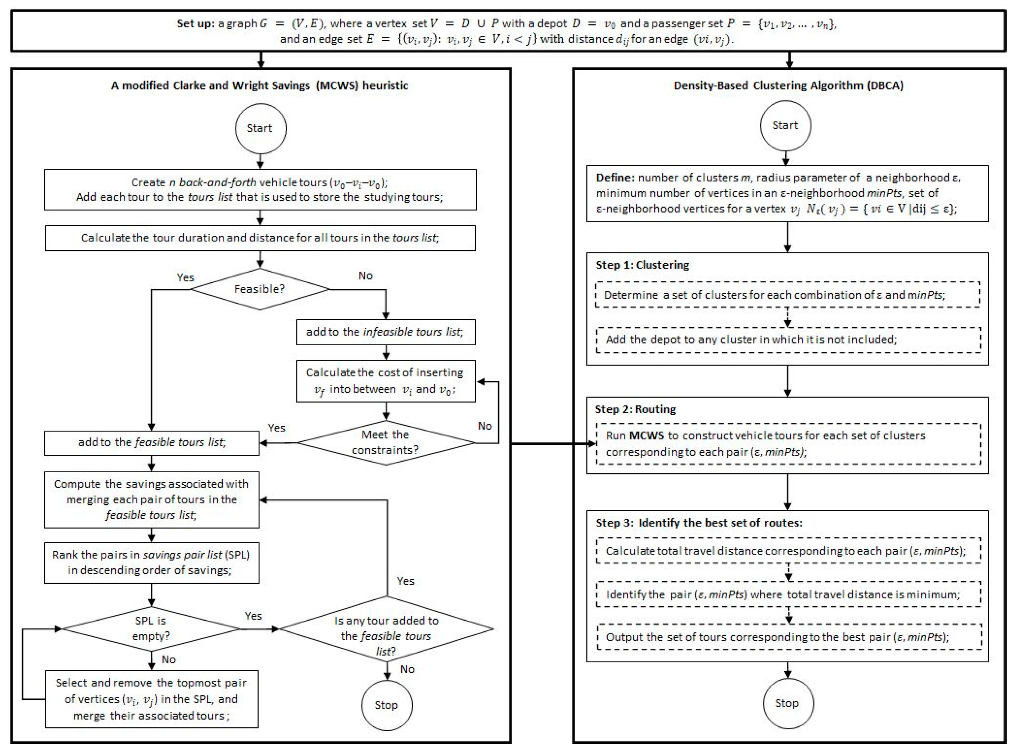
This paper studies the GVRP with a homogeneous fleet of EVs for the BFATs. A spreadsheet solver tool [8] is adopted to solve the GVRP under various scenarios. The solver is developed on the integration of the Modified Clarke and Wright Savings (MCWS) heuristic and the density-based clustering algorithm (DBCA). The MCWS heuristic is applied to construct vehicle tours for each set of clusters in the DBCA’s routing step. The overall aim is to seek a total minimum travel distance for a fleet of EVs that start at a depot, visit a set of customers exactly once, collect their baggage, and return to the depot. A flowchart of the integrated algorithm for the GVRP is shown in Figure 1.

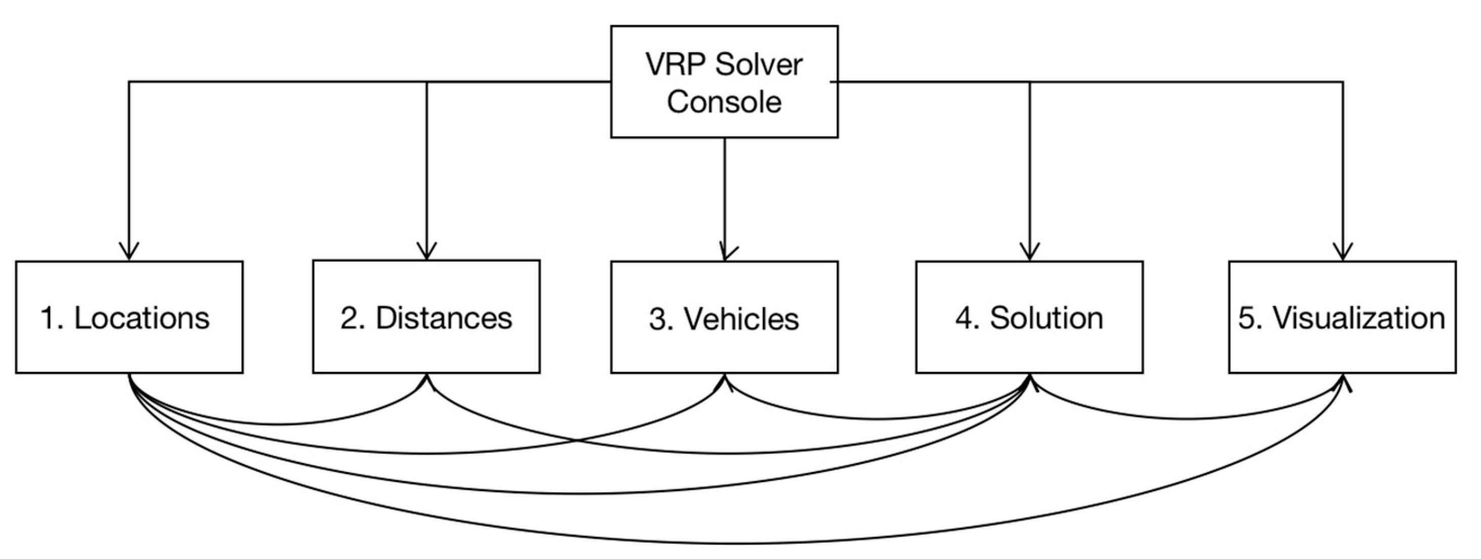
The tool has a unified graphical user interface platform to support users easily to input the data, output the result and visualize the solution. It includes geographic information system (GIS) facilities that allow users to incorporate driving times and distances. The structure of this tool (Locations—Distances—Vehicles—Solution—Visualization) is shown in Figure 2.

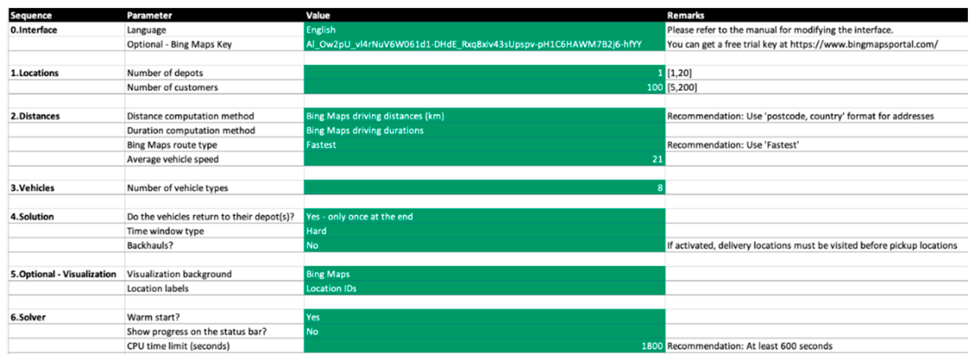
The console spreadsheet breaks down each sequence and provides essential information for each upcoming stage as shown in Figure 3. Users can run the GVRP model with the following six sequences:

-

Sequence 0 (Interface): Retrieve GIS data and establish delivery points for the later sequence.

-

Sequence 1 (Locations): Define the number of depots (e.g., 1–20) and the volume of passengers (e.g., 5–200).

-

Sequence 2 (Distances): Set computation method of distance and driving duration, including Euclidian distances, rounded Euclidian distances, Hamming (Manhattan) distances, Bird’s flight distances, and Bing Maps driving distances.

-

Sequence 3 (Vehicles): Input the number of homogeneous vehicles for simulation (e.g., 8).

-

Sequence 4 (Solution): Set vehicles returning mode and time window type.

-

Sequence 5 (Visualization): Provide visual representation to users, including visualization maps, location IDs, location names, service time, pickup amount, and delivery amount.

-

Sequence 6 (Solver): Start simulation, show progress and result.

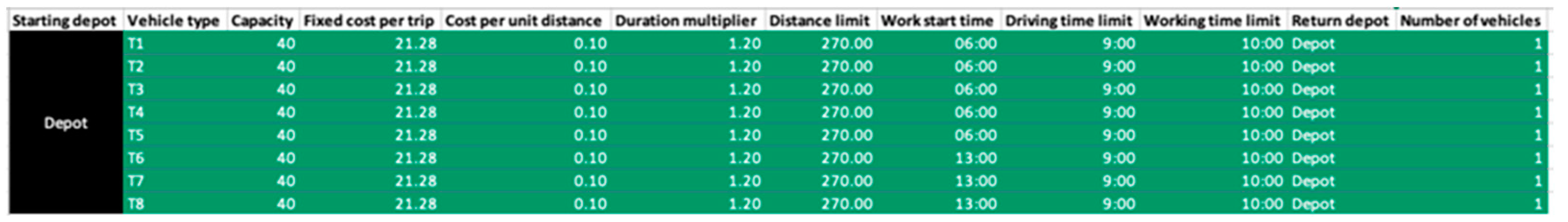
The locations spreadsheet includes passengers’ postcodes, time windows, and pickup amount data from the Civil Aviation Authority (CAA), and the subsequent GIS data (longitude and latitude) from Bing Maps (Figure 4). The distances spreadsheet (Figure 5) calculates the distance and driving duration between every two positions stated in the locations spreadsheet. The vehicles spreadsheet lists different attributes, parameters, and working scenarios. Each vehicle has approximately 14 m³ storage capacity with a standard size of baggage and an 80% capacity utilization rate [19]. The duration multiplier refers to the return driving times for an average-sized vehicle. With the increase in size, speed, and the number of baggage, the duration multiplier is increased by 20%. To keep EV batteries recycled, the distance limit is set to 270 km (80% driving range), as shown in Figure 6. The solution spreadsheet shows passenger-driver solutions based on ‘Locations, Distances, Vehicles’ spreadsheets (Figure 7). The visualization spreadsheet shows the customer locations and vehicle routes with a scatter graph (Figure 8).

3. A Case Study of the London City Airport

The LCY is chosen to validate the model since it is the closest airport to Central London and manages a large number of passengers. In 2019, the LCY handled about 5 million passengers. The CAA shows that 91.8% of the LCY’s passengers depart from the Greater London area [20] (see

Table 1. Passenger distribution for the LCY.

Region	County	Total		County	Total
		000′s	%		000′s	%
South East	Berkshire County	32	0.7	Isle of Wight	0	0.0
	Buckinghamshire County	28	0.6	Kent County	169	3.8
	East Sussex County	21	0.5	Oxfordshire County	19	0.4
	Greater London	4120	91.8	Surrey County	49	1.1
	Hampshire County	30	0.7	West Sussex County	19	0.4
Total	000′s	4487		%	100.0

). In the 2019 Departing Passenger Survey conducted by the CAA, nearly 56% of passengers used private cars to travel to airports, while 44% of passengers used public transport. Private cars emit more greenhouse gases per passenger mile than trains and coaches. Hence, one of the main sources of airport-related emissions is using airport approach roads. Decarbonizing road transport systems to airports has posed challenges to the UK Department of Transport.

In the case study, we focus on a baggage collection service network design from passengers’ sources to the LCY that aims to mitigate the burden of baggage management from passengers and at the airport’s check-in process. The mitigation can encourage passengers to use more public transport to the LCY and reduce airport-related carbon emissions. A similar planning model can be extended for the baggage delivery problem from the airport to the passengers’ destination (home or hotel address).

In the case study, two design scenarios are considered and compared, i.e., one hub at the LCY and multiple logistic hubs in Greater London. In the first scenario (i.e., one hub at the LCY), passengers book baggage collection online, then the entire baggage check-in process happens on the doorstep, finally, the EVs transport all the collected baggage directly to the LCY. In the second scenario (i.e., multiple logistic hubs in Greater London), passengers can bring their baggage to the nearest logistic hub by themselves or can book baggage collection online. Different from the first scenario, the second one aims to deliver the collected baggage to the nearest logistics hub, then unload the baggage from EVs, and finally transport them to the LCY together [21]. In this paper, we compare the transportation distance, transportation cost, and carbon emissions of the solutions for these two scenarios. The spreadsheet solver tool is used to optimize the scenarios and visualize the solutions. The following are assumptions and data of the case study:

-

A one-to-one service between each EV and passengers without repeat.

-

Randomly generate passengers’ location and the number of baggage.

-

A total of 100 passengers book this baggage collection service.

-

Maximum 30 bags in each EV.

-

A 20 miles per hour of average vehicle speed.

-

The range of EVs is up to 211 miles, an ‘Arrival van’ costs GBP 37.24 to charge 80% [22].

-

Driver’s working hour is limited to be 8 h [23].

-

The on-doorstep check-in takes an average of 5 min per baggage, including scan, record, encapsulating, and loading baggage.

-

24 h service with three shifts: 8 a.m., 4 p.m., and 12 p.m.

-

Bing Maps driving distances are used for calculating Evs’ driving distances.

-

The EV will only return to the depot after completing their route.

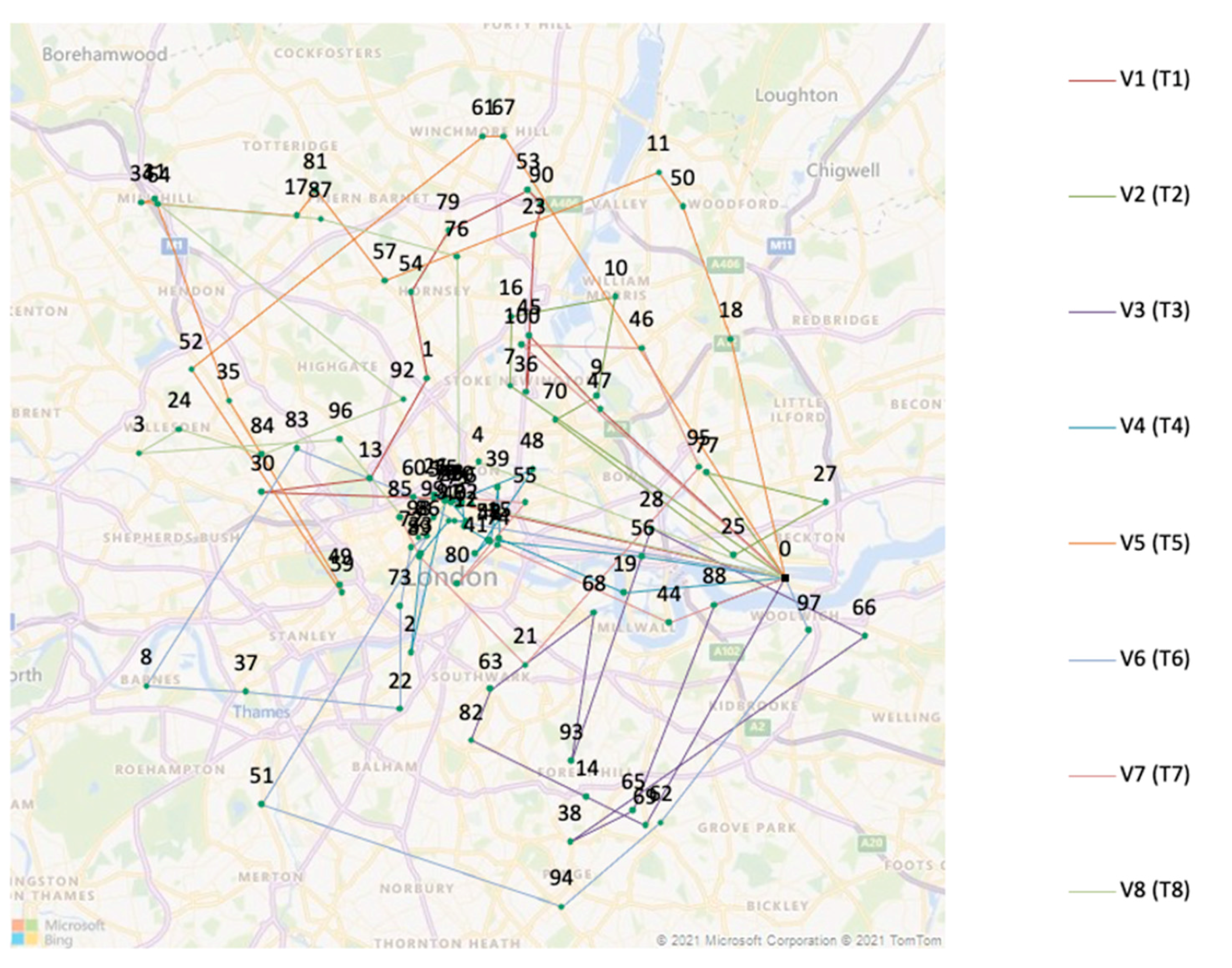
Appendix A shows 100 randomly generated passengers and their locations.

Table 2. The results for solving the problem with various numbers of EVs.

No. of EVs	No. of Maximum Served Customers	Delivery Cost 1	No. of Bags	Cost per Bag
3	43	GBP 152.1	90	1.69
4	59	GBP 200.4	120	1.67
5	72	GBP 249.0	150	1.66
6	88	GBP 297.2	178	1.67
7	98	GBP 343.2	208	1.65
8	109	GBP 387.7	235	1.65

¹ Delivery cost, including initial electric charge (GBP 37.24) and cost per mile without drivers’ salaries.

shows that 8 EVs are required to serve these 100 passengers. Using the spreadsheet solver tool for the first scenario (i.e., one hub/depot at the LCY), the total travel distance is 377.40 miles during one shift (8 h), the total cost is GBP 335.66 (see Appendix B), and the optimal routes of 8 vehicles are shown in Figure 9.

In the second scenario (i.e., multiple logistic hubs/depots in Greater London), the center of gravity approach is used to calculate the optimal location of the logistics hubs with the following assumptions [24]:

-

The passenger’s location and the number of baggage are known.

-

The costs are only determined by the distances between a logistic hub and the passenger’s location without considering city traffic.

-

The land-use fee, labor fee, and future profits are not considered.

Based on the assumptions, distance is the only factor that needs to be considered. Denote that ${\overline{X}}_j$ is x-coordinate of logistic hub j, ${\overline{Y}}_j$ is y-coordinate of logistic hub j, $n_j$ is the number of passengers that logistic hub j serves, $x_i$ is x-coordinate of passenger i, $y_i$ is y-coordinate of passenger i, and $l_i$ is the number of baggage w.r.t passenger i, then the location of logistic hub j is defined by:

$${\overline{X}}_j=\frac{{{\displaystyle \sum }}_{i=1}^{n_j}{x}_{i }{l}_i}{{{\displaystyle \sum }}_{i=1}^{n_j}{l}_i}$$

(1)

$${\overline{Y}}_j=\frac{{{\displaystyle \sum }}_{i=1}^{n_j}{y}_{i }{l}_i}{{{\displaystyle \sum }}_{i=1}^{n_j}{l}_i}$$

(2)

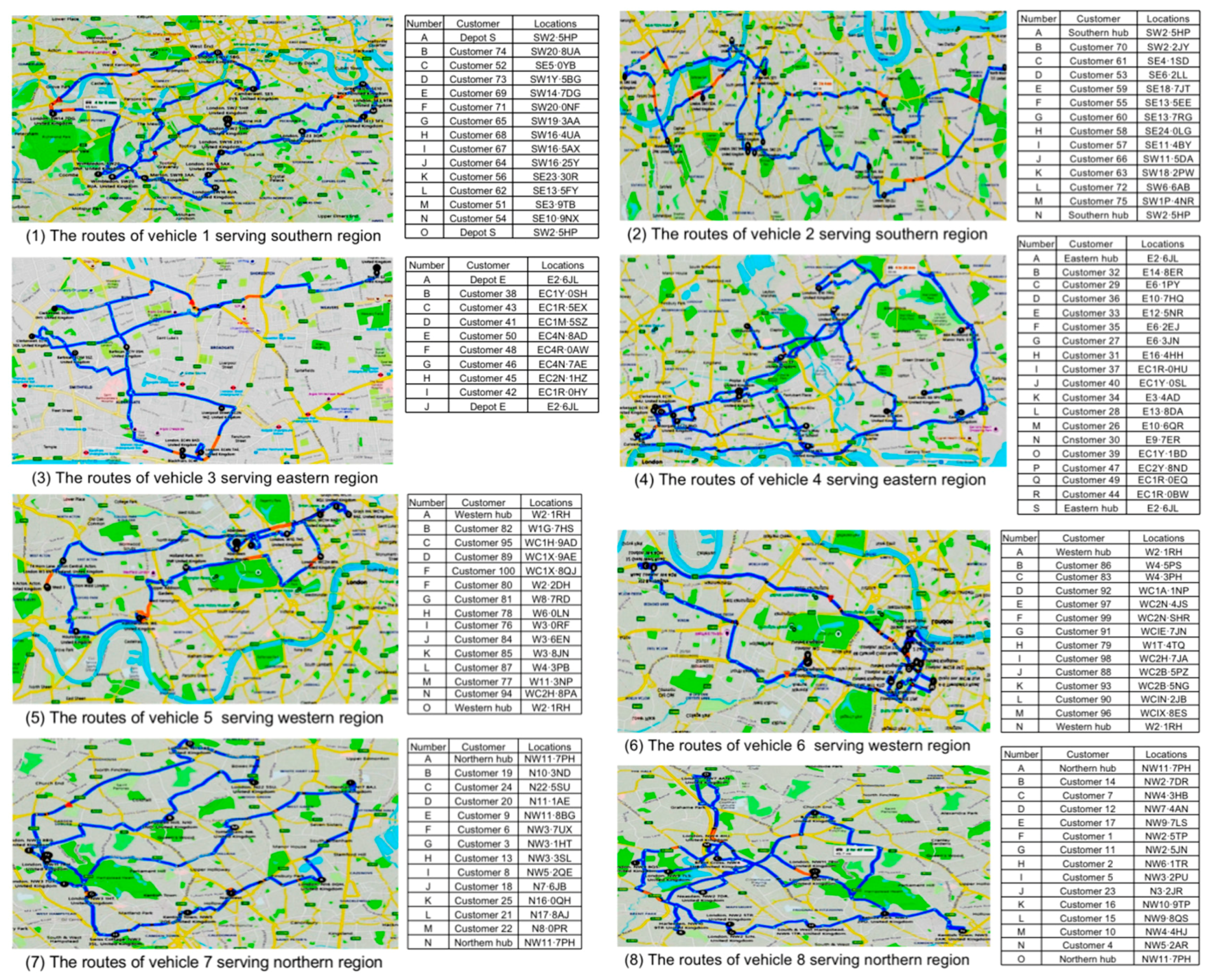
Greater London is divided into four regions with the corresponding postcodes such as North (NW and N), East (E and EC), South (SE and SW), and West (W and WC). In the baggage collection service, a certain logistic hub only serves one region. For example, EVs departing from the North hub serve passengers in postcodes NW and N. When applying the center of gravity approach, the locations of logistic hubs are shown in

Table 3. Locations of logistic hubs based on the center of gravity approach.

Region	Latitude	Longitude	Final Hub Locations
North (NW and N)	51.572	−0.185	Royal Mail
East (E and EC)	51.526	−0.047	Bethnal Green station
South (SE and SW)	51.454	−0.120	Brixton Hill post office
West (W and WC)	51.518	−0.172	Paddington station

.

However, it is difficult to set up the simulated coordinates as the final location of logistic hubs due to road traffic, passenger distribution, costs, and land availability. A logistic hub connecting to the highway, railway, and roadway can improve operation efficiency [25]. Land availability is an important factor. A new logistic hub requires unused lands and devices, which could be the main cost of building hubs [26]. For baggage delivery services, public hubs, including supermarkets, post offices, rail stations, and bus centers, are recommended as logistic hubs, which minimize the total cost compared to developing new hubs. In this case study, the final selected logistic hubs are the public places nearest to the simulated coordinates such as Royal Mail, Bethnal Green station, Brixton Hill post office, and Paddington station (see Table 3 and Figure 10). Using the spreadsheet solver tool for the second scenario, we achieve the following optimal solution. The total travel distance is 354.31 miles during one shift (8 h), the total cost is GBP 511.72 (see Appendix C), and the optimal routes of 8 vehicles are shown in Figure 11.

The comparison results of the solutions found in the first scenario and the second scenario are shown in

Table 4. Comparison of results for the first scenario (i.e., one hub at the LCY) and the second scenario (i.e., 4 logistic hubs in Greater London).

	Total Travel Distance (Mile)	Delivery Cost (GBP)	Number of Baggage	Cost per Baggage (GBP)
One hub at LCY	377.46	335.66	200	1.65
Four logistic hubs in Greater London	354.31	511.72	200	2.55

. The second scenario produces the solution with a shorter total travel distance. However, additional trucks could be required to deliver the baggage from the hubs to the LCY, increasing the fixed cost of each hub to purchase EVs, trucks, and land rental costs. Therefore, in the case study of the LCY, the first scenario is the best solution. It can balance total travel distance and cost. The first scenario’s collection operation is divided into various activities, including fixed costs and variable costs [27]. The variable costs (i.e., costs of each activity) are shown in

Table 5. Activity costs for the first scenario (i.e., one hub at the LCY).

Activities	Required Resources	Resource Cost	Cost for One Shift (8 h)
Transport service	Labor, electric charge	Labor: GBP 19,500 per annual	GBP 76.16
Collection service	Labor, AR label	Electric charge: GBP 0.1 per mile	GBP 335.66
		AR label: GBP 0.03	GBP 6

in which the labor cost is from the Totaljobs website, and the AR label is reusable. The equation of cost per baggage is computed as follows:

$$Activity costs per baggage=\frac{\mathrm{Labour} \mathrm{cost}+\mathrm{electric} \mathrm{charge}+\mathrm{AR} \mathrm{label} \mathrm{cost}}{\mathrm{Number} \mathrm{of} \mathrm{baggage} \mathrm{for} \mathrm{one} \mathrm{shift}}$$

(3)

4. Carbon Emission Reduction for the London City Airport

Three cases, defined by passenger’s preference for using the BFAT service, are analyzed to predict the popularity of baggage collection service and calculate the reduction of carbon emissions in the next few years [28,29]. The calculation steps for the reduction of carbon emissions are as follows:

-

Step 1: Using the simulation results to calculate the total distance that passengers traveled without baggage collection service.

-

Step 2: Using the CAA data and the proportion of private cars to calculate the total distance that passengers traveled by private cars.

-

Step 3: Using the average vehicle carbon emission data in the UK to calculate total carbon emission from private cars used by passengers.

-

Step 4: Using the proportion of passengers who switch from private cars to public transportation to calculate the potential carbon emission saving by baggage collection service.

-

Step 5: Using the predicted passenger number to calculate the carbon emission saving per passenger and carbon emission reduction per day.

The LCY served about 5 million passengers in 2019, 91.8% of which are from Greater London. Passenger demand is predicted up to 6 million by 2025 [20]. A total of 56% of the passengers use public transport to the LCY, while 44% of the passengers use private cars and taxis. Let $\Delta$ be the percentage of passengers who convert from private mode to public mode. In the case study, assume that 90% of passengers that are using private cars can switch to public transport, then $\Delta =44\times 90\%=39.6\%$, and the total travel distance to the LCY of 100 customers is 749.70 km. The equation of average carbon emissions is shown as follow:

$$\begin{array}{l}Average {CO}_2 emission per customer\\ =\frac{Total travel distance\times {CO}_2 per km\times percentage of customers used private cars and taxi}{Number of customers used private cars and taxi}\end{array}$$

(4)

where CO₂ per km is based on the ‘ASM Auto Recycling’ [30], i.e., the average CO₂ emission per vehicle is 125.1 kg/km in 2018, the CO₂ emission of private cars and taxis is 1.27 kg/km.

Total reduced CO₂ emission is defined by:

$$Total {CO}_2 reduction=Number of customers\times average {CO}_2 emission per customer\times \Delta$$

(5)

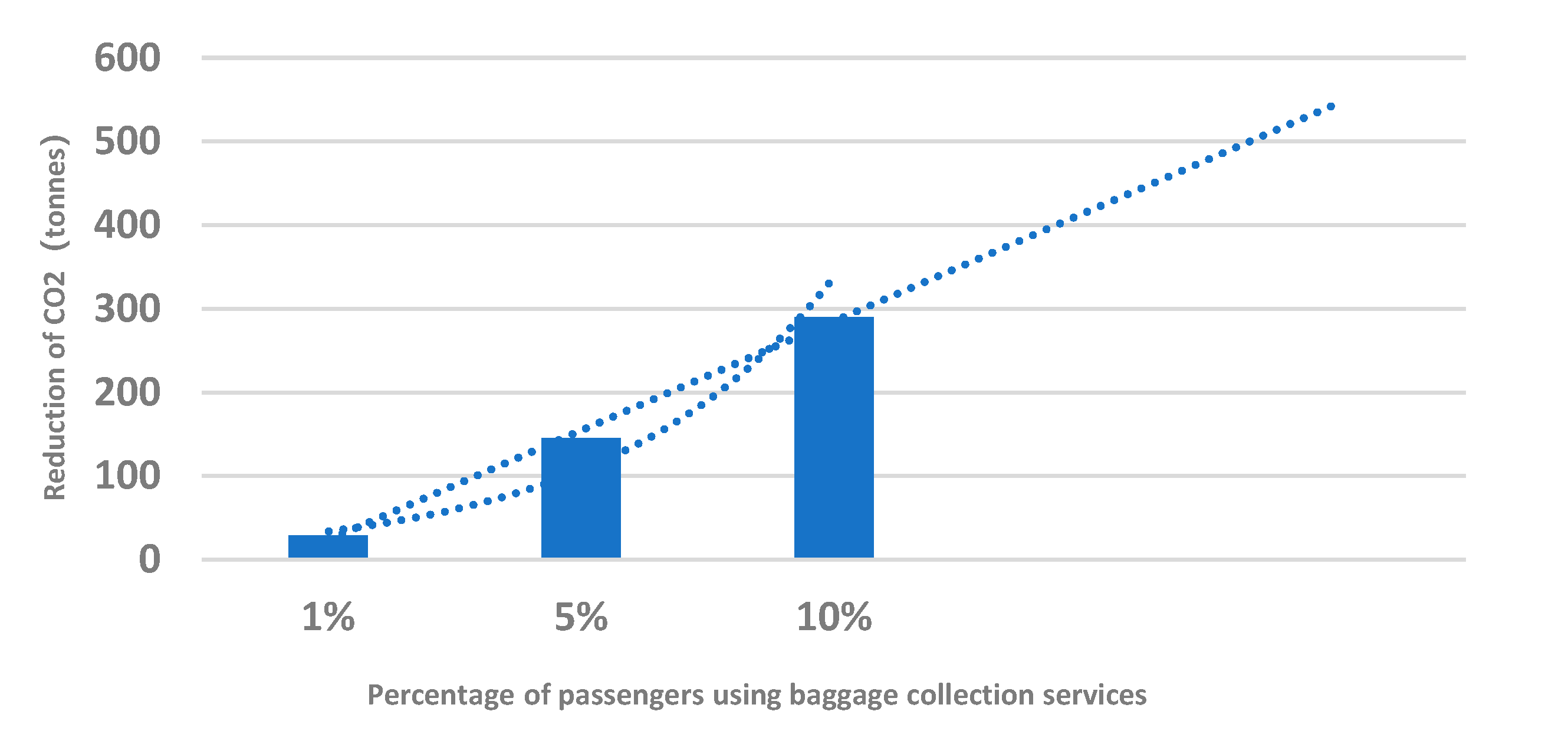
In the first case (i.e., low preference for the BFAT service), we assume that 1% of passengers will use the baggage collection service by 2025. The results show that the total daily reduced CO₂ emission for 160 customers is 79.48 kg. As a result, the baggage collection service will reduce 29.01 tonnes of carbon emissions annually. In the second case (i.e., medium preference for the BFAT service), we assume that 5% of passengers will use the baggage collection service by 2025. The total daily reduced CO₂ emission for 360 customers is 397.40 kg (i.e., 145.05 tonnes of carbon emissions annually). In the third case (i.e., high preference for the BFAT service), we assume that 10% of passengers will use the baggage collection service by 2025. The total daily reduced CO₂ emission for 360 customers is 794.79 kg (i.e., 290.10 tonnes of carbon emissions annually). Figure 12 shows the comparison results of CO₂ emission reduction in three cases.

5. Application of AR for Baggage Tracking

Late deliveries, damaged baggage, and mishandled baggage can all be red flags in baggage collection service, therefore, baggage tracking is proposed as a solution. With the rapid development of technologies such as radio frequency identification (RFID), barcodes, QR codes, and AR, courier and delivery companies have been tracking parcels and providing customers with real-time information for quite some time. Currently, many delivery companies use simple barcodes for baggage handling, which is cheap and simple technology. However, barcodes require a handheld scanner with 60–70% read rates, which reduces staff efficiency and increases the frequency of mishandling baggage. Many delivery companies use RFID for baggage identification and tracking, which is expensive and requires an additional reading scanner [31]. AR technology with QR codes allows passengers to track baggage in real-time without handheld devices. The technology can decrease the need for manual processing and free up staff for other value-adding tasks. Passengers can even check their baggage by themselves with a simple mobile app. The procedure is described as follows (see Figure 13):

-

Step 1: Collect passenger’s baggage.

-

Step 2: Assign a QR code to each baggage.

-

Step 3: Deliver the baggage to the hub.

-

Step 4: Deliver the baggage onto the aircraft.

-

Step 5: Scan the QR code for a double check when custody changes between carriers.

-

Step 6: Deliver the baggage to the passenger’s destination.

-

Step 7: Passengers or staff scan the QR code to check baggage-passenger information to avoid mishandling.

AR technology with QR codes is an easy and cost-effective way to obtain baggage tracking records. It reduces the number of lost, delayed, and mishandled baggage and improves the customer experience. With AR glasses or AR-based mobile app, the baggage collection service will reduce the cost and time of baggage double-checking, as well as help eliminate baggage fraud. The goals of QR codes and AR-based baggage collection service implementation are to increase customer satisfaction, eliminate mishandling, improve information visibility, reduce manual labor costs, and reduce delivery delays [32]. Hence, the AR technology for baggage tracking system is proposed to integrate into the BFAT for the efficient management of the baggage collection and transport network.

6. Conclusions and Future Work

The transformation of the passenger baggage experience is gathering pace. A transparent, real-time tracking baggage collection service will make a more relaxing journey that will encourage passengers to use more public transport (after the burden of baggage is removed) for air quality improvement. This paper investigates a baggage collection service network design problem using vehicle routing strategies and AR technology toward the goal. A spreadsheet solver tool, integrating MCWS and DBCA, is adopted to solve the problem and simulate the optimal routing networks and logistic hubs. This tool can solve to optimality the problem with a maximum of 200 nodes. The LCY is used as a case study to demonstrate the efficiency of the proposed model and tool for reducing airport-related carbon emissions. The results show that the model is efficient for the actual airport service. It can reduce 290.10 tonnes of carbon emissions annually in the case that 10% of passengers will use the baggage collection service by 2025.

In the baggage collection network, AR technology with QR codes makes the service quicker and easier to track baggage-passenger information. It provides extra information about the baggage journey and enables a faster process for baggage double-checking by passengers or staff to reduce baggage mishandling.

This paper aims to demonstrate the efficiency of the proof-of-concept planning model toward BFATs. The adopted spreadsheet solver tool has also achieved very good performance for the GVRP in the baggage collection network design. For larger-sized instances, other well-known metaheuristic algorithms (e.g., genetic algorithm, tabu search, simulated annealing, etc.) could be developed to improve the solution performance.

In addition, the model can be applied for other airports such as London Heathrow Airport, Manchester Airport, etc. A comparison of implementing the model for the airports will then be made to evaluate its applicability. Another future research approach is the baggage collection network design under the risk of unexpected failures to mitigate the impact of disruptions on the performance of network design.

References

1. IATA. Airline Industry Financial Forecast, Outlook for the Global Airline Industry (April Update). Available online: https://www.iata.org/en/iata-repository/publications/economic-reports/airline-industry-economic-performance---april-2021---report/ (accessed on 27 April 2021).
2. Urban Turbine Homepage. Available online: https://urbanturbine.org (accessed on 20 May 2021).
3. Mara, S.T.W.; Kuo, R.J.; Asih, A.M.S. Location-routing problem: A classification of recent research. Int. Trans. Oper. Res. 2021, 28, 1–43. [Google Scholar] [CrossRef]
4. Kallehauge, B.; Larsen, J.; Madsen, O.B.; Solomon, M.M. Vehicle routing problem with time windows. In Column Generation; Springer: Boston, MA, USA, 2005; pp. 67–98. [Google Scholar]
5. Karakatič, S.; Podgorelec, V. A survey of genetic algorithms for solving multi depot vehicle routing problem. Appl. Soft Comput. 2015, 27, 519–532. [Google Scholar] [CrossRef]
6. Brandão, J.C.S.; Mercer, A. The multi-trip vehicle routing problem. J. Oper. Res. Soc. 1998, 49, 799–805. [Google Scholar] [CrossRef]
7. Baldacci, R.; Battarra, M.; Vigo, D. Routing a heterogeneous fleet of vehicles. In The Vehicle Routing Problem: Latest Advances and New Challenges; Springer: Boston, MA, USA, 2008; pp. 3–27. [Google Scholar]
8. Erdoğan, S.; Miller-Hooks, E. A Green Vehicle Routing Problem. Transp. Res. Part E Logist. Transp. Rev. 2012, 48, 100–114. [Google Scholar] [CrossRef]
9. Bektaş, T.; Laporte, G. The pollution-routing problem. Transp. Res. Part B Methodol. 2011, 45, 1232–1250. [Google Scholar] [CrossRef]
10. Franceschetti, A.; Honhon, D.; Van Woensel, T.; Bektas, T.; Laporte, G. The time-dependent pollution-routing problem. Transp. Res. Part B Methodol. 2013, 56, 265–293. [Google Scholar] [CrossRef] [Green Version]
11. Koç, Ç.; Bektaş, T.; Jabali, O.; Laporte, G. The fleet size and mix pollution-routing problem. Transp. Res. Part B Methodol. 2014, 70, 239–254. [Google Scholar] [CrossRef]
12. Zhang, W.; Gajpal, Y.; Appadoo, S.S.; Wei, Q. Multi-Depot Green Vehicle Routing Problem to Minimize Carbon Emissions. Sustainability 2020, 12, 3500. [Google Scholar] [CrossRef] [Green Version]
13. Ge, X.; Ge, X.; Wang, W. A path-based selection solution approach for the low carbon vehicle routing problem with a time-window constraint. Appl. Sci. 2020, 10, 1489. [Google Scholar] [CrossRef] [Green Version]
14. Ghorbani, E.; Alinaghian, M.; Gharehpetian, G.B.; Mohammadi, S.; Perboli, G. A Survey on Environmentally Friendly Vehicle Routing Problem and a Proposal of Its Classification. Sustainability 2020, 12, 9079. [Google Scholar] [CrossRef]
15. Felipe, Á.; Ortuño, M.T.; Righini, G.; Tirado, G. A heuristic approach for the green vehicle routing problem with multiple technologies and partial recharges. Transp. Res. Part E Logist. Transp. Rev. 2014, 71, 111–128. [Google Scholar] [CrossRef]
16. Schneider, M.; Stenger, A.; Goeke, D. The Electric Vehicle-Routing Problem with Time Windows and Recharging Stations. Transp. Sci. 2014, 48, 500–520. [Google Scholar] [CrossRef] [Green Version]
17. Omidvar, A.; Tavakkoli-Moghaddam, R. Sustainable vehicle routing: Strategies for congestion management and refueling scheduling. In Proceedings of the IEEE International Energy Conference (ENERGYCON ’12), Florence, Italy, 9–12 September 2012; pp. 1089–1094. [Google Scholar]
18. International Energy Agency. Global EV Outlook 2018. Available online: https://www.iea.org/reports/global-ev-outlook-2018 (accessed on 20 March 2021).
19. You Could Travel. Guide to Suitcase and Luggage Sizes. Available online: https://www.youcouldtravel.com/travel-blog/understanding-suitcase-sizes (accessed on 30 March 2021).
20. Civil Aviation Authority. Passenger Survey Report. Available online: https://www.caa.co.uk/Data-and-analysis/UK-aviation-market/Consumer-research/Departing-passenger-survey/2019-Passenger-survey-report/ (accessed on 25 March 2021).
21. Alumur, S.A.; Kara, B.Y. Network hub location problems: The state of the art. Eur. J. Oper. Res. 2008, 190, 1–21. [Google Scholar] [CrossRef] [Green Version]
22. Arrival. The Arrival Van. Changing the Way Your City Moves. Available online: https://arrival.com/?id=2 (accessed on 23 April 2021).
23. Department for Transport. European Union (EU) Rules on Drivers’ Hours and Working Time: Simplified Guidance (2015). Available online: https://assets.publishing.service.gov.uk/government/uploads/system/uploads/attachment_data/file/856360/simplified-guidance-eu-drivers-hours-working-time-rules.pdf (accessed on 23 March 2021).
24. Hansen, W.G. Accessibility and Residential Growth. Ph.D. Thesis, Massachusetts Institute of Technology, Cambridge, MA, USA, 1959. [Google Scholar]
25. Zhao, X. Based on gravity method of logistics distribution center location strategy research. In Proceedings of the International Conference on Logistics Engineering, Management and Computer Science (LEMCS 2014), Shenyang, China, 24–26 May 2014; Atlantis Press: Paris, France, 2014; pp. 586–589. [Google Scholar]
26. Alam, S.A. Evaluation of the potential locations for logistics hubs: A case study for a logistics company. Master’s Thesis, KTH Royal Institute of Technology, Stockholm, Sweden, 2013. [Google Scholar]
27. Duncan, I. Controlling Expenses: The Key to Profitability in a Recession. CMA-The Management Accounting Magazine (1992). Available online: https://www.referenceforbusiness.com/small/Eq-Inc/Fixed-and-Variable-Expenses.html#ixzz6sNYYXzaF (accessed on 25 March 2021).
28. Kishita, Y.; Ohishi, Y.; Uwasu, M.; Kuroda, M.; Takeda, H.; Hara, K. Evaluating the life cycle CO2 emissions and costs of thermoelectric generators for passenger automobiles: A scenario analysis. J. Clean. Prod. 2016, 126, 607–619. [Google Scholar] [CrossRef]
29. Börjeson, L.; Höjer, M.; Dreborg, K.H.; Ekvall, T.; Finnveden, G. Scenario types and techniques: Towards a user’s guide. Futures 2006, 38, 723–739. [Google Scholar] [CrossRef]
30. ASM Auto Recycling. Car CO2 Emissions. Available online: https://www.asm-autos.co.uk/blog/car-co2-emissions/ (accessed on 25 April 2021).
31. IATA. Radio Frequency Identification (RFID). Available online: https://www.iata.org/en/programs/ops-infra/baggage/rfid/ (accessed on 27 April 2021).
32. IATA. IATA Resolution 753: Baggage Tracking. Available online: https://www.iata.org/whatwedo/stb/Documents/baggage-tracking-res753.pdf (accessed on 25 April 2021).
Figure 1. A flowchart of the integrated algorithm for GVRP.
Sustainability 14 00212 g001
Figure 2. The structure of the spreadsheet solver tool.
Sustainability 14 00212 g002
Figure 3. Console spreadsheet.
Sustainability 14 00212 g003
Figure 4. Locations spreadsheet.
Sustainability 14 00212 g004
Figure 5. Distances spreadsheet.
Sustainability 14 00212 g005
Figure 6. Vehicles spreadsheet.
Sustainability 14 00212 g006
Figure 7. Solution spreadsheet.
Sustainability 14 00212 g007
Figure 8. Visualization spreadsheet.
Sustainability 14 00212 g008
Figure 9. The optimal route map of 8 vehicles for the first scenario (i.e., one depot).
Sustainability 14 00212 g009
Figure 10. London postcode districts and the locations of logistic hubs.
Sustainability 14 00212 g010
Figure 11. The optimal route map of 8 vehicles for the second scenario (i.e., 4 hubs/depots).
Sustainability 14 00212 g011
Figure 12. Carbon emission reduction in three cases.
Sustainability 14 00212 g012
Figure 13. The procedure of applying AR for baggage tracking in the BFAT service.
Sustainability 14 00212 g013