Abstract
LCAs of electric cars and electrolytic hydrogen production are governed by the consumption of electricity. Therefore, LCA benchmarking is prone to choices on electricity data. There are four issues: (1) leading Life Cycle Impact (LCI) databases suffer from inconvenient uncertainties and inaccuracies, (2) electricity mix in countries is rapidly changing, year after year, (3) the electricity mix is strongly fluctuating on an hourly and daily basis, which requires time-based allocation approaches, and (4) how to deal with nuclear power in benchmarking. This analysis shows that: (a) the differences of the GHG emissions of the country production mix in leading databases are rather high (30%), (b) in LCA, a distinction must be made between bundled and unbundled registered electricity certificates (RECs) and guarantees of origin (GOs); the residual mix should not be applied in LCA because of its huge inaccuracy, (c) time-based allocation rules for renewables are required to cope with periods of overproduction, (d) benchmarking of electricity is highly affected by the choice of midpoints and/or endpoint systems, and (e) there is an urgent need for a new LCI database, based on measured emission data, continuously kept up-to-date, transparent, and open access.
1. Introduction
Both battery electric vehicles (BEVs) and electrolytic hydrogen play a key role in the context of the ongoing energy transition, which is required to keep global warming “well below two degrees Celsius above pre-industrial levels” as agreed in 2015 at the Conference of the Parties (COP21) meeting in Paris. BEVs are considered as an important contributor to reduce the carbon intensity of the transportation sector. This sector represents 25% of the EU’s total greenhouse gases (GHG) emissions [1]. Fuel Cell Electric Vehicles (FCEVs) powered with clean hydrogen, including electrolytic hydrogen, are expected to complement BEVs. FCEVs are best suited for applications with long-range requirements, heavier payloads, and a high need for flexibility. The role of clean hydrogen goes well beyond the decarbonization of the transport sector. Thus, in the recent European Green Deal [2] hydrogen has been identified as a key instrument for meeting the net-zero global warming emissions by 2050. According to the vision by the Hydrogen Council [3], by 2050 hydrogen demand could increase 10-fold and account for almost one fifth of the total final energy consumed. Beyond decarbonizing the transportation sector, hydrogen is expected to act as a clean feedstock and energy carrier for industry, to decarbonize the heat and power sectors, and to allow integration, storage, and transportation of an increasing share of renewable electricity.
In LCAs for BEVs and hydrogen produced by electrolysis, electricity has a dominant contribution [1,4,5,6], not only in the use-phase, but also in the production of the materials. The percentage of CO2 emissions from electricity for metals production (Ecoinvent V3.5, “cut-off” database) is in the range of 30–56% (e.g., Aluminum 56%, Copper 35%, Gold 36%, Lead 30%, Nickel 31%, Silver 52%, Zinc 50%). For woven textile (Polyester, 70 dTex) the percentage is higher (70–80%). For BEVs, electrolytic hydrogen, and other products like household appliances such as washing machines, vacuum cleaners, and flat irons, the choice of data for electricity is therefore highly relevant. Common practice in LCA for household appliances is that the European average consumption mix is applied (reasoning: these appliances are used all over Europe), except for specific cases (ex-post LCA) where predominantly the country consumption mix data are taken. An analysis of 38 papers on LCAs of washing machines (search in Scopus on ‘LCA washing machine’) revealed that in more than 80% of the papers the origin of the electricity was not specified, which suggests that the author was not aware of the big differences in data on electricity.
With regard to the electricity that is purchased, two distinct approaches are explained and defined in the GHG Protocol Scope 2 Guidance [7]: ‘location-based’ and ‘market-based’. Location-based is the situation where the calculation uses the average regional electricity mix from the grid. Market-based is the situation where the calculation is based on electricity that is purchased from a selected (renewable energy) supplier who guarantees the origin. It is obvious that location- and market-based approaches can deliver very different LCA results.
Modern LCI databases have two distinct datasets for electricity: ‘electricity by country’ and ‘electricity by fuel’ (with country adaptations). The ‘electricity by country’ is either the ‘production mix’ (i.e., the average emissions of the electricity production) or the ‘consumption mix’ (i.e., the average emissions of the electricity mix of the grid, including net imports). LCI country data from the current LCI databases are ex-post and location-based. They are suitable for retrospective LCA studies dealing with an existing generic product or technology. Other LCA-based calculations, such as Environmental Product Declarations, use ex-post LCAs in combination with the market-based approach. This is because the aim is to describe the actual emissions of a product as accurately as possible. Product and process innovation in R&D require ex-ante LCAs [8], since they deal with alternative (future) situations. These LCA studies should apply an ex-ante assumption on a specific future mix of solar, wind, hydro, and fossil power (rather than the ex-post country mix).
In general, LCA practitioners are aware of the high uncertainties in LCA. However, there is a general feeling among LCA practitioners that data on electricity are rather accurate in LCI databases. Therefore, they take the electricity data for granted. Only specialists know that there are issues with data quality [9]. Even though there is an LCA harmonization initiative for hydrogen [6,10], Product Environmental Footprint Category Rules (PEFCRs) for the European market are not yet available for electricity nor for hydrogen. This paper does not go into these details but shows that there are inconvenient differences between well-established LCI databases.
To explain the issues of this paper in a practical way, the Well-to-Wheel LCA benchmarking study [11] is taken as an example. Figure 1 shows that the advantage of a battery electric vehicle, compared to a gasoline or diesel internal combustion engine (ICE) vehicle, is only evident when the carbon footprint of the electricity for driving is low enough.
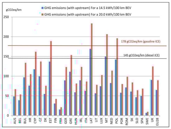
Figure 1.
GHG emissions due to the use of electric vehicles in the European Union, calculated by using C-intensity data for electricity from IEA for the year 2013. Source: [11] 1361-9209/© 2017 The Authors. Published by Elsevier Ltd. This is an open access article under the CC BY license (http://creativecommons.org/licenses/BY/4.0/ (accessed on 20 April 2020)).
Note that the emission data of Figure 1 are not taken directly from LCA databases, but from International Energy Agency (IEA) consumption mix databases, with corrections for power losses in the grid to the consumer (from Ecoinvent), and inclusion of the upstream GHG emissions from the electricity supply chain. The boundaries of the assessment in Figure 1 do not include the car battery, which is estimated at a range of 36 gCO2/km to 40 gCO2/km [12,13] for a 35.8 kWh battery capacity. The diesel and gasoline lines are from [14].
The underlying question in Figure 1, however, is the accuracy of the electricity consumption mix data in the several countries: (1) are they measured or calculated by parameterization? (2) are they up-to-date enough? or (3) would it be better to have here the predicted data for 2025 or 2030? The relevance of up-to-date or future data is given by the fact that most of the LCA R&D studies are ex-ante oriented (what can be improved in the future?) rather than ex-post (what was the past situation?).
Another issue is the temporal use of electricity. In the case of BEV, the batteries may be loaded in periods of overcapacity of windmills or Photovoltaic (PV) cells.
Given all uncertainties and inaccuracies on a country level, is it better to apply the EU-27 consumption mix for the base case (instead of a country consumption mix), and apply additional cases for specific renewable sources (e.g., wind, solar)?
Last but not least, there is the issue of nuclear power. There is no doubt that it mitigates climate change, but what about the nuclear risks? Is there a need for weighting climate risks and nuclear risks in LCA benchmarking studies?
Given all these kinds of questions, uncertainties, and inaccuracies, the research questions of this paper on electricity are:
- What is the uncertainty in applying LCI data from existing leading databases?
- What is the effect of the fact that the LCI data are, in practice, 4–8 years old on average?
- How to deal with the fluctuations over time of the carbon intensity of electricity and time-related allocation on a time scale of 1 h?
- When does it make sense to apply a Guarantee of Origin or the residual mix, and when is it better to apply the country consumption mix?
- How to deal with nuclear power in relation to greenhouse gas emissions (the issue of comparing ‘apples with oranges’ by the selection of midpoints and endpoints in LCA)?
In the following text of this paper, the next section deals with specifications and regulations which are related to electricity in LCA. Then, the five research questions are dealt with in the subsequent sections. The paper is concluded with two sections on the Discussion and Conclusions.
2. Methods: Specifications and Regulations
Right from the beginning years of LCA the choice of LCI data for electricity was an important issue. The first approach was to select the nearest (set of) power plants, following the logic that big cities and big industrial harbor regions had their own power plants. This ‘production mix’ was either on a regional level or on a country level [15]. Then there was an awareness that, especially in Europe, small countries import electricity, so that for these countries the ‘consumption mix’ is more relevant than the ‘production mix’. The first ‘country consumption mix’ comprehensive dataset was developed in 2007 for Ecoinvent Version 2 [16].
Maps on the country consumption mix carbon intensities, see Figure 2, are important to make the world population aware of the responsibilities of their governments with regard to climate change mitigation.
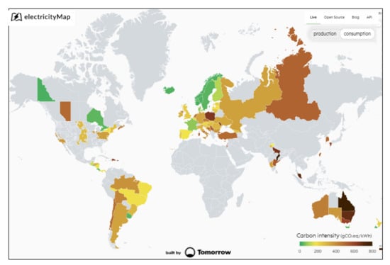
Figure 2.
Carbon intensity of electricity per country (‘consumption mix’) from the hourly real-time electricity map accessed on 29 April 2021 at 10 a.m. CET [17].
Figure 2 shows the enormous differences of carbon intensity among countries. However, the question is how to deal with it in LCA. By far, most of the LCA work is focused on improvements on product level (ex-ante ‘attributional LCA’), often on a global scale or the scale of the EU, so the current, most common, ‘country consumption mix’ approach might not always be the best choice in LCA.
Due to its general nature, the LCA standard ISO 14044:2006 does not specify which data on electricity should be selected in which case, other than with the statement that “data selected for an LCA depend on the goal and the scope of the study“ (§4.2.3.5), and with regard to data quality
” …should address the following: (a) time-related coverage: the age of data …; (b) geographical coverage: geographical area from which data for unit processes should be collected to satisfy the goal of the study;…” (§4.2.3.6.2).
This simply underlines that the selection of electricity data, as the other background data, is governed by the specific goal of the LCA study.
The International Reference Life Cycle Data system manual (ILCD) [18] reinforces the importance of selecting data based on the LCA goal, and provides a specific example for electricity in Section 6.8.3 [18]:
“LCI data should represent the smallest, appropriate geographical unit, depending on the goal of the LCI/LCA study and the intended applications. If e.g., the use of an energy-using consumer product in France would be the scope of the data set, the corresponding electricity market consumption mix …. were to be considered, i.e., not European or Global average conditions”.
Similarly, for an LCA on product manufacturing, the smallest, appropriate, geographical unit is often the ‘production mix’ on regional level (when import data are not known). There are many situations where the local production mix of two or three power plants near a manufacturing plant give a plausible better result than the country consumption mix, since it is a better fit with the physical reality.
Publicly Available Specification (PAS 2050) [19] rules are along the same lines as the rule of the ILCD: PAS 2050 advises also the country average in Section 7.9.3b [19]:
“… for electricity and heat delivered via a larger energy transmission system, secondary data that is as specific to the product system as possible (e.g., average electricity supply emission factor for the country in which the electricity is used)”.
Note that this suggests the ‘country consumption mix’. Only when the electricity is delivered by a stand-alone source, the data of that specific source type must be applied. Both ILCD and PAS follow more or less the reasoning of the physical relationship (the flow of the electrons). However, PAS accepts the use of GOs in Section 7.9.4:
“Note 3. In countries where the flow of renewable electricity is accurately accounted for, the requirement 7.9.4.2 allows companies using renewable electricity, or purchasing renewable electricity through a dedicated tariff, to use the GHG emission of the renewable electricity (rather than grid-average carbon intensity) when calculating the emissions arising from their processes”.
The applicability of GOs in LCA is further discussed in Section 3.4 below.
In contrast to GOs, offsetting (by “credits”) is not allowed in PAS 2050. Section 5.8 [19]:
“GHG emissions offset mechanisms, including but not limited to voluntary offset schemes or nationally or internationally recognized offset mechanisms, shall not be used at any point in the assessment of the GHG emissions of the product. Note… The use of an energy source that results in lower GHG emissions to the atmosphere and therefore achieves a lower emission factor, such as renewable electricity (see 7.9.4) or …, is not a form of offsetting”.
The GHG protocol [20] recommends GO or residual mix where available:
“As with data from other emission sources, companies should select electricity emission factors that are geographically specific to the electricity sources used in the product inventory. When an electricity supplier can deliver a supplier-specific emission factor and these emissions are excluded from the regional emission factor, the supplier’s electricity data should be used. Otherwise, companies should use a regional average emission factor for electricity to avoid double counting”.
However, in the GHG Protocol Scope 2 Guidance [7], section “new reporting requirements”, a dual reporting is foreseen:
“Companies with any operations in markets providing product or supplier-specific data in the form of contractual instruments shall report scope 2 emissions in two ways and label each result according to the method: one based on the location-based method, and one based on the market-based method. This is also termed ‘dual reporting’”.
In the Product Environmental Footprint (PEF) project of the EU [21] there is a distinction between the production phase and the use phase. For the production phase, a hierarchical approach for selecting the electricity mix has been developed (Section 7.13.1 [21]). This is basically a further specification of the philosophy of the GHG protocol and favors the market approach rather than the physical/location approach. The first option is to take electricity data from the purchase contract (and ask suppliers for more detailed information). As a second option, supplier-specific total electricity mix shall be selected. In fact, as the supplier often only specifies electricity mixes per type of source (e.g., biomass, wind, hydropower), PEF (GaBi) provides data on ‘electricity per fuel’ per country. When no details are known, as the last option the country, ‘residual’ mix must be applied. Residual means that the Guarantee of Origin contracts are subtracted from the total consumption data, to avoid administrative double counting of GOs.
Offsets are not allowed in PEF [22] (Section 4.4.11):
“Offsets shall not be included in the impact assessment of a PEF study, but may be reported separately as additional environmental information”.
For the use phase PEF prescribes the use of consumption grid mix (Section 7.13.6 [21]). PEF is in line with ISO 14067:2018 (on the Carbon Footprint of products) that allows GOs in §6.4.9.4, and prohibits carbon offsetting in §3.1.1.7 + Note 1.
The Renewable Energy Directive II of the EU (which is “on the promotion of the use of energy from renewable sources”) [23] is most specific on the way the carbon intensity is to be calculated in the transport sector (Article 27-3-b paragraph 3):
“Where electricity is used for the production of renewable liquid and gaseous fuels of non-biological origin the average share of electricity from renewable sources in the country of production, as measured two years before the year in question, shall be used to determine the share of renewable energy. However, electricity obtained from direct (i.e., physical) connection to an installation generating renewable electricity may be fully counted as renewable electricity provided that the installation (a) comes into operation after or at the same time as the installation producing… and (b) is not connected to the grid or is connected to the grid but no electricity taken from it…”
Electricity that has been taken from the grid may be counted as fully renewable provided that it is produced exclusively from renewable sources and the renewable properties and other appropriate criteria have been demonstrated, ensuring that the renewable properties of that electricity are claimed only once [24]. The details on the implementation of the use of renewable electricity which is purchased from the grid are still to be developed. It will likely be based on existing GO and additional requirement to fulfil Recital 90:
“The Commission should develop, by means of delegated acts, a reliable Union methodology to be applied where such electricity (of renewable origin) is taken from the grid. That methodology should ensure that there is a temporal and geographical correlation between the electricity production unit with which the producer has a bilateral renewables power purchase agreement … Furthermore, there should be an element of additionally, meaning that the fuel producer is adding to the renewable deployment or to the financing of renewable energy”.
In other words: additional elements are required to make the GO acceptable, such as financing the renewable power plant or other elements in the contract that make sure that the contract adds directly to the development of renewable energy.
Note that the relevance of the use of GOs in LCA depends on the goal of the study. Further deliberation on the subject of GOs and its counterpart, the Residual mix, is given in Section 3.4 below.
3. Results of the Analyses
3.1. Inaccuracy of LCI Data in Existing Leading Databases
The LCI data on specific technologies of electricity production show a wide variability in existing literature [25], so the quest for accuracy is not easy even given the fact that the only impact considered in this study is C-footprint. For fossil fuels the most important aspects are the energy recovery efficiency and the flue gas cleaning systems. For wind and solar power, the most important aspects are efficiency and the electricity mix used for the production, installation and maintenance of the infrastructure [25].
The three leading LCI databases—Ecoinvent, European reference Life Cycle Database (ELCD), and PEF (GaBi)—solve this issue basically by parametrization of the problem in a top-down approach. The basis is the country market mix of energy types (coal, gas, oil, wind, solar, bio, geothermal, nuclear, etcetera) from IEA or European Network of Transmission System Operators for Electricity (ENTSO-E) databases [16]. For each energy source, an LCI study is selected as a base case and, in some cases, parameterized to cope with the differences in specific countries. This top-down approach has the advantage that LCIs for the different countries can be generated in a rather easy and flexible way by adjusting the parameters of the model. The disadvantage, however, is the inaccuracy of the results (geographical and technological specificity is not fully accounted for) and the lack of transparency (the algorithms of the parameterization are not published). As a consequence, it is not possible to make a comparative assertion on which database is better than the other.
The carbon intensity of the electricity consumption can also be determined country by country as done in [11]. Country specific data from various IEA sources were first combined to get the electricity supplied to a national network including the trade. Power losses for transport were based on Ecoinvent calculations. CO2 emissions from fuel combustion were calculated using fuel specific emission factors from the intergovernmental panel on climate change (IPCC) 2006. Upstream emissions of the fossil fuel supply chains (normally 10–20% of the combustion emissions [11,25]) were calculated separately and added. Missing in this approach are the carbon emissions from the construction of the facilities. These emissions are negligible in countries with a low share of renewables but will become less and less negligible as this share increases. In Table 1, the carbon intensity results from such calculations for medium voltage electricity are shown (column a) and compared with data from LCI leading databases.

Table 1.
The carbon intensity of the consumption mix at medium voltage (MV) and the residual mix of electricity for some European countries. Note: the reference of PEF (Gabi) is: Thinkstep AG (2019–2024): LCI datasets for EU Environmental Footprinting (EF) implementation 2019–2024, EF Database 2.0, in Simapro, http://lcdn.thinkstep.com (accessed on 5 May 2021).
It can be concluded from Table 1 that the uncertainty in the carbon intensity data in the LCA databases is up to 35% (with the exception of FR, because of the high share of nuclear power and the higher inaccuracy of its CO2 emissions compared to fossil fuels). The calculations have been made in November 2019, using SimaPro software. The same IPCC 2013 GWP 100 year dataset has been applied for all columns. The uncertainty of data on other pollutants (e.g., SO2eq, NO2eq) is even higher, as documented in [25]. These gate-to-gate emissions of the individual power plants, however, are available in the European Pollutant Release and Transfer Register (E-PRTR) database [26].
Table 1 also shows data on the Residual mix in column h. The importance of residual mix is discussed in Section 3.4.
3.2. Outdated Data in a Rapid Changing World
Given the awareness of the climate change and the Paris agreement, EU countries are rapidly changing their production mix of electricity. As a result, the LCI data in existing databases are outdated in nearly all cases (accessed November 2019):
- The reference year in ELCD V3.2 is 2008;
- The reference year in Ecoinvent V3.5 is 2014;
- The reference year in PEF (GaBi) is 2013.
Data on the carbon intensity from the EU in the past are shown in Figure 3, available at the database of the European Environment Agency (EEA) [27].
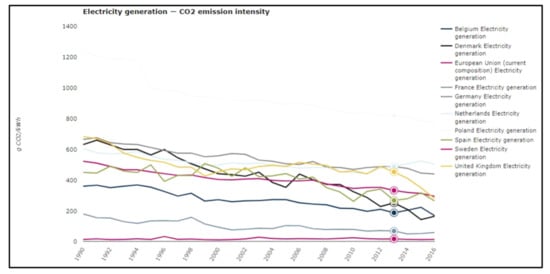
Figure 3.
Carbon intensities (power plants gate-to-gate) within the EU for the period 1990–2016 [27].
Figure 3 shows a steady decline of the carbon intensity in the EU. The decline is different for each country, and varies from year to year. For the last period of 3 years, 2013–2016, the decline in the EU was from 333 to 296 g CO2/kWh (11%), in UK from 454 to 281 g CO2/kWh (38%), and in DK from 252 to 166 g CO2/kWh (34%). Note that The Netherlands is late, but will close down a number of coal fired power plants in the coming few years, resulting in a fast decline of the carbon intensity.
As an example, data on predicted carbon intensity of electricity for the UK [28] are shown in Figure 4.
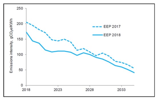
Figure 4.
Future carbon intensities (power plants gate-to-gate) for the UK (estimated in 2017 and 2018) [28].
The main conclusion of Figure 3 and Figure 4 is that LCA databases must be held up-to-date continuously. However, in practice Ecoinvent in SimaPro and Gabi are lagging behind the actual state by approximately 6–8 years. Given the fact that we should reduce by a factor 2 the GHG emissions in the coming 10 years, this delay time must be considered as too long. In contrast, the delay in IEA, E-PRTR, and Association of Issuing Bodies (AIB) [29] databases is only 1 to 2 years.
3.3. Fluctuations Over Time and Time-Related Allocation
3.3.1. Fluctuation Over Time (Short Term)
The production mix in countries varies heavily between day and night (in summer and in winter), but also between periods of wind and no-wind and sun and no-sun. In the near future, when there will be a higher supply percentage of renewable energy, these fluctuations will become more prominent. This issue is mentioned in the ILCD manual [18] (p. 129, Section 6.8.3, note 102):
“Electricity markets are relatively difficult to delimit, given the internationally connected grids. In addition and related to the time-representativeness, it matters whether the named consumer good would be operated only at peak hours (e.g., an electric toothbrush) or continuously (e.g., a fridge) or only during night time at base load (e.g., an electric storage heater)”.
These fluctuations in time have been neglected in most LCA studies. However, in calculations on electric vehicles, where car driving and charging are not spread evenly over the day, the fluctuations in wind and solar energy (i.e., the C-intensity of the country consumption mix of electricity) must be taken into account. Figure 5 shows the strong day-night fluctuations of the C-intensity of the Germany electricity due to wind farms and PV, compared to the low-carbon and stable profile for the French electricity due to its high share of nuclear power [30]. Figure 6 and Figure 7 show, as an example, the carbon intensities in summer and in winter for the UK electricity. The fluctuations in the mix of resources in the UK are given in Figure 8.
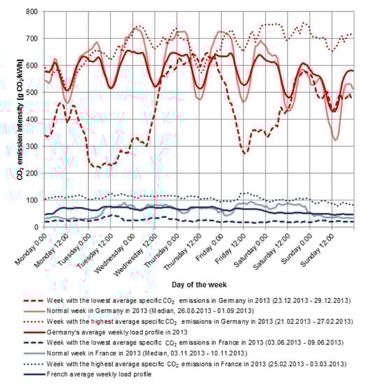
Figure 5.
Carbon intensities of electricity generation in France and Germany in 2013. Source: [30] copyright of the authors.
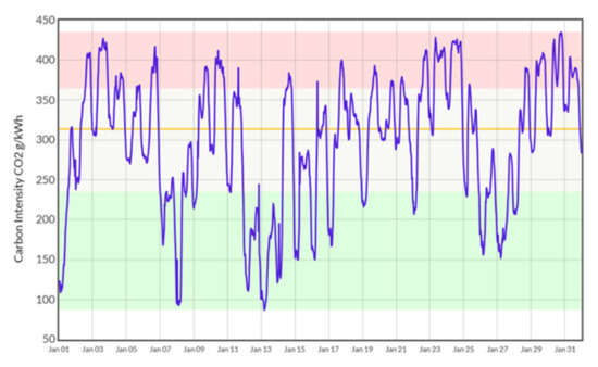
Figure 6.
The UK carbon intensity of electricity production during January 2019. Source: Elexon [31]. Elexon is to be recognized as the source in any reproduction of this material.
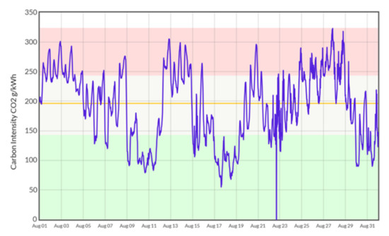
Figure 7.
The UK carbon intensity of electricity production during August 2019. Source: Elexon [31]. Elexon is to be recognized as the source in any reproduction of this material.
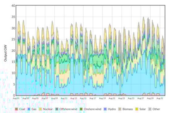
Figure 8.
The source of electricity in the UK during August 2019. Source: Elexon [31]. Elexon is to be recognized as the source in any reproduction of this material.
The conclusion of Figure 5, Figure 6, Figure 7 and Figure 8 is that the yearly average consumption mix may be taken for a 3 shift continuous operation of a manufacturing company. However, the differences over time of the consumption mix should be taken into consideration for all other situations, when the focus is on high accuracy in LCA.
3.3.2. Time-Related Allocation of the Environmental Burden of Windmill and PV Cells
The common practice in LCA is that the eco-burden of construction and maintenance of windmills or PV cells is equally spread over the total production of electricity. However, it remains to be seen if such an approach is realistic for heavy fluctuating power generation profiles in countries with a high share of renewable sources such as wind farms and solar power parks. Should every MJ carry the same burden when there are periods of overproduction (e.g., nights in November where offshore wind power farms might be able to produce more than hinterland needs)? This issue will become more relevant in the near future. At periods when the production of wind farms would have been stopped because of oversupply, the environmental burden of electricity for any storage (in batteries or in hydrogen via electrolysis) may be calculated in LCA in marginal terms, i.e., the share of the emissions of the production and installation of the windmills or PV cells is set to zero. In other words, the environmental footprint of extra produced electricity for local storage is set to zero (or nearly zero). This is time-related allocation on the basis of the marginal (additional) physical flow. A consistent accounting between users of regular and surplus electricity is however strictly required.
This issue of using superfluous production capacity is also touched upon in the GHG protocol (Section 8, subsection ‘Reductions in indirect emissions’) [20]:
“Reductions in indirect emissions (changes in scope 2 or 3 emissions over time) may not always capture the actual emissions reduction accurately. This is because there is not always a direct cause-effect relationship between the activity of the reporting company and the resulting GHG emissions. For example, a reduction in air travel would reduce a company’s scope 3 emissions. This reduction is usually quantified based on an average emission factor of fuel use per passenger. However, how this reduction actually translates into a change in GHG emissions to the atmosphere would depend on a number of factors, including whether another person takes the “empty seat” or whether this unused seat contributes to reduced air traffic over the longer term. Similarly, reductions in scope 2 emissions calculated with an average grid emissions factor may over- or underestimate the actual reduction depending on the nature of the grid”.
This situation of overcapacity is relevant to hydrogen production by electrolysis: the appealing idea is to produce the hydrogen at moments of overcapacity of a wind farm, when the price is low (since the price has only to level with the marginal production costs of the electricity). In LCA the emissions of electricity might similarly be set to zero at such periods when there is a direct cable connection (i.e., physical allocation) to the hydrogen production facility. However, such an approach, considering that marginal “superfluous” electricity does not bear any infrastructure impact, is questionable.
A more general solution, however, would be to apply economic allocation, where the burden of the windmill or the PV cell is spread on the basis of the economic production value of electricity. Such an economic allocation approach would lead to Equation (1):
where:
- a = time-based economic allocated environmental burden per kWh;
- x = yearly average environmental burden of electricity per kWh of a windmill or PV cell (as available in background process databases, e.g., Ecoinvent, GaBi, Idemat, ProBas);
- z(t) = time-based economic allocation factor = ‘actual price per kWh’ divided by the ‘yearly average price per kWh’;
- t = time in discrete steps of 1 h.
3.3.3. Time-Related Allocation of the Environmental Burden of the Electricity Mix at the Grid
There is a subtle difference between the issue of time related allocation of the electricity mix, compared to time related allocation of windmills and PV cells [32]. While time allocation in the case of windmills and PV cells is a matter of ‘fairness’, time allocation of a grid mix is a matter of the actual fluctuation in time of the carbon intensity of electricity (Figure 5, Figure 6 and Figure 7) [33]. For a further explanation of this issue, see Appendix A.
When the actual carbon intensity profile is known, it makes sense (ISO 14044, Section 4.3.4.2) to apply time-related allocation on the basis of the time-related carbon intensity of that electricity mix, see Formula (2):
where:
- a = time-based physical allocated environmental burden per kWh;
- x = yearly average environmental burden of electricity per kWh of the country consumption (or production) mix (as available in background process databases, e.g., Ecoinvent, Gabi, Idemat, ProBas);
- c(t) = time-based physical allocation factor = ‘actual carbon content in kg CO2eq per kWh’ divided by the ‘yearly average carbon content in kg CO2eq per kWh’. Note that this ratio is a mass-based allocation factor;
- t = time in discrete steps of 1 h.
For a further explanation on the above-mentioned formulas, and formulas for the practical situation that the current varies in time (as is the case of Hydrogen production by electrolysis in the 3 different situations of Figure A1), see Appendix A.
3.4. The Guarantee of Origin (GO) and the Residual Mix
The GO discloses the attributes of the electricity supplied to the end-user. In case of renewable origin of the electricity as defined in [23]:
“For the purpose of this Directive […] ‘guarantee of origin’ means an electronic document which has the sole function of providing evidence to a final customer that a given share or quantity of energy was produced from renewable sources. A guarantee of origin can be transferred, independently of the energy to which it relates, from one holder to another”.
The idea of the European Commission is to give energy consumers the choice of buying renewable energy and to choose the source they want to get their energy from. The underlying assumption is that the consumers’ choice will give impetus to the energy transition. A Guarantees of Origin is applied to enable the market-based approach of the GHG protocol. GOs allow users willing to pay a premium for a given type of production to valorize it. GOs are traded independently from the electricity trade.
The certification is regulated by the European Energy Certification System (EECS) and monitored by EU Member states through their national Issuing Bodies. Double counting is prevented by the Issuing Body which ensures that Guarantees of Origin are used only once. ‘Country Residual Mix’ in the EU-27 is the country consumption mix where the GO deliveries have been subtracted. It is the mix corresponding to the untracked consumption of electricity in a country [34].
The system of GOs, however, is still under development. The system suffers at the moment from the fact that the country export and import of GOs does not correspond with the export and import of electricity [35,36,37]. The system has still 3 fundamental flaws: (1) Austria, Switzerland, and the Netherlands have 100% tracing (‘full disclosure’), but other countries must do the same to get the import and export data right; (2) a working group within the AIB has developed in 2020 a new calculation system [38], but there are still administrative problems to be resolved with regard to time delays of several months between production of renewable electricity and the trading of the corresponding GOs; (3) at this moment, you can get solar power from the supplier when there is no sun; Vattenvall and Microsoft are solving this issue by an administrative system that monitors the production mix at an hourly basis [39], which is a first pilot in the Energy Tag project to regain trust of clients. By getting the registration right on an hourly basis, the current problem is solved that companies can buy electricity from coal and compensate that with GOs from renewable sources (which is by far the cheapest way to lower the administrative CO2 emissions, since the price of a GO is a factor 15–200 lower than the price of electricity [40]).
Therefore, the flaws are expected to be repaired in the coming years. That GOs are already used in corporate communication supports the urgency of progress to be made. The GHG Protocol Scope 2 Guidance [7] (p. 7):
“The Corporate Standard does not address potential double counting between consumers of emissions associated with green power instruments.” And “implementing a credible and robust system for GHG emission… would require that only one consumer reports the emissions from a given quantity of generation”.
It can be considered to apply a specific GO in LCA, provided that: (1) the GO is bought from the same production field as the electricity (‘a bundled GO’), and (2) the required storage system is taken into account (range 75–85% for pumped hydroelectric storage [41]). The issue is still under discussion [42], and needs further specification. However, it does not make sense to use the Residual Electricity in LCA since it is highly inaccurate. For a further explanation, see https://www.ecocostsvalue.com/lca/gos-and-recs-in-lca/ (accessed on 20 April 2021).
3.5. Selection of Midpoints or Endpoint Systems: The Specific Case of Nuclear Energy
Given the wide varieties of systems that generate electricity, the issue of selecting a mid- or end-point system (e.g., carbon footprint or eco-costs, ReCiPe, Environmental Footprint (EF)-single score) for decision taking becomes prominent, since the choice of a midpoint or end-point system influences the decision in LCA benchmarking.
It is common practice to limit an LCA to Global Warming Potential (GWP) impact, which does not reflect any other effects on the environment. However, ISO 14044 Section 4.4.2.2.1 asks for a careful selection of impact categories:
“The selection of impact categories, category indicators and characterization models shall be both justified and consistent with the goal and scope of the LCA. The selection of impact categories shall reflect a comprehensive set of environmental issues related to the product system being studied, taking the goal and scope into consideration.”
A rather controversial issue is the quantification of the environmental impact and risk associated with nuclear power, and the comparison to its benefits of low CO2 emissions. The issue becomes clear with regard to the Well-To-Wheels benchmarking study of Figure 1: in countries with a lot of nuclear power like France (and Belgium), there is an enormous advantage of electric vehicles compared to internal combustion engine vehicles in terms of GHG emissions. Figure 1 might even be a bit misleading: France and Sweden score both low, but from an environmental point of view there is a big difference between France (73.3% nuclear energy, 18.5% renewable) and Sweden (42.7% nuclear energy, 54.1% renewable) [43]. The awkward question, however, is how to compare nuclear power with CO2 emissions from fossil fuels in LCA. One approach is to avoid this comparison and stop at the level of midpoints or even of data inventory. For example, in the yearly reports published by AIB, greenhouse gas emissions per kWh of produced electricity and corresponding amount of highly active radioactive waste are shown without any attempt of benchmarking [29]. If such an attempt is made, there are two questions first to be answered: (1) in which impact category is nuclear energy counted? (2) what is the impact factor of nuclear (characterization factor, and the factors for normalization and weighting)?
In damage-based single score methods (e.g., ReCiPe), the question arises on the issue of the risk of damage, which is virtually impossible to calculate for the use of uranium. In ReCiPe 2016 V1.1 [44], the nuclear damage risk is not modeled: the score for uranium is determined by its resource scarcity in the group of minerals, which results in a (relative) very low score per MJ of electricity.
In EF V3.0 [45], the damage risk is not modeled as well: the issue is resolved by grouping uranium in the category of energy carriers (characterization factor in MJ of the embedded energy), so that nuclear fuels are linked to the depletion factors for fossil fuels, leading to a much higher score than in ReCiPe.
In the eco-costs 2017 V1.6 system, nuclear energy is quantified by its prevention costs (in contradiction to damage costs), in compliance with ISO 14008:2019. In the eco-costs system, the prevention costs are modelled by the costs of replacement of uranium powered electrical power plants, calculated per MJe [46]. Note that the debate on the risk of uranium is avoided in the eco-costs system, and replaced by the assumption that in the long run, second and third generation nuclear power is not a sustainable solution: (1) its vulnerability for sabotage by extremists, (2) its disposal of hazardous waste, (3) it cannot cope with the operational flexibility that is needed to compensate the fluctuations of wind and solar power [47], and (4) its financial risks [48].
The choice of which approach to follow for including the impact of nuclear power is basically a subjective decision which has to be made at organizational level (government, company, NGO, …).
Figure 9 depicts the environmental burden of the electricity consumption mix for European countries as a percentage of the ENTSO-E score for the following indicators: (1) carbon footprint, including supply chain [11], (2) ReCiPe 2016 Endpoint ‘Hierarchist’, in combination with medium voltage LCIs from Ecoinvent (EI), (3) EF single score in combination with medium voltage LCIs from PEF (GaBi), (4) Eco-costs2017 in combination with medium voltage LCIs from EI, and (5) EF single score in combination with medium voltage LCIs from EI.
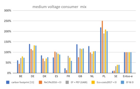
Figure 9.
The endpoint scores of the electricity consumption mix for European countries. The scores are expressed as a percentage of the score for the European Network of Transmission System Operators for Electricity (ENTSO-E). For data, see Table 2.
The differences in endpoint scores for each country, predominantly caused by the share of nuclear energy, have practical implications in LCA benchmarking. An example is an LCA on cross-border commuting with BEVs [30]. The conclusion that French–German commuting BEVs should load their cars in France, holds under every endpoint system. However, for French–Belgian commuting BEVs, the conclusion depends on the choice of endpoint and LCI database, see Figure 9.
Note that there is no single truth in single endpoint indicator systems [49], since such a system reflects a set of values and assumptions, but it is generally acknowledged that single score systems are needed in LCA benchmarking [50]. A well-documented scientific scoring system is always better than a set of many midpoint scores of which one or two are selected on the basis of a personal, subjective, point of view [51].
In ReCiPe, nuclear energy has a very low factor in the normalization and weighting calculation step (which is an explanation for the low scores in FR and SE in Figure 9). It is a typical example of the problems that are related to normalization and weighting. In recent papers, the systems for normalization and weighting have been scrutinized [51,52] but the applied systems in this paper are the best we have at the moment. The eco-costs system is different: it has no normalization and weighting sets in the calculation [53], but is built on the different paradigm of prevention costs [54].
From the bars in Figure 9 it can be concluded that scores of a country, relative to the ENTSO-E average, may vary by 30% for the different combinations of LCI database with single endpoint score system, apart from the fact that nuclear power is neglected in ReCiPe. As such, the differences are only important when they lead to different decisions (e.g., on the choice of a manufacturing facility). The ranking of countries is given in Table 2.
Table 2.
The ranked endpoint scores for European countries as a percentage of the ENTSO-E scores (carbon footprint from [11], PEF data from 2013, Ecoinvent (EI) data from 2014.)
With regard to Table 2, there are 3 comments:
- In endpoint systems there is no single truth: ReCiPe is based on damage, EF is primarily based on normalization and weighting by a hybrid system of public opinion and expert panels, and eco-costs is based on prevention (i.e., 3 different approaches to weighting in situations of trade-off). It is a coincidence that the eco-costs system and EF have nearly the same ranking (only the positions of DK, FR, and BE switch);
- Data of countries can change rapidly: in the period 2013–2016, the carbon intensity improved in GB by 38%, in DK by 34%, where the ENTSO-E data improved by 11% (see also Figure 3). Therefore, the ranking of countries changes quickly and might be affected by the age of the LCI database;
- Common practice in LCA is to take one database and one endpoint system as the basis for a comparison. Combining two different databases in one benchmark study is not advised, since it adds an extra level of inaccuracy, especially for country scores. On the other hand, it is advised to calculate the LCA results with two or more Life Cycle Impact Assessments (LCIA) methods in order to assess the robustness of the conclusions.
4. Discussion
The results of the analyses of this paper are discussed for the 5 research questions (RQs) as given in Section 1:
- RQ 1. What is the uncertainty in applying LCI data from existing leading databases?
The yearly average data for electricity of countries in the leading databases are not very accurate. The differences between the databases for the carbon intensity is 20–30% for the following 9 European countries: BE, DE, DK, ES, FR, GB, NL, PL, SE (see Table 1). The reason for the inaccuracy is that the LCI databases—Ecoinvent, PEF (GaBi), and ELCD—are based on calculations by parameterization, rather than direct measurements. The general setup of the calculations is well documented, however, the details on the parameterization are not provided. It is not possible to give an assertion on which database is the best.
- RQ 2. What is the effect of the fact that the LCI data are in practice 4–8 years old on average?
In the EU, the average carbon intensity declined by 25% in the period 2006–2016 (Figure 3). During the short period of 3 years in 2013–2016, the UK improved by 38% and DK by 34%. That means that lagging behind 4–8 years in data for electricity is simply too much.
- RQ 3. How to deal with the fluctuations over time of the carbon intensity of electricity and time-related allocation on a time scale of 1 h?
The variations of carbon intensity over time will become quite heavy with the increase of the share of wind and solar power. That can be observed in Germany, where the carbon intensity varies from 250 to 730 g CO2/kWh, see Figure 5. The same can be observed in the UK, where it varies from 100 to 440 g CO2/kWh in winter (Figure 6), and from 100 to 300 g CO2/kWh in summer (Figure 7). Especially in Well-to-Wheel calculations on BEVs, and FCVs and in other applications of hydrogen production, these fluctuations will govern LCA calculations. To become accurate in LCA, the actual, time-dependent, carbon intensity must be taken, instead of the average, see Formula (2). For electricity from windmills and PV cells it is advised to apply economic allocation, see Formula (1) and Appendix A.
- RQ 4. When does it make sense to use in LCA electricity Guarantee of Origin and residual mix, and when the consumption mix?
GOs might be applied in LCA, provided that: (1) the GO is purchased from the same production field as the electricity, and (2) the required storage system is taken into account. Residual mix in LCA shall not be used until sound data are available (i.e., 100% tracing, i.e., ‘full disclosure’, at an hourly basis in the countries that are involved). However, this will take at least 5–10 years.
- RQ 5. How to deal with nuclear power in relation to greenhouse gas emissions (the issue of comparing ‘apples with oranges’ by the selection of midpoints and endpoints in LCA)?
Risks from nuclear power and climate impact belong to two different impact categories and their comparison is highly controversial. The only way to deal with this kind of trade-off issues is to apply one of the single indicator endpoint systems (e.g., ReCiPe, EF, eco-costs). However, that introduces two aspects that add to inaccuracy: (1) the inaccuracy of other emissions than GHG emissions (like SO2, NO2, fine dust, et cetera) in the current main LCI databases Ecoinvent, ELCD, and PEF, (2) the different approaches to weighting in each endpoint system. In the ReCiPe H system, the end score for nuclear power is negligible compared to fossil fuel power, in contrast to EF and eco-costs, see Figure 9. This is relevant for ranking countries on the score of the consumption mix electricity, see Table 2.
5. Conclusions
- In ex-post generic LCAs on battery electric vehicle systems and electrolytic hydrogen systems, the use of the country consumption mix (in contrast to the EU grid mix) goes hand in hand with high inaccuracies, see Table 1. Sensitivities analyses might help assessing the robustness/variability of the conclusions.
- The residual mix should not be applied because of its huge inaccuracies. Only ‘bundled GOs’ should be used in LCA, taking into account the required electricity storage.
- Ex-ante LCA studies should refrain from using the country consumption mix (ex-post) data from databases, but should always have an assumed future technical mix of electricity (percent wind power, solar power, etcetera, and fossil fuels), and have a sensitivity analysis on it. Note that the vast majority of published LCA studies are ex-ante, since they aim at mitigation of environmental pollution by redesigning the product-service systems for the future.
- New time-dependent allocation rules are needed in LCA benchmarking of modern technologies like battery electric vehicle systems and hydrogen fuel cell vehicle systems, to cope with the fact that these new technologies are designed to partly use electricity at moments of overproduction of, e.g., wind farms.
- There is a rather urgent need for a new electricity database, that is built on bottom-up data like the European Pollutant Release and Transfer Register (E-PRTR) [26]. Such a database can provide an accurate assessment of the emissions from the production mix per country. Combined with import and export data from ENTSO-E, country consumption mix data can be calculated which are not older than 2 years. In such a way, the LCI lists will be much more accurate, since they are based on measurements, and calculations are based on the locally applied technologies and specific feedstock data. The database should be open access and transparent.
Further research is needed on the following issues:
- (1)
- The electricity calculation rules in the PEF project should be reconsidered;
- (2)
- The GHG protocol should distinguish between bundled and unbundled RECs and GOs;
- (3)
- The EU should stimulate ‘full disclosure’ systems of electricity in member states;
- (4)
- A dataset for electricity that is based on the actual emissions in the EU (E-PRTR [26]), the USA (eGRID [55]) and Canada (APEI [56]) has been calculated by the Delft University of Technology [57], but further developments are needed.
Author Contributions
Ideation, R.O.; conceptualization and original draft preparation, J.V.; data analysis, R.O., N.S., and J.V.; writing—review and editing, R.O., N.S., and J.V. All authors have read and agreed to the published version of the manuscript.
Funding
This research received no external funding.
Informed Consent Statement
Not applicable.
Data Availability Statement
Data sharing not applicable.
Acknowledgments
The authors thank Air Liquide who made this study possible.
Conflicts of Interest
The authors declare no conflict of interest.
Appendix A. The Basics of Time-Related Allocation; Production of Hydrogen by Electrolysis as an Example
Allocation in LCA is defined in ISO 14044 as: “Partitioning the input or output flows of a process or a product system between the product system under study and one or more other product systems”.
Practical examples on output flows are:
- The products of a sheep: which part of the eco-burden of a sheep (cradle-to-gate of its primary products) is allocated to the wool and which part is allocated to the meat (and the leather)?
- The products of a tree: which part of the eco-burden of a harvested tree (cradle-to gate of its primary products) is allocated to the wooden beams, and which part to the wood chips (and saw dust)?
As a result that there is no obvious solution to many practical allocation problems, ISO 14044 leaves a large degree of freedom, and can be interpreted in many ways. One of the issues is that physical allocation (i.e., allocation based on mass, volume, heat content, or any other physical unit) can be considered unfair for users of low-valued by-products. To prevent this unfairness, it is quite common to base the allocation on the price of the product, the co-products, and the by-products.
Although it is not common in LCA to apply time-based allocation, it is the logical way to resolve the issue on how to calculate the environmental burden of electricity, given the complex variability of the electricity mix in countries (Figure 4, Figure 5, Figure 6 and Figure 7) and given the fact that standard LCI databases provide only information on yearly averages. There are two different solutions to cope with two different problems:
- Multiplying the yearly average environmental burden of the electricity of a windmill (or PV cell), as provided in databases on background processes, with an economic allocation factor (i.e., the ‘actual price per kWh’ divided by the ‘yearly average price per kWh’).The reason to apply economic allocation is that it is considered unfair that the low-valued electricity at moments of overproduction, or nearly overproduction, carry the same eco-burden than high-valued electricity. Note that such an allocation factor is smaller than 1 in periods where the demand of electricity is low, and higher than 1 when the demand of electricity is high.
- Multiplying the yearly average environmental burden of the electricity mix in a country, as provided in databases on background processes, with a physical allocation factor (i.e., the ‘actual carbon content per kWh’ divided by the ‘yearly average carbon content per kWh’).Note that the actual carbon content ratio provides a better allocation factor for the country electricity mix than the price ratio, since the price and the carbon content have a weak relationship because of fluctuations in the feedstock prices of fossil fuels in the electricity mix.
The above reasoning leads to Formulas (1) and (2) in Section 3.3 for the situation of a constant current over the calculated time interval, e.g., a loading station for a BEV.
However, Formulas 1 and 2 cannot cope with situations where the current during the calculated time interval is fluctuating.
Such situations occur during the production of green hydrogen by electrolysis: since the price of electricity is a major element in the price of green hydrogen, it is common sense to possibly produce the hydrogen at moments of low prices. This leads to a situation where the hydrogen production plant operates with a variable current (load factor) in an “open system”, see Figure A1. This leads to Formula (A1):
where:
- a = time-based economic allocated environmental burden per kWh;
- x = yearly average environmental burden of electricity per kWh of a windmill or PV cell (as available in background process databases, e.g., Ecoinvent, GaBi, Idemat, ProBas);
- y(t) = , where electricity(t) indicate the power in kWh in function of the time t;
- z(t) = time-based economic allocation factor = ‘actual price per kWh’ divided by the ‘yearly average price per kWh’;
- t = time in discrete steps of 1 h.
When the Hydrogen plant is not directly connected to a windfarm, but just to the grid, see Figure A1 (‘grey Hydrogen from electrolysis’), Formula (A2) should be applied:
where:
- a = time-based physical allocated environmental burden per kWh;
- x = yearly average environmental burden of electricity per kWh of the country consumer (or production) mix (as available in background process databases, e.g., Ecoinvent, Gabi, Idemat, ProBas);
- y(t) = , where electricity(t) indicate the power in kWh in function of the time t;
- c(t) = time-based physical allocation factor = ‘actual carbon content in kg CO2eq/ kWh’ divided by the ‘yearly average carbon content in kg CO2eq/ kWh’;
- t = time in discrete steps of 1 h.
In practical situations of hydrogen production by electrolysis, the electricity for the production will be characterized by Formula (A1) for a certain period of time and formula (4) for the rest of the time. See Figure A1 “open system”. Note that the above formulas for hydrogen production are highly relevant for the so-called ‘recycling of CO2′ (converting CO2 to CH4 or other hydrocarbons), e.g., from flue gas [58], which can even lead to a negative carbon footprint in the case of biogenic CO2.

Figure A1.
Three system configurations (“closed system”, “open system”, “via grid”).
References
- Schuller, A.; Stuart, C. From Cradle to Grave: E-Mobility and the Energy Transition; Addendum for Italy, the United Kingdom, Spain and the European Union to Le Véhicule Électrique dans la Transition Écologique en France; Carbon 4: Paris, France, 2018. [Google Scholar]
- EUR-Lex. Available online: https://eur-lex.europa.eu/legal-content/EN/TXT/?qid=1576150542719&uri=COM%3A2019%3A640%3AFIN (accessed on 22 April 2021).
- Hydrogen-Scaling-Up Hydrogen-Council. Hydrogen Scaling Up. A Sustainable Pathway for the Global Energy Transition; Hydrogen Council: Brussels, Belgium, 2018; Available online: https://hydrogencouncil.com/wp-content/uploads/2017/11/Hydrogen-scaling-up-Hydrogen-Council.pdf (accessed on 26 April 2021).
- Koj, J.C.; Wulf, C.; Schreiber, A. Site-Dependent Environmental Impacts of Industrial Hydrogen Production by Alkaline Water Electrolysis. Energies 2017, 10, 860. [Google Scholar] [CrossRef]
- Bodineau, L. Analyse du Cycle de Vie Relative à l’Hydrogène–Production d’Hydrogène et Usage en Mobilité Légère; ADEME: Angers, France, 2020. [Google Scholar]
- Valente, A.; Iribarren, D.; Dufour, J. Harmonized life-cycle global warming impact of renewable hydrogen. J. Clean. Prod. 2017, 149, 762–772. [Google Scholar] [CrossRef]
- Sotos, M. GHG Protocol Scope 2 Guidance. In GHG Protocol; World Resources Institute: Washington, DC, USA, 2015; ISBN 978-1-56973-850-4. [Google Scholar]
- Cucurachi, S.; van der Giesen, C.; Guinee, J. Ex-ante LCA of Emerging Technologies. In Proceedings of the 25th CIRP Life Cycle Engineering (LCE) Conference, Copenhagen, Denmark, 30 April–2 May 2018. [Google Scholar]
- Garraín, D.; Fazio, S.; de la Rúa, C.; Recchioni, M.; Lechón, J.; Mathieux, F. Background qualitative analysis of the European reference life cycle database (ELCD) energy datasets–part II: Electricity datasets. SpringerPlus 2015, 4, 30. [Google Scholar] [CrossRef][Green Version]
- Lozanovski, A.; Schuller, O.; Faltenbacher, M. Guidance Document for performing LCAs on Fuel Cells and H2 Technologies. Deliverable D3.3–2011-09-30 Final Guidance Document. Available online: http://hytechcycling.eu/wp-content/uploads/FC-Guidance-Document.pdf (accessed on 26 April 2021).
- Moro, A.; Lonzo, L. Electricity carbon intensity in European Member States: Impacts on GHG emissions of electric vehicles. Transp. Res. D 2018, 64, 5–14. [Google Scholar] [CrossRef] [PubMed]
- Peters, J.F.; Baumann, M.; Zimmermann, B.; Braun, J.; Weil, M. The environmental impact of Li-Ion batteries and the role of key parameters-A review. Renew. Sustain. Energy Rev. 2016, 67, 491–506. [Google Scholar] [CrossRef]
- Kawamoto, R.; Mochizuki, H.; Moriguchi, Y.; Nakano, T.; Motohashi, M.; Sakai, Y.; Inaba, A. Estimation of CO2 Emissions of Internal Combustion Engine Vehicle and Battery Electric Vehicle Using LCA. Sustainability 2019, 11, 2690. [Google Scholar] [CrossRef]
- Edwards, R.; Hass, H.; Larivé, J.F.; Lonza, L.; Maas, H.; Rickeard, D. Well-to Wheels Analysis of Future Automotive Fuels and Powertrains in the European Context. In JRC Technical Reports; Godwin, S., Hamje, H., Krasenbrink, A., Nelson, R., Rose, K.D., Eds.; Publications Office of the European Union: Luxemburg, 2014; ISBN 978-92-79-33887-8. [Google Scholar]
- Frischknecht, R.; Bollens, U.; Bosshart, S.; Ciot, M.; Ciseri, L.; Doka, G.; Dones, R.; Gantner, U.; Hischier, R.; Martin, A. Ökoinventare von Energiesystemen: Grundlagen für den ökologischen Vergleich von Energiesystemen und den Einbezug von Energiesystemen in Ökobilanzen für die Schweiz, 3rd ed.; Bundesamt für Energiewirtschaft (BEW): Zurich, Switzerland, 1996. [Google Scholar]
- Itten, R.; Frischknecht, R.; Stucki, M. Life Cycle Inventories of Electricity Mixes and Grid; Treeze: Uster, Switzerland, 2014. [Google Scholar]
- ElectricityMap|Live CO2 Emissions of Electricity Consumption. Available online: https://www.electricitymap.org (accessed on 29 April 2021).
- General guide for Life Cycle Assessment–detailed guidance. In ILCD Handbook, 1st ed.; European Commission–JRC: Ispra, Italy, 2010.
- Specification for the assessment of the life cycle greenhouse gas emissions of goods and services. In PAS 2050:2011; BSI: London, UK, 2011.
- A Corporate Accounting and Reporting Standard. In The Greenhouse Gas Protocol; World Resources Institute and World Business Council for Sustainable Development: Washington, DC, USA, 2004.
- European Commission. PEFCR Guidance Document - Guidance for the development of Product Environmental Footprint Category Rules (PEFCRs). In PEFCR Guidance Document; Version 6.3; European Commission: Brussels, Belgium, 2017; Available online: https://ec.europa.eu/environment/eussd/smgp/pdf/PEFCR_guidance_v6.3 (accessed on 25 April 2020).
- Zampori, L.; Pant, R. Suggestions for Updating the Product Environmental Footprint (PEF) Method; Publications Office of the European Union: Luxemburg, 2019; ISBN 978-92-76-00654-1. [Google Scholar]
- Renewable Energy Directive II of the European Parliament and the Council of the European Union; Publications Office of the European Union: Luxemburg, 2018.
- Malins, C. What Does it Means to Be a Renewable Electron? The International Council on Clean Transportation (ICCT): Washington, DC, USA, 2019. [Google Scholar]
- Turconi, R.; Boldrin, A.; Astrup, T. Life cycle assessment (LCA) of electricity generation technologies: Overview, comparability and limitations. Renew. Sustain. Energy Rev. 2013, 28, 555–565. [Google Scholar] [CrossRef]
- E-PRTR Database. Available online: https://prtr.eea.europa.eu (accessed on 25 April 2020).
- EEA Database. Available online: https://www.eea.europa.eu/data-and-maps/indicators/overview-of-the-electricity-production-2/assessment-4 (accessed on 25 April 2020).
- Updated Energy and Emission Projection 2018; Department for Business, Energy & Industrial Strategy-Government of the United Kingdom: London, UK, 2019.
- Association of Issuing Bodies. European Residual Mix|AIB. Available online: https://www.aib-net.org/facts/european-residual-mix (accessed on 25 February 2021).
- Ensslen, A.; Schücking, M.; Jochem, P.; Steffens, H.; Fichtner, W.; Wollersheim, O.; Stella, K. Empirical carbon dioxide emissions of electric vehicles in a French-German commuter fleet test. J. Clean. Prod. 2017, 142, 263–278. [Google Scholar] [CrossRef]
- Fuel Mix Archive. Available online: http://electricityinfo.org/fuel-mix-archive/#data (accessed on 25 December 2019).
- Onishi, V.C.; Antunes, C.H.; Trovão, J.P.F. Optimal Energy and Reserve Market Management in Renewable Microgrid-PEVs Parking Lot Systems: V2G, Demand Response and Sustainability Costs. Energies 2020, 13, 1884. [Google Scholar] [CrossRef]
- Noussan, M.; Roberto, R.; Nastasi, B. Performance Indicators of Electricity Generation at Country Level—The Case of Italy. Energies 2018, 11, 650. [Google Scholar] [CrossRef]
- European Residual Mix for the Calendar Year 2018. Available online: https://www.aib-net.org/facts/european-residual-mix (accessed on 25 April 2020).
- Hamburger, A. Is Guarantee of Origin really an effective energy policy tool in Europe? A critical approach. Soc. Econ. 2019, 41, 487–507. [Google Scholar] [CrossRef]
- Hufen, J. Cheat Electricity? The Political Economy of Green Electricity Delivery on the Dutch Market for households and small business. Sustainability 2017, 9, 16. [Google Scholar] [CrossRef]
- Jansen, J. Does the EU Renewable Energy Sector Still need a Guarantees of Origin Market? CEPS Policy Insights: Brussels, Belgium, 2017. [Google Scholar]
- Kuronen, A.; Lehtovaara, M.; Jakobsson, S. Issuance Based Residual Mix Calculation Methodology 2020. Available online: https://www.aib-net.org/facts/european-residual-mix (accessed on 25 January 2021).
- Vattenfall, Press and Media. Vattenfall to Deliver Renewable Energy 24/7 to Microsoft’s Swedish Datacenter. Available online: https://group.vattenfall.com/press-and-media/pressreleases/2020/vattenfall-to-deliver-renewable-energy-247-to-microsofts-swedish-datacenters (accessed on 25 January 2021).
- ECOHZ. The European Market For Renewable Energy Reaches New Heights—ECHZ. Available online: https://www.ecohz.com/press-releases/the-european-market-for-renewable-energy-reaches-new-heights (accessed on 25 February 2021).
- World Energy Council. ES_Five_Steps_to_Energy_Storage_-_English. Available online: https://www.worldenergy.org/assets/downloads/ES_Five_Steps_to_Energy_Storage_-_ENGLISH.pdf (accessed on 25 February 2021).
- Brander, M.; Gillenwater, M.; Ascu, F. Creative accounting: A critical perspective on the market-based method for reporting purchased electricity (scope 2) emissions. Energy Policy 2018, 112, 29–33. [Google Scholar] [CrossRef]
- Statistical Factsheet 2013; European Network of Transmission System Operators for Electricity: Brussels, Belgium, 2014.
- Huijbregts, M.; Steinmann, Z.; Elshout, P.; Stam, G.; Verones, F.; Vieira, M.; Van Zelm, R. ReCiPe2016: A harmonised life cycle impact assessment method at midpoint and endpoint level. Int. J. Life Cycle Assess. 2016, 22, 138–147. [Google Scholar] [CrossRef]
- Fazio, S.; Castellani, V.; Sala, S.; Schau, E.M.; Secchi, M.; Zampori, L.; Diaconu, E. Supporting Information to the Characterisation Factors of Recommended EF Life Cycle Impact Assessment Method; European Commission–JRC: Ispra, Italy, 2018. [Google Scholar]
- Eco-Costs of Energy. Available online: https://www.ecocostsvalue.com/EVR/model/theory/subject/2-eco-costs.html (accessed on 25 April 2020).
- Gonzalez-Salazar, M.A.; Trevor Kirsten, T.; Prchlik, L. Review of the operational flexibility and emissions of gas- and coal-fired power plants in a future with growing renewables. Renew. Sustain. Energy Rev. 2018, 82, 1497–1513. [Google Scholar] [CrossRef]
- Managing the Financial Risk Associated with the Financing of New Nuclear Power Plant Projects. In IAEA Nuclear Energy Series No. NG-T-4.6; International Atomic Energy Agency: Vienna, Austria, 2017.
- Wulf, C.; Zapp, P.; Schreiber, A.; Marx, J.; Schlör, H. Lessons Learned from a Life Cycle Sustainability Assessment of Rare Earth Permanent Magnets. J. Ind. Ecol. 2017, 21, 1578–1590. [Google Scholar] [CrossRef]
- Sala, S.; Cerutti, A.K.; Pant, R. Development of a weighting approach for the Environmental Footprint. In JRC Technical Reports; Publications Office of the European Union: Luxemburg, 2018; ISBN 978-92-79-68042-7. [Google Scholar]
- Prado, V.; Cinelli, M.; Ter Haar, S.; Ravikumar, D.; Heijungs, R.; Guinée, J.; Seager, P. Sensitivity to weighting in life cycle impact assessment (LCIA). Int. J. Life Cycle Assess. 2020, 25, 2393–2406. [Google Scholar] [CrossRef]
- Kim, J.; Bae, J.; Yang, Y.; Suh, S. The Importance of Normalization References in Interpreting Life Cycle Assessment Results. J. Ind. Ecol. 2013, 17, 385–395. [Google Scholar] [CrossRef]
- Eco-Costs—Wikipedia. Available online: https://en.wikipedia.org/wiki/Eco-costs (accessed on 25 April 2020).
- Bernier, E.; Maréchal, F.; Samson, R. Life cycle optimization of energy-intensive processes using eco-costs. Int. J. Life Cycle Assess. 2013, 18, 1747–1761. [Google Scholar] [CrossRef]
- Emissions & Generation Resource Integrated Database (eGRID). Available online: https://www.epa.gov/egrid (accessed on 25 April 2021).
- Government of Canada. APEI_Tables_Canada_Province_Territ. Available online: http://data.ec.gc.ca/data/substances/monitor/canada-s-air-pollutant-emissions-inventory/APEI_Tables_Canada_Provinces_Territories/?lang=en (accessed on 25 April 2021).
- Delft University of Technology. Data—Eco Cost Value. Available online: https://www.ecocostsvalue.com/data/ (accessed on 25 April 2021).
- Castellani, B.; Rinaldi, S.; Morini, E.; Nastasi, B.; Rossi, F. Flue gas treatment by power-to-gas integration for methane and ammonia synthesis–Energy and environmental analysis. Energy Convers. Manag. 2018, 171, 626–634. [Google Scholar] [CrossRef]
Publisher’s Note: MDPI stays neutral with regard to jurisdictional claims in published maps and institutional affiliations. |
© 2021 by the authors. Licensee MDPI, Basel, Switzerland. This article is an open access article distributed under the terms and conditions of the Creative Commons Attribution (CC BY) license (https://creativecommons.org/licenses/by/4.0/).