Synthesis and Feature Selection-Supported Validation of Multidimensional Driving Cycles

Abstract

This paper presents the synthesis and validation of multidimensional driving cycles represented by vehicle velocity, vehicle acceleration, and road slope profiles. For this purpose, a rich set of city bus driving cycles has been recorded. First, a Markov chain model is established based on velocity, acceleration, road slope and road slope time derivative states. Next, a large set of synthetic driving cycles is generated by using a corresponding 8D transition probability matrix, which is implemented in a sparse form based on a dictionary of keys to improve computational efficiency and reduce memory requirements. In support of synthetic driving cycles validation, a number of time- and frequency-domain statistical features are considered, including unique cross-correlation velocity–acceleration–road slope indicators. To predict fuel consumption related to synthetic driving cycles, an accurate neural network model is introduced which uses a fixed 3D histogram of counted discrete velocity, acceleration, and road slope inputs. The significance of each nominated statistical feature and its impact on fuel consumption is revealed by means of linear regression modelling and least absolute shrinkage and selection operator (LASSO) feature selection method. A model having only several most significant features as inputs and fuel consumption as output is proposed to be used for unambiguous single-criterion validation of synthetic driving cycles with respect to recorded ones. Finally, the proposed validation approach is verified against a widely used method relying on minimization of statistical feature deviations with respect to true values. The results point out that, by applying the proposed synthesis and validation method, it is possible to extract most representative synthetic driving cycles in a straightforward and computationally efficient way. The main anticipated applications include various simulation-based analyses that require representative synthetic driving cycles and/or accurate vehicle energy consumption predictions.

1. Introduction

Vehicle energy consumption and greenhouse gas emissions strongly depend on the driving cycle, as well as on vehicle characteristics, weather conditions, fuel type, and load of auxiliary devices [1,2,3]. The driving cycle is usually defined by a vehicle speed vs. time profile [4,5], which to some extent implicitly contains a driving pattern related to driver’s behaviour (e.g., driving aggressiveness) and driving conditions (road type, road slope, traffic conditions, etc.) [6,7]. Driving cycles used for the purpose of vehicle design and testing should represent actual driving behaviours and road/traffic conditions [8]. Although the certified driving cycles, such as World-wide harmonized Light duty Test Cycles (WLTC) and New European Driving Cycle (NEDC) [9], are routinely and successfully used in standardised laboratory tests for assessment of fuel economy and emissions, they do not faithfully represent real driving conditions [5,10]. Therefore, a significant research effort has been devoted to development of methods for driving cycle synthesis from a large set of recorded real-world driving data. Commonly, micro-trip concatenation [11,12] and Markov chain methods are employed [13,14,15,16]. Since a very large number of different synthetic driving cycles can be generated in this way, the question remains how to assess their representativeness, i.e., which validation method and related driving cycle features should be used to extract a single or a couple of the most representative driving cycles.

1.1. Background

The state-of-the-art commonly involves Markov chain method [17,18,19,20], which can be considered as an extension of finite state machine (FSM) [21], with belonging transitions between states being stochastic (i.e., described by probability distributions) and dependent only on the current state, rather than deterministic and input-based. The main advantage of Markov chain method is related to flexibility in generating unlimited number of synthetic driving cycles in terms of arbitrary time duration and total travelled distance [22]. Typically, the Markov chain states are selected to include the vehicle velocity and acceleration [13,17,22]. However, in general, the synthesis should also account for the road slope effect to improve the accuracy and reliability of fuel economy and emissions tests [16,23]. Since direct measurement of road slope is often not available, it should be reconstructed from raw global positioning system (GPS) data [23,24]. The traditional way of expressing the Markov chain transition probability matrix (TPM) in the form of the N-dimensional array (i.e., tensor) [18,19,20] leads to a high-dimensional problem in the case of including the road slope state, which can be hard to solve due to excessive demands on computer memory and computational power. This issue can be overcome by applying sparse implementation of TPM based on dictionaries of keys, as outlined recently in [24,25].

Synthetic driving cycle validation approaches are usually based on utilization of a set of subjectively selected, vehicle-independent statistical features (typically related to vehicle velocity, acceleration, number of stops, etc.) [19,22,26]. To avoid multi-criteria validation, a unique lumped performance indicator is often derived from multiple statistical features, e.g., a sum of relative deviations from true feature values [20]. However, it should be kept in mind here that not all features have the same relevance from the perspective of driving cycle representativeness. Alternatively, the unique performance indicator can be based on vehicle-dependent specific energy consumption [27], or on matching speed-acceleration frequency distributions (SAFD) of synthetic and recorded driving cycles [3,5]. The main disadvantage of these approaches is that they do not consider comprehensive feature space and thus do not guarantee an adequate degree of driving cycle representativeness with respects to all statistical features. For example, by neglecting the frequency response features, the resulting velocity and road slope profiles may deviate from the recorded patterns in terms of number and duration of vehicle stoppings and the frequency of road slope variations. Therefore, cross-correlation features quantifying interdependence between velocity, acceleration, and road slope should be considered for more comprehensive validation.

The question also remains on how to determine the degree of relevance of each feature when there are many candidates. To answer this question, a special attention should be paid to machine learning methods or, more specifically, feature selection techniques. Feature selection is the process of selecting a subset of relevant features (predictor variables or model inputs) from the initial set of features when developing a model of predicting a response variable [28]. The main reasons for using the feature selection technique from the standpoint of modelling are [29]: (i) simplifying the models to make them more interpretable by removing features that are either irrelevant or redundant, and at the same time to mitigate overfitting; (ii) reducing the modelling computational cost; and (iii) avoiding the curse of dimensionality. There are several types of methods typically used for feature selection, which are categorized as filter methods, wrapper methods, and embedded methods [30]. An additional categorization refers to whether features are selected based on the response variable (supervised methods) or not (unsupervised methods). The filter methods use statistical techniques to evaluate the relationship between each predictor/input variable and the response variable, and the related scores are used as a basis for selecting (filtering) predictor variables to be used in the model. The wrapper methods generate different subsets of input features and train a new model for each subset. The feature subset that results in the most accurate model according to particular performance metrics is selected as the most relevant one. The embedded methods automatically perform feature selection as a part of the model learning process (e.g., tree-based models or penalized regression models). The exemplar of this approach is the LASSO [31] method, which performs feature selection through shrinking, i.e., L1 regularization that adds a penalty equal to the sum of absolute values of regression coefficients to the least square loss function to be minimised. Another viable approach is based on linear regression (LR) analysis [13], which relies on discarding the least significant features according to the criterion of lowest values of regression coefficients.

1.2. Research Aim and Contributions

Extensive feature selection-supported validation of multidimensional synthetic driving cycles based on a rich set of statistical features from both time and frequency domains has not been considered in the available literature. To fill the gap, this paper proposes a comprehensive and computationally efficient Markov chain-based method for synthesis of multidimensional driving cycles. The emphasis is on unambiguous single-criterion method of their validation based on the fuel consumption model expressed in reduced subset of most significant statistical features.

The research methodology employed is overviewed in Figure 1. First, a rich set of driving cycles recorded for a bus fleet operating in the city of Dubrovnik is employed. Next, a Markov chain is modelled through an 8D TPM, where the Markov state includes the combination of discrete values of vehicle velocity, vehicle acceleration, road slope and road slope time derivative. The TPM is then used to generate a large set of synthetic driving cycles. The synthesis method is initially verified by means of comparative analysis of frequency distributions of recorded and synthetic driving cycle time profiles. Furthermore, a rich set of statistical features is calculated for each synthetic driving cycle and combined (concatenated) recorded driving cycle. To reduce the number of statistical features to only significant ones and calculate their relative significance, linear regression modelling and the LASSO feature selection method are employed. For this purpose, the fuel consumption is considered as a response variable, i.e., a lumped performance indicator that reflects driving cycle features and thus its representativeness. In support of synthetic driving cycle validation with respect to fuel consumption, a feedforward neural network (NN) is developed to predict the fuel consumption corresponding to synthetic driving cycles. The NN approach is based on driving cycle time series input data arranged in a form of fixed-dimension histogram of counted discrete velocity, acceleration, and road slope values. Finally, a procedure for selecting the most representative synthetic driving cycles based on LASSO-predicted fuel consumption expressed through regression coefficient values is presented and compared to the approach based on the Euclidean distance of statistical features deviations from true values.

The main contributions of the paper include: (i) a method for the synthesis of multidimensional driving cycles based on (a) Markov chain model, which, in addition to vehicle velocity and acceleration states accounts for road slope and (b) dictionary of keys-based sparse form realization of TPM for reduced computational time and memory demand, (ii) a method of selecting a subset of several most significant driving cycle statistical features based on the LASSO regression model, and (iii) a procedure of unambiguous validation of synthetic driving cycles relying on novel, fuel consumption-related and LASSO regression model-based performance indicator.

The paper is organised as follows. Section 2 deals with driving cycle data recording and processing. Section 3 presents the Markov chain-based synthesis of multidimensional driving cycles while considering numerical aspects of TPM implementation. Section 4 deals with selection of most significant driving cycle-related statistical features for validation purposes. Section 5 presents the proposed validation method based on lumped performance indicators and analyses selected, representative driving cycles. A discussion of the major findings and application prospects of the presented research is contained in Section 6. Concluding remarks are given in Section 7.

2. Recording of Driving Cycle Data

2.1. Data Collection

Driving cycles have been gathered on a set of 10 city buses operating on all major bus routes in the city of Dubrovnik. For the purpose of data recording, commercial GPS/GPRS vehicle tracking equipment including a powertrain controller area network (CAN) logger was utilized, which was set to broadcast driving data every 1 s. The data were recorded continuously, i.e., 24 h a day, for a period of six months. Additionally, more accurate GPS measurement equipment (Novatel ProPak G2 [23,24]) was utilized for recording the road slope profile. The integrated set of recorded data include:

• timestamp,
• geographical coordinates (latitude, longitude),
• elevation (altitude),
• vehicle speed,
• travelled distance (from odometer),
• cumulative fuel consumption.

The data related to circular route Babin kuk–Pile have been selected to serve as a basis for study presented herein, because this route is characterised by a relatively long traveling distance stretching over different parts of the city and a significantly varying road slope. Figure 2 shows the selected route geographical coordinates for both driving directions, while the histograms of trip distances and durations are shown in Figure 3. The average distance travelled is 5112 m (Figure 3a), while the average travel duration is 796 s (Figure 3b). Note that travelled distance distribution has two modes corresponding to two driving directions. Significant scattering in travel durations (up to 40% around mean value, Figure 3b) can be attributed to different traffic conditions along the day.

2.2. Data Processing

The recorded driving data have been segmented into driving cycles, where a single driving cycle is defined by the velocity vs. time and road slope vs. distance profiles for each trip between two end stations. Furthermore, driving cycles are filtered to deal with GPS signal losses or data spikes. Moreover, roughly a half of driving cycles characterised with a low fuel consumption measurement resolution of 0.5 L are excluded from the presented study, as they are not suitable for regression modelling purposes in Section 4. This resulted in a total of 1527 extracted valid driving cycles with the fuel consumption resolution of 0.001 L.

The examples of recorded driving cycles for both driving directions are shown in Figure 4. The road slope profile is reconstructed from the horizontal and vertical components of vehicle velocity by using the Gaussian processes-based method presented in [22,23].

3. Synthesis of Multidimensional Driving Cycles

The proposed synthesis method is based on Markov chain method and gives a three-dimensional (3D) driving cycle as an outcome, which includes inherently cross-correlated velocity, acceleration, and road slope profiles.

3.1. Markov Chain-Based Synthesis Method

A Markov chain consists of a set of transitions determined by a probability distribution that satisfies the Markov property, where the transition probability distributions between states are defined through the TPM. The process is said to be Markov, or to have the Markov property if, for all $n\ge 1$, the probability distribution of $\mathbb{P}\left(Z_{n+1}\right)$ is solely determined by the state $Z_n$ of the process in the time step $n$, i.e., if it does not depend on the past values of $Z_k$ for $k=0,1,\dots ,n-1$ [32,33]. This property can be formulated as:

$$\mathbb{P}(Z_{n+1}=j | Z_n=i_n,Z_{n-1}=i_{n-1},\dots ,Z_0=i_0)=\mathbb{P}(Z_{n+1}=j | Z_n=i_n),$$

(1)

where $i_0,i_1,\dots ,i_n,j\in \mathbb{S}$ denote realization of the system state in certain time steps. In this paper, it is considered that $Z$ is a discrete-time stochastic process taking values in a discrete state space $\mathbb{S}$, where the driving cycles time series data are used as a sequence of transitions between different Markov chain states.

When selecting the Markov chain states for the purpose of driving cycle synthesis, the following consideration should be borne in mind. The analysis from [25] points out that synthetic velocity profiles obtained when using solely velocity as the Markov state includes non-realistic high frequency oscillations, as well as an unrealistic number and shape of vehicle stoppings. On the other hand, involving acceleration as the second Markov state results in more realistic velocity and acceleration profiles, whose distributions of statistical features faithfully resemble the distributions of recorded driving cycles [25]. This is because the acceleration provides information on driver intention, thus ensuring that the vehicle decelerating, cruising, or accelerating phases last for enough time, i.e., they do not occur randomly during transition from one state to another. Moreover, including road slope as the third Markov state provides the ability to generate the road slope profile as an additional output [18,19], which is very relevant from the standpoint of vehicle energy consumption. As in the case of acceleration (i.e., velocity derivative), the road slope time derivative can be included as a fourth Markov state to obtain more faithful road slope profile (smoother, with better frequency matching) [34]. It should be noted that the synthesis of driving cycles needs to be performed jointly with respect to velocity, acceleration, and road slope states to ensure consistent cross-correlation features of individual profiles synthesised [18,24].

Therefore, starting from the Markov chain definition (1) and selecting the discrete values of vehicle velocity $v$, vehicle acceleration $a=\dot{v}$, road slope $\theta$, and road slope time derivative $\dot{\theta }$ as Markov states, the final Markov chain model is formulated based on the following settings:

• The vehicle velocity is discretized with resolution of 0.1 km/h in the range from 0 km/h to 90 km/h, which is equal to the velocity limit of considered buses (a total of 901 velocity discrete values).
• The vehicle acceleration is reconstructed by means of recorded vehicle velocity differentiation, with the sampling time of one second. The acceleration range is set from –2 m/s² to 2 m/s², because the majority of accelerations observed in recorded driving cycles fall in this range [25], while the acceleration resolution is set to 0.15 m/s² (a total of 28 acceleration discrete values).
• The road slope is discretized with the resolution of 0.1° in the full range from −6° to 6° (a total of 121 road slope discrete values; see Figure 4b).
• The road slope time derivative range is set from −0.75°/s to 0.75°/s with the resolution of 0.25°/s (a total of 7 road slope derivative discrete values).

Accordingly, the transition probability distribution between discrete states is represented by an eight-dimensional TPM (${\Pi }_{8D}$) as:

$$p_{qrwh,xyzt}≔\mathbb{P}\left(Z_{n+1}=v_x, a_y, {\theta }_z,{\dot{\theta }}_t|Z_n=v_q, a_r, {\theta }_w,{\dot{\theta }}_h\right);\hspace{1em}{\Pi }_{8D}≔\left(p_{qrwh,xyzt}\right),$$

(2)

where the matrix element $p_{qrwh,xyzt}$ denotes the probability of transition from the current velocity, acceleration, road slope and road slope time derivative state ($v_q, a_r, {\theta }_w,{\dot{\theta }}_h$) to the next velocity, acceleration, road slope, and road slope time derivative state ($v_x, a_y, {\theta }_z,{\dot{\theta }}_t$).

3.2. Computing of Transition Probability Matrix

The TPM parameterization procedure is based on a step-by-step processing of recorded driving cycles’ samples, where each sample contains recorded values of vehicle speed, acceleration, and road slope for a particular time instant (see Section 2).

Generally, the initial phase of TPM parameterization considers clustering of recorded driving cycles according to a certain criterion (e.g., distance travelled, road type, traffic condition, etc.) [17,20,22]. This pre-processing step is strongly required in the case of mixed data, because mixing of significantly different driving patterns, such as city driving and highway cruising, may lead to failing that thus parameterized TPM (and generated synthetic driving cycles) accurately captures the characteristics of either category [20]. The data clustering phase is omitted here since only the driving cycles related to a single bus route are considered.

The next phase involves counting of transitions between discrete Markov states in adjacent time steps, $Z_k=\left(v_k, a_k, {\theta }_k, {\dot{\theta }}_k\right)$ and $Z_{k+1}=\left(v_{k+1}, a_{k+1}, {\theta }_{k+1}, {\dot{\theta }}_{k+1}\right)$, and storing them in corresponding cells of the TPM. Note that during this process real (recorded) values of velocity, acceleration, road slope, and road slope derivative are rounded to its nearest discrete Markov state values. The final phase includes scaling of TPM, so that the sum of transition probabilities from each Markov state $Z_k$ to any other state is equal to 1:

$${{\displaystyle \sum }}_x{{\displaystyle \sum }}_y{{\displaystyle \sum }}_z{{\displaystyle \sum }}_t{p}_{qrwh,xyzt}=1, \forall \left(q, r, w, h\right).$$

(3)

This procedure results in a TPM that represents a stochastic model of driving cycles, unifying the description of belonging driving patterns.

The TPM is implemented in a sparse form based on dictionary of keys to overcome high memory requirements and low computational efficiency related to high dimensionality of 8D TPM. The ordered tuples representing Markov state (defined by indices $q, r, w, h$ of discrete values of velocity $v_q$, acceleration $a_r$, road slope ${\theta }_w$, and road slope derivative ${\dot{\theta }}_h$) are used as dictionary keys to retrieve transition probabilities $\mathbb{P}\left(Z_{k+1}\right|Z_k)$ for a certain state $Z_k$. The significant boost in computational performance is achieved by omitting storing of transition probabilities equal to zero into TPM (i.e., transitions not present in the recorded data), which would not be the case of a TPM implemented in the form of an N-dimensional array. The TPM parameterization is implemented in Python programming language supported by numpy and scipy modules (see Algorithm A1 in Appendix A for pseudo code of TPM calculation). The resulting TPM requires 213.8 MB of memory, while the average time required to generate a single synthetic driving cycle (with the particular length of 5.1 km) is ≈6.5 milliseconds, on a PC having Intel(R) Core(TM) i7-4712MQ CPU @ 2.30 GHz, 4 Core(s), and 8 Logical Processor(s). As illustrated in [25] on an example of 6D TPM, the reduction of memory demand and computational time when using sparse instead of array implementation is 75-fold and 95-fold, respectively.

3.3. Generating Synthetic Driving Cycles

A driving cycle ${\mathit{\psi }}_s=\left[\mathit{v} \mathit{a} \mathit{\theta } \dot{\mathit{\theta }}\right]$ is synthesized by sampling from the previously parameterized TPM (${\Pi }_{8D}$), while considering the initial Markov state values $Z_0=\left\{v_0, a_0, {\theta }_0, {\dot{\theta }}_0\right\}$ that are all set to zero. The sampling from TPM is realized by using a uniform random number generator. Being in the state $Z_k=\left\{v_k, a_k, {\theta }_k, {\dot{\theta }}_k\right\}$ at the discrete time step $k=0,1,\dots ,K$, the next state $Z_{k+1}=\left\{v_{k+1}, a_{k+1}, {\theta }_{k+1}, {\dot{\theta }}_{k+1}\right\}$ is determined by sampling from the belonging probability distribution $\mathbb{P}(Z_{k+1}|Z_k)$. A repeated sampling process is used to generate the entire driving cycle of prescribed length, which is set here to $5.1$ km (see Figure 3a). Note that the condition on the final values of vehicle velocity and acceleration equal to zero may be added as a terminal condition, but for the sake of simplicity of presentation it is not considered herein.

The above procedure has been used to generate a total of 3000 synthetic driving cycles. In order to prove the validity of the synthesis method, a comparison of the histograms of the synthesized velocity, acceleration, and road slope profiles is conducted with respect to recorded ones. The results shown in Figure 5 point out that the histograms of synthetic and recorded driving cycles agree with each other with a high accuracy. A detailed comparison of the distributions of selected driving cycle-related statistical features (see Section 4) are analysed in [34] for the same recorded dataset and with the same conclusion.

4. Driving Cycle Feature Selection

This section deals with nominating and selecting significant statistical features of driving cycles, which are aimed to facilitate validation of synthetic driving cycles. First, data preparation for regression modelling is described. Next, the statistical features are nominated, and their selection based on linear regression modelling is elaborated. To support validation with respect to fuel consumption, a NN model is used to predict fuel consumption based on synthetic driving cycle input. Finally, a comparative assessment of linear regression and neural network models-based fuel consumption prediction performance is presented.

4.1. Preparing Driving Cycle Data for Regression Modelling

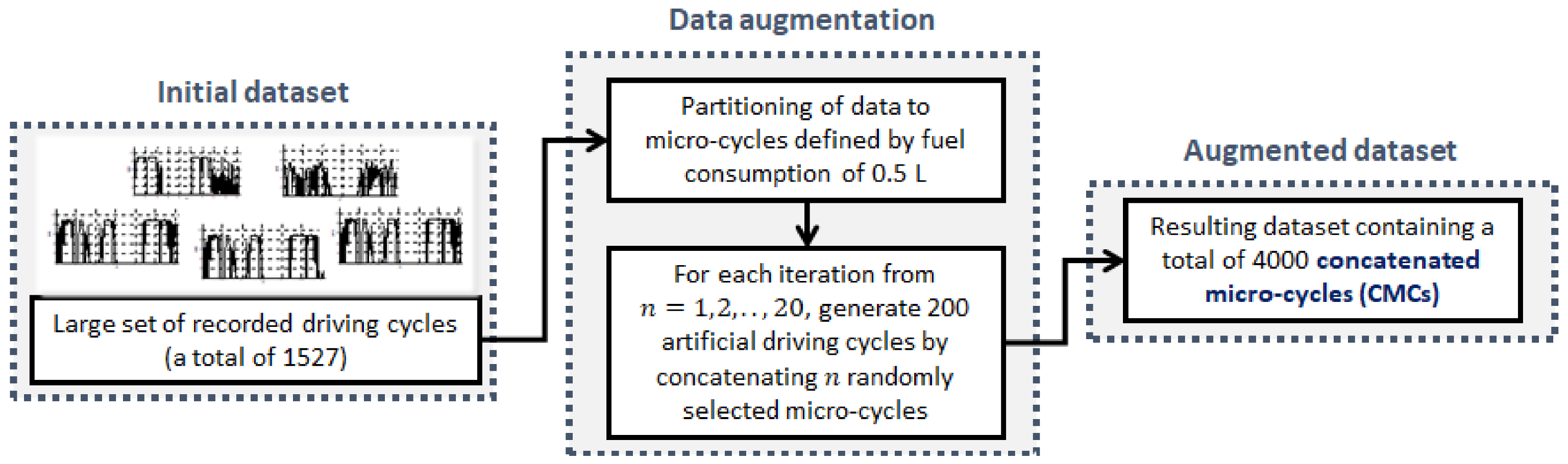
The process of driving cycle data preparation is described by the block diagram shown in Figure 6. For the purpose of well-conditioned training and testing of regression models, the recorded driving cycles are segmented into micro-cycles, where each micro-cycle is characterized by 0.5 L fuel consumption. Then, a rich set of artificial driving cycles based on combining a different number of randomly chosen micro-cycles is generated. More specifically, a total of 4000 concatenated micro-cycles (CMCs) are generated, with distance travelled covered up to 30 km, and fuel consumption from 0.5 L to 10 L. This resulted in a very diversified dataset when compared to the initial one (i.e., the one with the constant distance of approximately 5.1 km, Figure 3a). For the sake of prediction model development, the CMCs are randomly divided into three subsets aimed to be used for the training, validation, and testing of fuel consumption prediction models, with the shares of 70%, 15%, and 15% of total data, respectively. The training dataset is used to learn model, the validation dataset is used for tuning the model hyperparameters and to prevent overfitting (used only for NN parameterization; see Section 4.4), while the test dataset is aimed at an unbiased evaluation of model performance.

4.2. Nominating Initial Set of Statistical Features

A total of 91 driving cycle-related statistical features are nominated as candidates to describe a variety of driving patterns, where a detailed nomination list is presented in [34]. The statistical features are categorized into several groups related to velocity, acceleration, road slope, trip duration and length, driving characteristics, cross-correlation of velocity-acceleration-road slope, and frequency response. The following discrete time profiles are used to calculate the corresponding statistical features:

• velocity $\mathit{v}$, acceleration $\mathit{a}$, and road slope $\mathit{\theta }$,
• total power on the wheels ${\mathit{P}}_{\mathit{w}}={\mathit{F}}_{\mathit{w}}\circ \mathit{v}$ (where the operator $\circ$ denotes element-wise multiplication),
• horizontal velocity component ${\mathit{\phi }}_{\mathit{h}}=\mathit{v}\circ \cos \mathit{\theta }$,
• vertical velocity component ${\mathit{\phi }}_{\mathit{v}}=\mathit{v}\circ \sin \mathit{\theta }$,
• and power-to-mass ratio (i.e., specific power) ${\mathit{P}}_{\mathit{M}\mathit{R}}=\mathit{v}\circ \mathit{a}$,
• specific driving cycle energy per kilometre ${\mathit{E}}_{\mathit{d}\mathit{c}}={\mathit{P}}_{\mathit{w}}·\Delta T/d$ (sampling time $\Delta T$ is 1 s and $d$ is a total distance travelled),

where the total driving force ${\mathit{F}}_{\mathit{w}}$ is calculated by using a common vehicle longitudinal dynamics model given in [34].

General statistical features of discrete time profiles include minimum, maximum, mean value, standard deviation, and root mean square, while in the case of amplitude-frequency response only the mean value, standard deviation, and root mean square are used. Additional indicators are included in the case of a road slope profile frequency response, which are defined as follows. First, the frequency axis is divided into two intervals/modes, whose ranges are determined by visual inspection of the corresponding frequency response profiles (i.e., [0, 0.0025⟩ m⁻¹ for the first mode, and [0.0025, 0.005] m⁻¹ for the second mode). Then, the ratio of maximum and mean amplitude value is calculated for each of these two dominant, low-mid frequency bands.

4.3. Selection of Significant Statistical Features Based on Linear Regression Models

From the perspective of driving cycle validation, it is important to find out which features are the most influential in relation to the key, fuel consumption response variable. The relevance of each statistical feature is determined based on linear regression modelling, as described by the block diagram in Figure 7.

Firstly, a simple LR model is considered under the assumption of a linear relationship between the response variable $y_i$ and the predictor variables $x_{ij}$, and a normal distribution of response variable:

$$y_i={\beta }_0+x_{i1}{\beta }_1+\dots +x_{ij}{\beta }_j={{\displaystyle \sum }}_j{x}_{ij}{\beta }_j; i=1,2,\dots ,N; j=1,2,\dots ,M;$$

(4)

$$y_i ~ N\left({\mu }_i,{\sigma }^2\right); i=1,2,\dots ,N;$$

(5)

where ${\beta }_0,{\beta }_1,\dots ,{\beta }_j$ are the regression model parameters, ${\mu }_i$ and ${\sigma }^2$ are the response variable distribution mean value and variance, respectively, and $N$ and $M$ are the total number of observations and driving cycle-related statistical features, respectively. This model can also be written in a matrix notation as:

$$Y=X\mathsf{\beta }$$

(6)

containing the response vector $Y_{N\times 1}$, the design matrix $X_{N\times M}$, and the coefficient vector ${\mathsf{\beta }}_{M\times 1}$. The optimal regression coefficients $\widehat{\mathsf{\beta }}$ of LR model which minimise a mean squared error cost function can be found by solving the quadratic minimization problem:

$$\widehat{\mathsf{\beta }}=\underset{\beta }{\arg \min }\left(\frac{\parallel Y-X\mathsf{\beta }{\parallel }_2^2}{N}\right)={\left(X^{T}X\right)}^{-1}{X}^{T}y.$$

(7)

Secondly, the LASSO regression method is introduced, which performs feature selection through shrinking (L1 regularization) to enhance the interpretability of the given linear model and avoid overfitting (Equation (4)) [31]. The L1 regularization adds a penalty equal to the sum of absolute values of regression coefficients to the loss function defined in Equation (7). Thus, the LASSO estimate is defined by the solution to L1-constrained optimization problem:

$$\min \left(\frac{\parallel Y-X\mathsf{\beta }{\parallel }_2^2}{N}\right) \mathrm{subject} \mathrm{to} \parallel \mathbf{\beta }{\parallel }_1={\displaystyle \sum }_{j=1}^M\left|{\beta }_j\right|\le t,$$

(8)

where $t$ is the upper bound of the sum of model parameter absolute values (i.e., a degree of regularization). The optimization problem is equivalent to the parameter $\widehat{\mathsf{\beta }}$ estimation given in Lagrangian form as:

$$\widehat{\mathsf{\beta }}\left(\lambda \right)=\underset{\beta }{\arg \min }\left(\frac{\parallel Y-X\mathsf{\beta }{\parallel }_2^2}{N}+\lambda \parallel \mathbf{\beta }{\parallel }_1\right).$$

(9)

where $\lambda$ is the tuning parameter that controls the penalization strength, i.e., as $\lambda$ increases, the more regression coefficients are shrunk to zero and eliminated. If $\lambda =0$ is set, no parameters are eliminated, and the problem reduces to the least-square form (7).

The features that remain to have non-zero regression coefficient after the shrinking process are selected as important. The degree of influence of each feature with respect to chosen response variable is determined by the magnitude of resulting regression coefficient ${\widehat{\beta }}_j\left(\lambda \right)$.

The training and testing of LR and LASSO models have been conducted based on the prepared datasets containing CMCs (see Section 4.1). The calculated values of nominated statistical features are used as the predictor variables $x_{ij}$, while the recorded fuel consumption given in L/100 km is used as the response variable $y_i$. Accordingly, a total number of observations $N$ and statistical features $M$ are equal to 4000 and 91, respectively (one observation of statistical features per cycle). Note that the calculated values of each statistical feature are pre-scaled to the common range of 0 to 1, i.e., they are normalized with respect to corresponding minimum and maximum values. The optimal value of parameter $\lambda$ for LASSO model is obtained by means of 5-fold cross-validation.

4.4. Neural Network Model for Predicting Fuel Consumption for Synthetic Cycles

The feedforward NN model [35,36] is aimed at fuel consumption prediction for the purpose of synthetic driving cycles validation analyses. Although the linear models from Section 4.3 also provide fuel consumption predictions, the NN model is taken as a benchmark since it takes more complete information of driving cycle characteristics and has a significantly higher learning capacity then its linear counterparts.

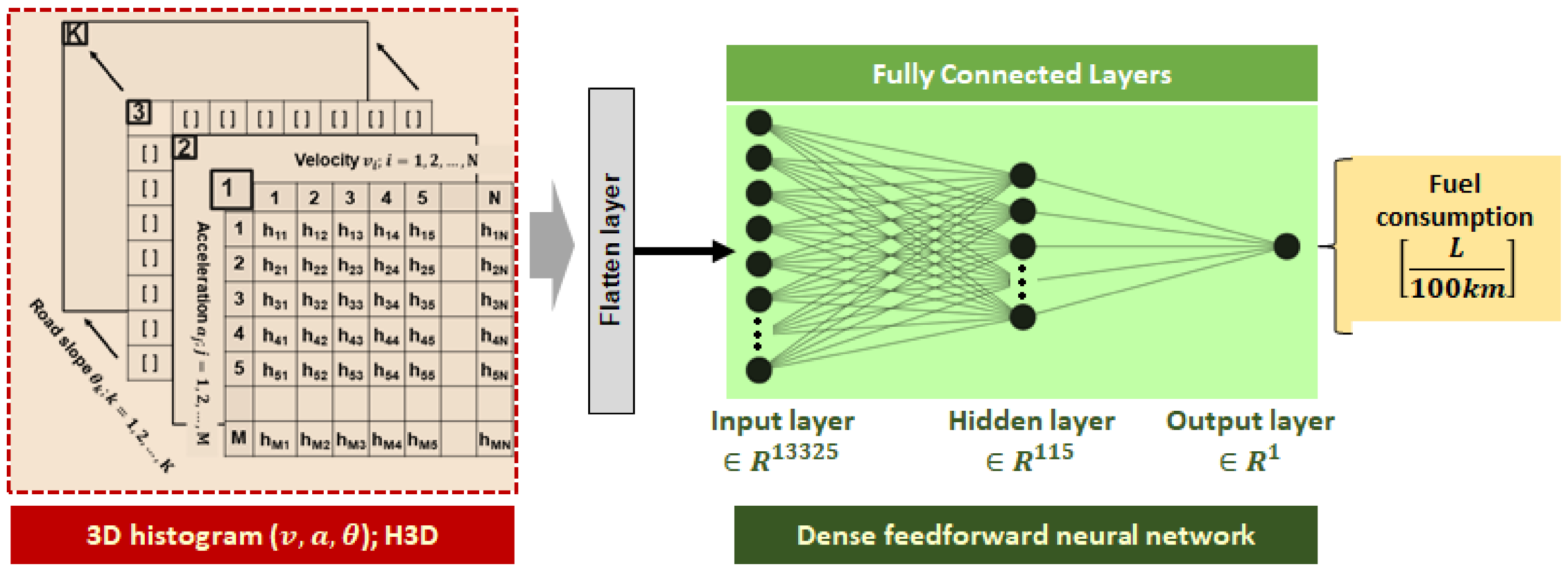
The prediction of fuel consumption is based on the (synthetic) driving cycle time series, which are conveniently transformed into a fixed-dimension 3D histogram (further labelled as H3D), whose axes correspond to discrete state values of velocity, acceleration, and road slope. The H3D serves as a static input to the NN, as shown in Figure 8. The NN architecture has been selected according to the generalization prediction error criterion, by iteratively inspecting different numbers of hidden layers and related neurons [35,37].

For the sake of NN model development, the CMCs are used (see Section 4.1 and Figure 6). The NN model is implemented within the Python environment by using Keras module [38] with Tensorflow as backend [39] and in-built Adaptive Moment Estimation (ADAM) training algorithm [37]. The batch size and the number of epochs for NN training are set to 16 and 100, respectively. The loss function to be minimized is chosen as a mean square error (MSE) of fuel consumption. The fuel consumption prediction performance is examined in Section 4.5.

4.5. Performance Analysis of Regression Models

The performance of fuel consumption prediction for LR, LASSO, and NN models, established in Section 4.3 and Section 4.4, has been examined by using the CMC test dataset (see Section 4.1). The indicators considered for evaluation of models include R² score, mean value ${\mu }_{res}$, and standard deviation ${\sigma }_{res}$ of model prediction residuals/errors. The R² indicator represents the proportion of variance in response variable which can be explained by the predictor variables. The value R² = 1 corresponds to the ideal fit, while R² = 0 means no correlation, i.e., it corresponds to the case when the model output is constant and equal to the mean value of recorded fuel consumptions.

The calculated values of the aforementioned indicators are shown in

Table 1. Performance indicators calculated for different regression models aimed at predicting fuel consumption (test dataset used).

Regression Model	${\mathit{\mu }}_{\mathit{r}\mathit{e}\mathit{s}} [\mathbf{L}/100 \mathbf{km}]$	${\mathit{\sigma }}_{\mathit{r}\mathit{e}\mathit{s}} [\mathbf{L}/100 \mathbf{km}]$	R2 [-]
LR	0.24	2.59	0.935
LASSO	0.24	2.51	0.939
NN	0.12	2.47	0.942

. The corresponding plot of predicted vs. real/recorded fuel consumption and respective probability distributions of prediction errors/residuals are shown in Figure 9. These results show that all models have similar error distribution and performance. The NN model is characterised by the highest R² of 0.942 and lowest ${\sigma }_{res}$ of 2.47 L/100 km, thus representing the ultimate prediction accuracy. Although being significantly simpler, both LR and LASSO models follow the NN model very closely, with R² equal to 0.935 and 0.939, respectively, and ${\sigma }_{res}$ being around 5% larger. It should also be noted that the predictions are well balanced, i.e., the mean error ${\mu }_{res}$ is close to zero.

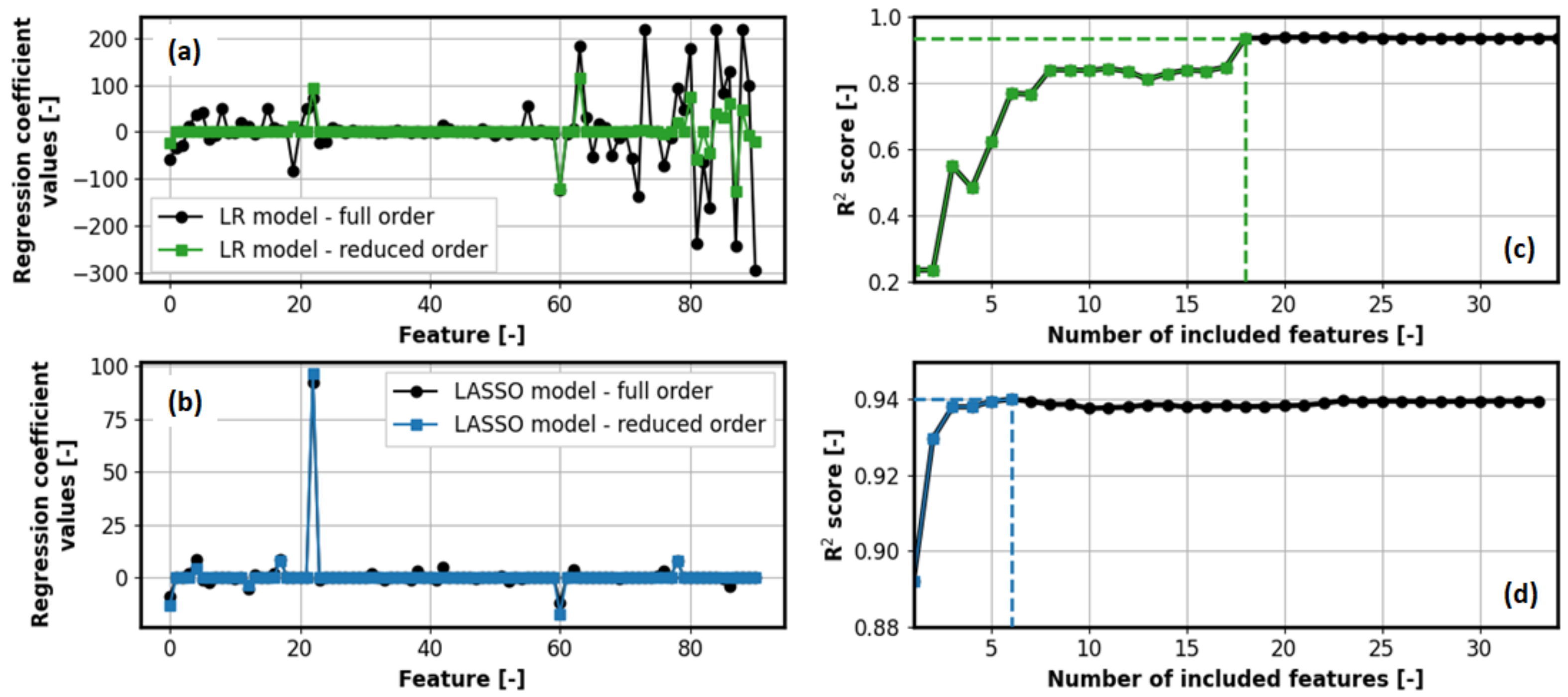
The results further show that LASSO is capable of reducing the initial set of 91 features to 33 ones (i.e., a total of 58 regression coefficients $\widehat{\beta }$ are shrunk to zero). This is illustrated in Figure 10a,b, which show the final values of the regression coefficients ${\widehat{\beta }}_j$ for each statistical feature, obtained for initial training of LR and LASSO models, respectively (curves marked in black). Moreover, in the case of counting the number of features for which the condition $\left|{\widehat{\beta }}_j\right|\le 1$ is met, the number of relevant features decreases from 33 to 21 for LASSO model (−76.9% w.r.t. initially nominated set of statistical features), and from 91 to 77 for LR model (−15.4%).

To investigate whether a further reduction in the number of features would be feasible, a sensitivity analysis of the prediction accuracy of the LR and LASSO models depending on the number of input features is performed. First, the features are sorted by relevance (i.e., ${\widehat{\beta }}_j$ value) in descending order. Next, for each subset $P_s$ including $s=1,2,\dots S$ sorted features (where S is equal to 33 and 91 for LASSO and LR model, respectively), the new models are trained, and their prediction accuracies are examined by calculating R² score on test dataset. Finally, it is checked which of the models result in a prediction accuracy close to the original model (cf. Table 1), while containing a low number of features. The obtained results indicate that in the case of LR model the first 18 features are sufficient for a given prediction task (see Figure 10c and also green plot in Figure 10a), while the first six features are sufficient for LASSO model (see Figure 10d and also blue plot in Figure 10a). Since LASSO model results in better performance and less features than LR model (R² value of 0.940 vs. 0.937 for the case of 6 vs. 18 features), it is adopted as a referent model for further analyses. The main reason for choosing LASSO instead of NN model is because it uses a limited set of features rather than the complete driving cycle information as input, and it also performs automatic feature selection through L1 regularization (see Section 4.3). Therefore, the values of the regression coefficients ${\widehat{\beta }}_j$ for the corresponding subset of six most significant features (

Table 2. Finally adopted subset of most significant features of Lasso regression model, including the corresponding regression coefficient values ${\widehat{\beta }}_j$ and minimum/maximum feature values (calculated before applying normalization).

No.	Feature	Min/Max Values	Unit	Regression Coefficient Value *
1.	Mean specific driving energy per kilometre travelled $\left({\overline{E}}_{dc}^{+}={\displaystyle \sum }_{k=1}^N{E}_{dc,k}; \forall E_{dc,k}>0\right)$	1.23/14.31	MJ/km	98.11
2.	Standard deviation of vertical velocity component	0.02/1.82	km/h	−16.35
3.	Mean velocity	0.05/41.69	km/h	−16.34
4.	Root mean square of amplitude of road slope frequency response	0.39/5.23	-	7.93
5.	Number of vehicle stops per kilometre	0/8.37	km−1	7.17
6.	Mean positive acceleration	0.22/1.12	m/s2	3.91
7.	Intercept			33.52

* Given regression coefficient values are obtained for a case involving min-max normalization of input features.

) are utilized for further validation of synthetic driving cycles. Note that the small excess or shortfall in resulting R² values for the case of reduced order models when compared to full order models (cf. the above R² values with those given in Table 1) are the result of better or worse generalization on unseen/testing data.

5. Validation of Synthetic Driving Cycles

First, a combined driving cycle is introduced (further abbreviated as Comb), which is obtained by concatenating all individual recorded driving cycles. Thus, the statistical feature values calculated for Comb cycle represent the average values of those obtained for individual driving cycles. The synthetic driving cycles whose statistical features are closer to the mean values of those related to the recorded Comb cycle are considered to be more representative. Next, a novel lumped performance indicator is derived based on a subset of six significant features obtained through LASSO regression-based feature selection method (Table 2), and it is compared with the previously considered Euclidean distance of statistical feature deviations from Comb values. The aim is to consolidate the overall set of statistical indicators into a single metric that determines how closely a synthetic driving cycles follows the expected/mean values of the Comb recorded driving cycles, thus enabling unambiguous validation of numerous generated synthetic driving cycles. Finally, a few most representative driving cycles are selected by using the derived lumped performance indicators and are thoroughly analysed with respect to statistical feature values.

5.1. Lumped Performance Indicators

In the recent study [34], various feature-related lumped performance indicators have been derived and compared with respect to fuel consumption deviation (FCD) to reveal the most suitable one for validation. Note that the FCD is defined as the absolute deviation of synthetic driving cycle fuel consumption $V_{f,syn,i}$ (predicted by using the NN model proposed in Section 4) with respect to fuel consumption calculated for Comb cycle ${\overline{V}}_{f,Comb}$:

$${\mathrm{FCD}}_i=\left|V_{f,syn,i}-{\overline{V}}_{f,Comb}\right|,$$

(10)

where $i$ represents ith synthetic driving cycle (out of a total of 3000 ones generated).

The results of the correlation analysis of given performance indicators with respect to FCD have shown that the Euclidean distance (ED) turns out to be the most suitable indicator for validation of driving cycles [34], and it is defined as:

$${\mathrm{ED}}_i=\sqrt{{\displaystyle \sum }_j^M{\left({\overline{X}}_{Comb,j}-X_{syn,ij}\right)}^2},$$

(11)

where ${\overline{X}}_{Comb,j}$ represents value of jth statistical feature for Comb cycle, $X_{syn,ij}$ represents value of the same (jth) statistical feature for ith synthetic driving cycle, and $M$ is the number of all considered statistical features (equal to 91, herein).

Furthermore, a novel performance indicator labelled as Regression Index (further abbreviated as RI) is proposed, which is derived from the reduced-order LASSO regression model coefficients ${\widehat{\beta }}_j$(Table 2), as:

$${\mathrm{RI}}_i=\left|V_{f,LASSO,i}-{\overline{V}}_{f,LASSO,Comb}\right|\equiv \left|{\displaystyle \sum }_j^M{\widehat{\beta }}_j\left(X_{syn,ij}-{\overline{X}}_{Comb,j}\right)\right|,$$

(12)

It is of interest to determine if the newly proposed and easier-to-calculate performance indicator is more accurate/representative than the ED indicator, which is done by conducting a correlation analysis of RI with regard to FCD (see Section 5.2.).

5.2. Correlation Analysis of Lumped Performance Indicators with Respect to Fuel Consumption Deviation

The performance indicators (including the FCD) defined in Section 5.1 are calculated for each synthetic driving cycle. For the purpose of correlation analysis, the Pearson correlation coefficient $\rho$ (function corrcoef from numpy module in Python) has been utilized as a measure of how two variables are related to each other.

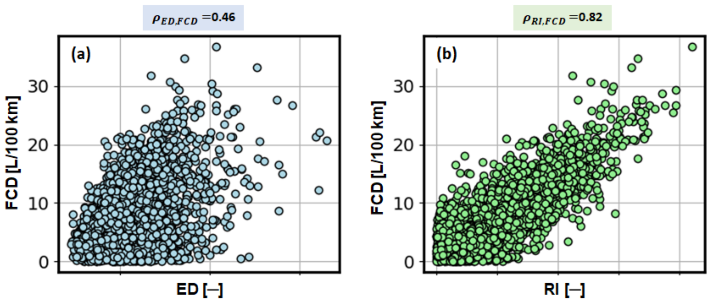
The dependence of ED and RI performance indicators with respect to FCD are shown in Figure 11. The corresponding correlation coefficients are equal to 0.82 for RI and 0.46 for ED, which clearly reveals dominance of RI over ED. Hence, the RI is adopted as the final performance indicator for validation of synthetic driving cycles (see Section 5.3.). Note that the main advantage of RI over FCD is that, once the relevant driving cycle features are selected (Table 2), there is no need to use fuel consumption information for validation of synthetic driving cycles.

5.3. Selection of Representative Driving Cycles

Let $\mathsf{\Psi }=\left\{{\mathbf{\psi }}_1,{\mathbf{\psi }}_2,\dots ,{\mathbf{\psi }}_N\right\}$ be the overall set of synthetic driving cycles, where N represents their total number (equal to 3000, herein), and ${\mathbf{\psi }}_i=\left[{\mathit{v}}_i {\mathit{a}}_i {\mathit{\theta }}_i \dot{{\mathit{\theta }}_i}\right];i=1,2,\dots ,N$. Note that each ${\mathbf{\psi }}_i$ includes calculated value of performance indicators ${\mathrm{RI}}_i$ and ${\mathrm{ED}}_i$. The most representative driving cycle ${\mathbf{\psi }}^{*}$ is found according to the criterion of the minimum RI (or ED) as:

$${\mathbf{\psi }}_{\mathrm{RI}}^{*}=\underset{\mathsf{\Psi }}{\arg \min }\left(\mathrm{RI}\left(\mathbf{\psi }\right)\right) \mathrm{or} {\mathbf{\psi }}_{\mathrm{ED}}^{*}=\underset{\mathsf{\Psi }}{\arg \min }\left(\mathrm{ED}\left(\mathbf{\psi }\right)\right).$$

(13)

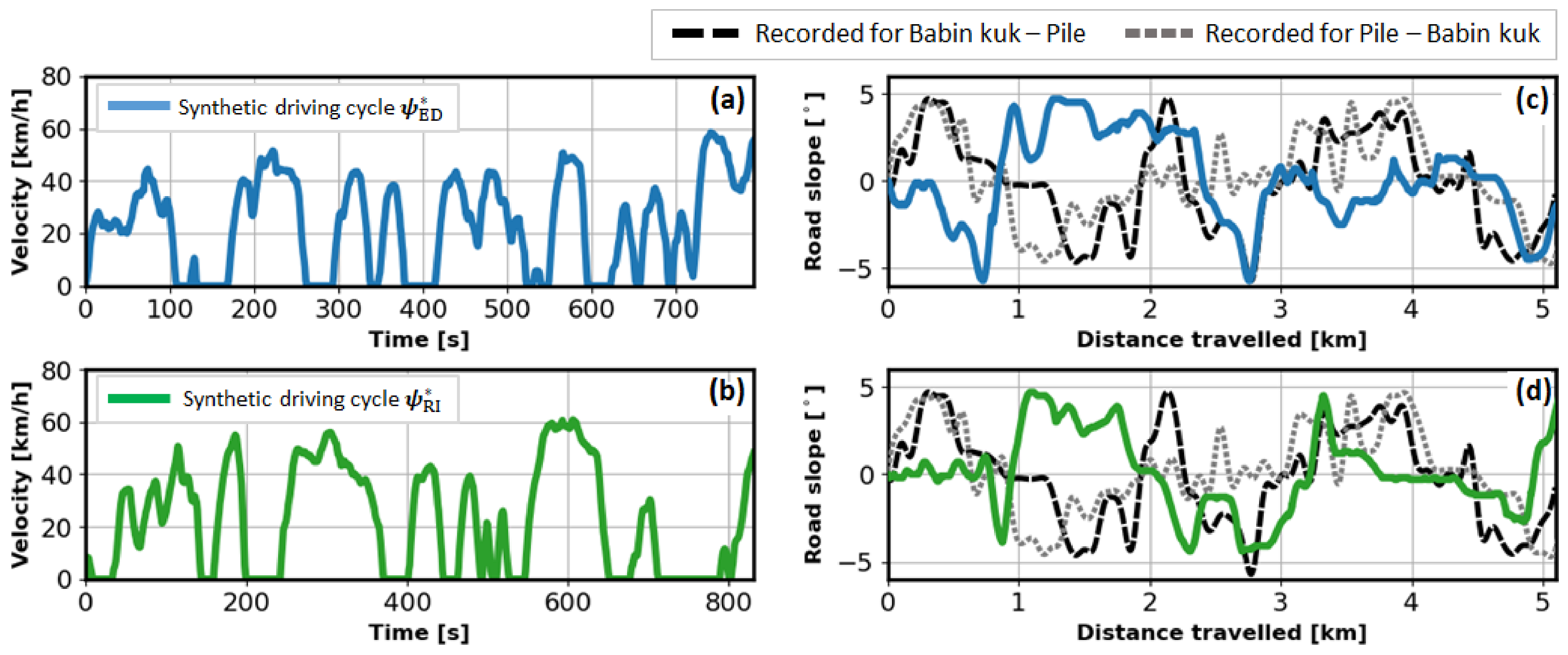
The most representative synthetic driving cycles ${\mathbf{\psi }}_{\mathrm{RI}}^{*}$ and ${\mathbf{\psi }}_{\mathrm{ED}}^{*}$, selected according to the criteria defined in Equation (13), are further compared in terms of their statistical characteristics. The resulting velocity vs. time profiles of the selected driving cycles, along with the corresponding road slope vs. distance travelled profiles are shown in Figure 12 (including the recorded profiles in the latter case, for both driving directions; cf. Figure 4). Note that differences in synthetic road slope profiles when compared to the recorded profiles are simply the result of stochasticity of synthetic cycles generation process (see Section 3). Nevertheless, they retain statistical properties of the recorded road slope profiles (e.g., amplitude and frequency in Figure 12c,d), including the cross-correlation with vehicle velocity and acceleration profiles.

Finally, a comparative analysis of statistical characteristics of extracted, most representative driving cycles according to the ED and RI criteria is performed. The calculated values of statistical features of driving cycles ${\mathbf{\psi }}_{RI}^{*}$ and ${\mathbf{\psi }}_{ED}^{*}$ are given in

Table 3. Values of selected statistical features for combined recorded cycle (Comb) and most representative synthetic driving cycles selected according to RI and ED criteria.

No.	Statistical Feature	Unit	Comb	Most Representative Driving Cycle
				${\mathit{\psi }}_{\mathbf{ED}}^{*}$	${\mathit{\psi }}_{\mathbf{RI}}^{*}$
1.	Mean velocity	km/h	23.03	23.25 (+1.0%) 1	22.18 (−3.7%)
2.	Mean positive acceleration	m/s2	0.45	0.48 (+5.6%)	0.47 (+3.6%)
3.	Number of stops per kilometre	km−1	1.87	2.15 (+15.0%)	1.95 (+4.5%)
4.	Mean specific driving energy per kilometre travelled	MJ/km	4.32	4.45 (+3.2%)	4.40 (+2.0%)
5.	Standard deviation of vertical velocity component	km/h	1.34	1.32 (−1.5%)	1.16 (−13.5%)
6.	Root mean square of amplitude of road slope frequency response	-	1.33	1.25 (−6.0%)	1.08 (−19.1%)
7.	Standard deviation of road slope	°	2.59	2.41 (−6.6%)	2.44 (−5.5%)
8.	Standard deviation of the total power on the wheels	kW	67.46	65.55 (−2.8%)	64.33 (−4.6%)
9.	Standard deviation of power-to-mass ratio	W/kg	3.61	3.64 (+0.8%)	3.47 (−3.9%)
10.	Fuel consumption	L/100 km	39.84	42.87 (+7.6%)	41.05 (+3.0%)

¹ Values in parentheses represent relative differences of statistical features from the ones related to Comb driving cycle.

, and they are compared to the corresponding values of recorded Comb cycle. Since the initial set contains a large number of statistical features (a total of 91), the comparison is made only for a reduced subset of 10 features listed (Table 3). These features include the six most significant ones from Table 2 and additional ones related to fuel consumption and standard deviations of road slope, total wheel power and power-to-mass ratio. The results shown in Table 3 indicate roughly equal matching of considered statistical features for ED and RI criteria (majority of 10 selected features are within ±10% difference from those of Comb). However, the advantage of RI over ED is in the lower deviation in fuel consumption feature (+3.0% for ${\mathbf{\psi }}_{\mathrm{RI}}^{*}$ vs. +7.6% for ${\mathbf{\psi }}_{\mathrm{ED}}^{*}$), and similarly the feature of mean specific driving energy (MSDE) per kilometre travelled (+2.0% for ${\mathbf{\psi }}_{\mathrm{RI}}^{*}$ vs. +3.2% for ${\mathbf{\psi }}_{\mathrm{ED}}^{*}$). The former is because the RI directly reflects the fuel consumption (see Equation (12)), while the latter is because the MSDE is the most significant predictor variable selected by the LASSO method (see Table 2) and is closely related to fuel consumption. Note that it is generally possible to apply multi-criteria validation based on various performance indicators (e.g., ED, RI and FCD) to find a synthetic driving cycle that represents a trade-off between each performance indicator considered [34].

6. Discussion

The presented study has demonstrated that by applying the proposed multidimensional driving cycle synthesis and validation method it is possible to synthesise representative driving cycles in a straightforward and computationally efficient way. The representativeness is reflected through considering a rich set of statistical features extracted from real driving patterns. The synthesised driving cycles can be used in various simulation and also dynamometer test studies, where a large set of recorded cycles should be replaced by a single or a couple of representative cycles (e.g., for vehicle design studies, certification purposes, and similar), or where there is a need to generate a large number of synthetic cycles (e.g., for sensitivity analyses).

Moreover, the presented method extracts the most significant driving cycle features and a corresponding linear regression model that predicts the fuel/energy consumption. As such, it can be used to predict fuel consumption and similarly pollutant and greenhouse gas emissions based on several features (e.g., mean velocity, mean positive acceleration, road slope standard deviation, number of vehicle stops and similar), which could be obtained based on standard, low-resolution vehicle tracking data (typically sampled every 20–40 s). This allows for predicting energy consumption based on readily available data in a very computationally efficient way (i.e., without using micro-simulations based on high-resolution driving cycles), in order to support various transport system planning and optimisation studies.

These simple regression models can also be used in a variety of electromobility applications, such as city bus transport electrification planning. For example, transport officers can employ a virtual macro-simulation framework, which, based on available route timetables and historical measurement data, estimates the buses’ arrival and dwelling times at end stations and predict the energy consumed for each trip. The macro-simulation framework can be used for various transport and energy planning studies, e.g., finding of optimal charging infrastructure configuration in terms of charging station allocation, number of chargers, buses battery capacity, etc. [40]. Moreover, the results of using such a planning tool can be of significant benefit to policy makers in terms of providing recommendations for improvements in public transport service and cost competitiveness of electrified fleet. Other applications of developed regression models are related to vehicle routing problems (VRP) [41], which due to their high computational complexity require approximate energy consumption models that are executed swiftly.

The main foreseen limitation of the presented regression-based energy consumption prediction, when compared to prediction based on physical model-based microsimulations, is in potential extrapolation issues. Namely, it is possible that the augmented dataset used to train the regression model do not cover the entire statistical feature space, which may lead to a situation where the model encounters unseen data and give inaccurate fuel consumption predictions. This includes the situations in which the selected features do not reflect some relevant vehicle operating parameters, such as external temperature, which affects the air conditioning (A/C), and thus overall energy consumption.

To demonstrate the discussed application opportunities, as well as overcome limitations, a broader research study is needed based on a comprehensive set of transport data, which is a subject of current and future work. Moreover, additional effort can be invested in the application and assessment of other feature selection methods, such as filter-based, wrapper-based, and other embedded methods.

7. Conclusions

The paper has presented a method for the synthesis of multidimensional driving cycles based on the Markov chain model, which, in addition to vehicle velocity and acceleration states, also accounts for road slope and its time derivative. Special emphasis was on validation of synthesized driving cycles based on a rich set of statistical features, including the indicators related to vehicle velocity, vehicle acceleration, road slope, driving characteristics, cross-correlation of velocity-acceleration-road slope, and respective frequency responses. To improve computational efficiency and reduce memory demand, the eight-dimensional transition probability matrix (TPM) was implemented in a sparse form based on a dictionary of keys. Numerous synthetic driving cycles were generated by sampling from TPM, and the values of selected statistical features were calculated for each of them. An accurate neural network (NN) model was developed for predicting the fuel consumption based on synthetic driving cycles. A subset of most significant statistical features was established by using the least absolute shrinkage and selection operator (LASSO) method and used for determining a unique performance indicator for unambiguous driving cycle validation.

The LASSO-based linear regression analysis has pointed out that an exceptional prediction accuracy (i.e., competitive to a more complex neural network) can be accomplished by using a reduced set of only six (out of 91) most significant driving cycle statistical features as inputs to the regression model. The most significant features selected are mean velocity, mean positive acceleration, number of stops per kilometre, standard deviation of vertical velocity component, root mean square of amplitude of road slope frequency response, and mean specific driving energy per kilometre travelled. The correlation analysis in relation to fuel consumption deviation (FCD) with respect to concatenated recorded driving cycle has pointed out that the newly proposed LASSO regression indicator (RI) correlates better with the FCD than the previously proposed Euclidean distance (ED) indicator (the correlation index is 0.82 vs. 0.46). Additionally, it has been shown that, based on RI, a single most representative synthetic driving cycle can be selected in a straightforward way. Finally, the dominance of RI over ED in terms of synthesizing a representative driving cycle in terms of fuel consumption has been demonstrated.