Smart Steaming: A New Flexible Paradigm for Synchromodal Logistics

Abstract

Slow steaming, i.e., the possibility to ship vessels at a significantly slower speed than their nominal one, has been widely studied and implemented to improve the sustainability of long-haul supply chains. However, to create an efficient symbiosis with the paradigm of synchromodality, an evolution of slow steaming called smart steaming is introduced. Smart steaming is about defining a medium speed execution of shipping movements and the real-time adjustment (acceleration and deceleration) of traveling speeds to pursue the entire logistic system’s overall efficiency and sustainability. For instance, congestion in handling facilities (intermodal hubs, ports, and rail stations) is often caused by the common wish to arrive as soon as possible. Therefore, smart steaming would help avoid bottlenecks, allowing better synchronization and decreasing waiting time at ports or handling facilities. This work aims to discuss the strict relationships between smart steaming and synchromodality and show the potential impact of moving from slow steaming to smart steaming in terms of sustainability and efficiency. Moreover, we will propose an analysis considering the pros, cons, opportunities, and risks of managing operations under this new policy.

1. Introduction

In Europe, it is estimated that the transport sector produces one-quarter of the total greenhouse gas emissions, also contributing to worsening the air quality in cities (https://ec.europa.eu/clima/policies/transport_en, accessed on 7 April 2021). Moreover, the transport industry has not been able to reduce emissions fast enough compared to other sectors like energy and agriculture, being the only sector currently keeping a level of emissions higher than that registered during the ’90s. More precisely, heavy-duty road vehicles, like trucks and buses, are responsible for about one-quarter of all road transportation emissions, producing approximately 5% of the total EU emissions (https://ec.europa.eu/clima/policies/transport/vehicles_en, accessed on 7 April 2021). Instead, the maritime shipping sector is responsible for 13% of the overall greenhouse gas emissions in the European Union and 2.5% globally (https://ec.europa.eu/clima/policies/transport/shipping_en, accessed on 7 April 2021). From a global perspective, the maritime transport system carries over 90% of the world’s trade volume. The largest naval carbon emitters and ocean freight contribute approximately 5% of the global carbon emissions [1].

To reduce ship emissions, the International Maritime Organization suggested three approaches: the enlargement of vessel size, the utilization of new technologies, and the reduction of voyage speed [2]. Concerning this last point, it is well known that fuel consumption is not proportional to the vehicle’s speed and that slower speeds allow for fuel saving. For this reason, slow steaming (i.e., the possibility to ship vessels at a significantly slower speed than their nominal one) became common practice around 2008 along the Europe–Far East trade route and also gained in importance on other trade routes in the following years, as a response of shipping lines to the fast-rising bunker costs and the surplus of capacity created by the concurrent economic crisis [3]. Slow steaming has also been integrated within the recent logistics paradigm called synchromodality. It consists of providing efficient, reliable, flexible, and sustainable services through the coordination of stakeholders and the synchronization of operations within a complex supply network using modern technology solutions [4]. The two paradigms can strongly reduce operational costs and environmental externalities, making their combination an attractive solution, especially for long-haul shipments [5].

However, slow steaming is not flexible enough to exploit the full potential deriving by adopting synchromodal logistics. Therefore, an evolution of such a paradigm called smart steaming is presented and deeply discussed in this paper. Smart steaming is the real-time synchronization of the operations by considering the possibility of slowing down or speeding up vehicles, according to real-time information and a more comprehensive view of the network with a multi-stakeholder approach. For this reason, smart steaming better integrates with synchromodality. Moreover, it represents a new strategy to achieve a sophisticated planning (one of the main critical success factors for the implementation of synchromodality [6]), as the efficient re-planning of shipments, routes, and cargos with high operational flexibility brings significant benefits [7].

This work provides the following scientific contributions: We present the smart steaming paradigm for the first time in the literature by discussing its peculiar characteristics and related strategies and operations. The concept has appeared before only within a European project called SYNCHRO-NET, but it was never formalized to the best of our knowledge. First, we discuss smart steaming’s foundation by analyzing and linking together four established practices: slow steaming, synchromodality, fuel consumption models, and speed optimization problems. Within the synchromodal logistics context, we discuss the paradigms’ limitations to justify introducing a new one. Second, a complete overview of the smart steaming paradigm’s features is presented to propose a more efficient and sustainable approach in managing long-haul transportation and logistics operations. Third, we perform an analysis of the impact and the difficulties of implementing smart steaming in an existing logistics network. Finally, we present some optimization paradigms to deal with uncertainty and the different decision problems arising at the various planning levels while adopting the smart steaming strategy.

The paper is structured as follows. In Section 2, we discuss the four foundation blocks of smart steaming, gathering the related scientific literature. In Section 3, we present the smart steaming paradigm and its features. In Section 4, we discuss smart steaming’s real-life implementation considering possible issues and benefits. In Section 5, we use the previous analysis results to derive important insights into tackling optimization problems in this context. In Section 6, we summarize the main results of this work and propose future research lines.

2. Background and Established Practices: Towards a Smart Steaming Paradigm

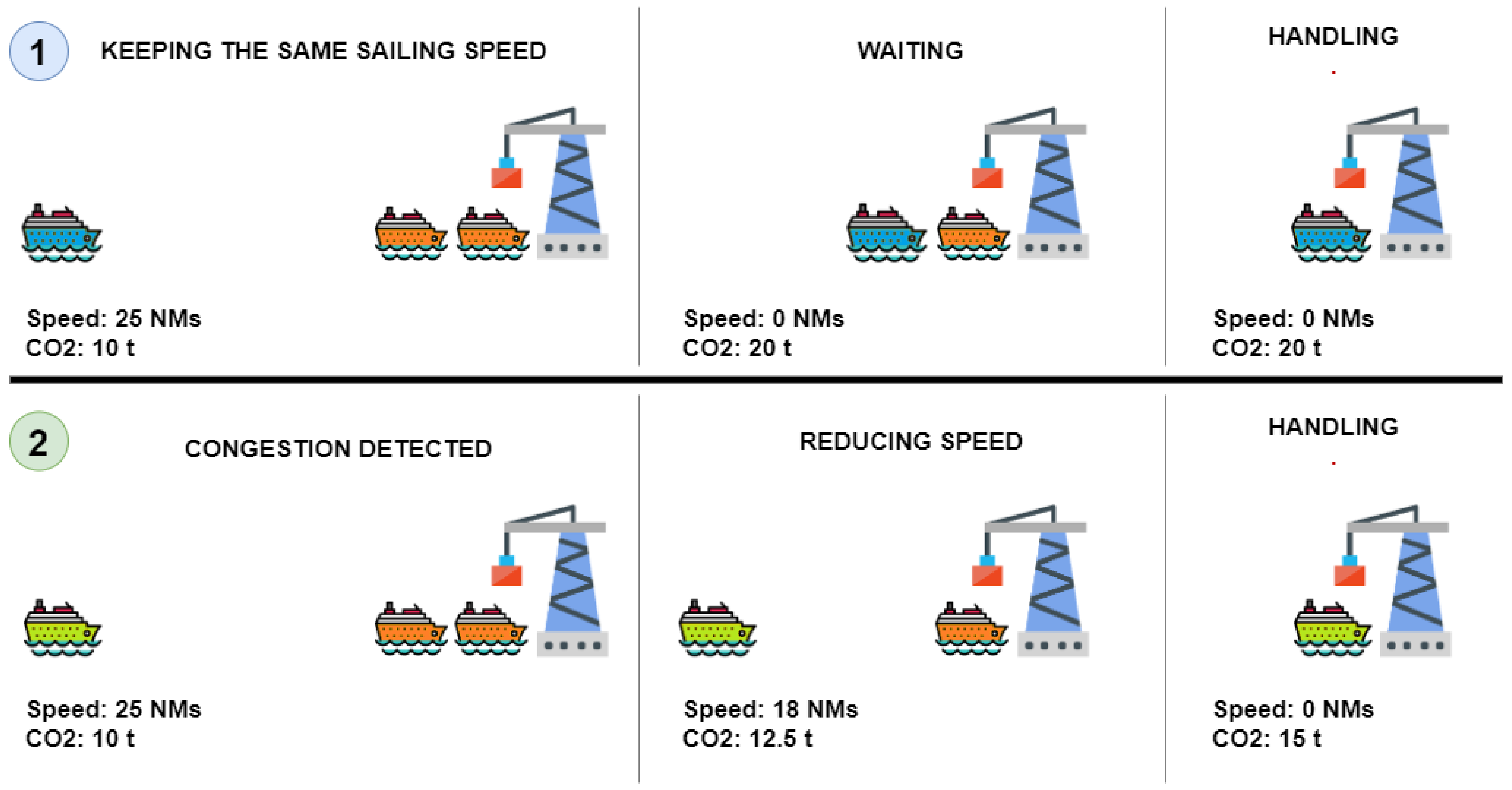
This section discusses four critical topics for understanding logistics’ current status and derives a reasonable justification of the smart steaming paradigm’s need. First, we overview the slow steaming paradigm that can be considered as the predecessor to the smart steaming’s paradigm (Section 2.1). Second, we focus on synchromodality that will be the perfect context in which smart steaming can be implemented (Section 2.2). Third, we discuss the fuel consumption models to get insights into the main factors for emissions of the various transportation modes (Section 2.3). Finally, we discuss the current status of speed optimization problems and their limitations concerning what will be considered in smart steaming (Section 2.4).

2.1. Slow Steaming

Slow steaming has been adopted as a strategy to solve problems related to the oversupply of shipping capacity, the increase of fuel price, and the sustainability of transportation operations [8]. Transporting containers by ships with the slow steaming strategy has already proved its potential to decrease emissions, reduce fuel consumption, improve fleet capacity utilization, and provide more reliable schedules [9,10,11]. However, the advantages provided by slow steaming are strictly related to many factors that can be grouped into three categories: market-, fleet-, and route-related factors.

From an economic point of view, companies can benefit by slowing down vessels only if there are certain market conditions as low freight rates, high fuel prices, overcapacity, and low demand [12,13]. Sometimes, instead, adopting slow steaming may become inconvenient as its benefits may not be enough to cope with the fall of fuel prices and the increase of other costs (e.g., inventory) [14]. For these reasons, it is essential to find policies and strategies that reduce emissions while providing good profits. In general, decision-makers tend to prefer more profitable solutions instead of the greener ones [15], but adopting some strict environmental policies can mitigate the market-related factors [16].

Route-related factors are strictly related to the characteristics of specific areas, regions, or nations. For instance, slow steaming is considered one feasible strategy to comply with emission regulations in certain areas, but high speeds with higher emissions are preferred elsewhere [17,18]. However, environmental regulations become stricter and stricter every year, thus requiring to study of the combination of slow steaming with other strategies (e.g., biofuels, re-routing, timetable adjustments, and larger multifunctional vessels) to mitigate the adverse effects on operational costs [19]. Other aspects regarding routes are related to the length of the journey, making slow steaming more effective for long-haul transportation (e.g., oceanic routes) compared to the short-haul one, mainly due to the higher competitiveness with other transportation modes [20]. Besides the route length, the status of the ports’ operations might require to increase or reduce the optimal speed of the vehicles [21].

Regarding the fleet, adopting slow steaming reduces the number of possible travels for the vehicles over a time horizon (e.g., per year), diminishing the overall capacity. Reducing the available services can lead to negative consequences on revenues, but these can possibly be compensated by the savings on operational and fuel costs [22]. Therefore, adopting slow steaming may require more vehicles and larger ones to maintain the same service quality and satisfy all the demand. Moreover, implementing a long-term strategic speed reduction policy will require modifying the ships’ design (e.g., hull shapes and engine characteristics) [23]. Considering these aspects to adopt new service design strategies is crucial to plan a heterogeneous and competitive fleet that combines fast and direct services with cheaper but slower ones [24].

Various analytical tools considering some or all of the above-described factors have been implemented to study the slow steaming impact. For instance, Mallidis et al. [25] developed an analytical modeling methodology for evaluating the effects of slow steaming on travel and logistics costs for various stakeholders. They used this approach in a real case study to understand how a carrier and a shipper can divide the savings provided using the slow steaming strategy. Another work evaluating the effect on costs can be found in Xiong et al. [26], which presented a two-echelon inventory management model considering the impact on the costs of changing the speed of inland river vessels. Focusing more on the sustainable aspect, Le et al. [27] designed a tool based on an artificial neural network, trained with actual operational data, to demonstrate the crucial role of slow steaming in reducing fuel consumption and emissions. Companies that need to find the right slow steaming level can use this tool to reach their energy efficiency goals. Last, a recent initiative, the so-called virtual arrival, shows that good coordination of vessels’ arrival times can decrease the planned costs and emission while mitigating congestion at ports [28]. Therefore, calculating appropriate buffer times (e.g., using historical data of ports delay) on all routes to mitigate uncertainty with the flexibility to speed up can improve the service quality and reliability [29]. Therefore, this highlights how coordination and flexible speeds allow for better results than the vessels’ pure slowing down.

To summarize, slow steaming can be a good practice to reduce costs and emissions, but some market, fleet, and route conditions may make it unprofitable. Moreover, the literature mainly focuses on the speed optimization of a single ship or different vessels traveling on a single route. There is a lack of a broader view considering supply chain networks using more modes of transportation with vehicles adopting dynamic speeds to avoid disruptions (e.g., port congestion, traffics, and accidents), reduce emissions and increase revenues, and improve the quality of the services. Moreover, an effort on the various planning levels is required. From a strategic point of view, investments to expand and upgrade the technological fleet-level are needed. At the operational level, methods to evaluate the vehicles’ ideal speeds in real-time are required. For these reasons, in this work, we propose the smart steaming paradigm as a more robust and flexible evolution of slow steaming into the context of the most recent synchromodal logistics contexts, taking into account fuel consumption models of the various transportation modes.

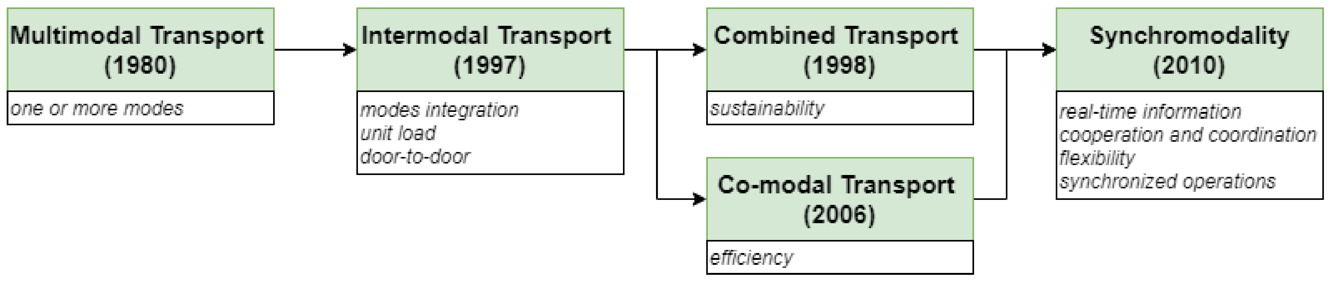
2.2. Synchromodality

It is essential here to present a brief overview of synchromodality to understand how the slow steaming paradigm must evolve to fit this context. For an exhaustive treatment on synchromodal logistics, the reader is referred to Giusti et al. [4].

The term synchromodality was recently coined to adapt the already existing multimodality, intermodality, combined transport, and co-modal transport terms to the most modern and complex logistics contexts. An evolution scheme of all such paradigms with their characteristics, included synchromodality, is shown in Figure 1.

Synchromodality inherits several features like the utilization of different modes of transportation, the integration between transportation modes using the same unit load, and the efficiency and the sustainability of the operations [30]. Ideally, these features are used in synchromodality to offer door-to-door container shipping services. Shipments are performed by following origin, destination, and due date constraints of the customers, but with the freedom of choosing who provides the transportation services, which paths are used, and how the transshipment operations are performed. This freedom gives more flexibility to obtain an overall optimized plan. Besides the features inherited from preexisting paradigms, synchromodality has at least four peculiarities adopted to provide even better results:

• real-time information management,
• service flexibility,
• stakeholders cooperation and coordination, and
• synchronization of the operations.

In a network managed under the synchromodality paradigm, all the stakeholders must access all the relevant information in real-time. This allows monitoring the operations’ status to coordinate all the activities and adopt real-time countermeasures against unexpected disruptions. For instance, the so-called real-time switching consists of changing the container routing to respond to events like service delays or cancellations [31]. To make the best use of real-time information, both customers and whoever is performing the logistics operations must ensure a certain degree of flexibility for adopting re-planning solutions. For instance, customers should adopt mode-free booking, the so-called a-modal booking, that offers the flexibility to logistics service providers (LSPs) to plan the shipments by combining multiple orders and routing them with various transportation modes [32]. Instead, the collaborators contracted by LSPs should be more flexible in performing their operations, allowing re-planning instead of having strictly fixed plans. On the other hand, sharing information in real-time and adopting a more flexible approach requires stronger cooperation. This means that, under synchromodality, assuming only the classical vertical cooperation (i.e., among stakeholders operating at different levels) is not sufficient. Furthermore, horizontal cooperation, i.e., among stakeholders doing similar activities (e.g., transportation services in different modes), is required [33]. A particular LSP must operate as an orchestrator, which contracts other stakeholders (e.g., carriers, port, and intermodal hubs) to create a supply chain network offering efficient synchromodal transportation, logistics, and supply chain management services. LSP delegates the more practical operations to its collaborators in part or entirely, focusing on integrating and coordinating the operations. This more complex form of cooperation can be beneficial for every stakeholder as it provides more flexibility in disturbances [34]. Given all these aspects, the LSP gains a complete view of its logistics network, becoming capable of adopting new strategies to improve the synchronization of all the operations related to its shipments. Note that synchromodality focuses on the entire supply chain by synchronizing all the activities involved like the transportation operations, handling operations in terminals, and inventory management [35]. Real-time synchronization can enormously improve the efficiency of the logistics network, especially if there are strict time constraints like for products traveling on the global cold chain [36], perishable goods [37], and shipments close to missing their due dates [38].

The above discussion on synchromodality makes evident that implementing shipments through slow steaming is not the best choice. Under a recent European Horizon 2020 (EU Framework Programme for Research and Innovation) project called “SYNCHRO-NET: Synchromodal supply chain eco-NET”, smart steaming was appointed for the first time to propose a more sophisticated approach than slow steaming (https://www.mjc2.com/synchro-net-smart-steaming-supply-chain.htm, accessed on 7 April 2021). The project developed different optimization and simulation modules integrated into a single platform [39]. One of the optimization modules aims to provide a tool to evaluate complex multimodal routes with different steaming speeds in strategic and real-time operational settings [40], also giving importance to the possible risk factors [41,42]. Some smart steaming features were adopted, especially for the real-time module, and the demonstrators on real case studies performed during the SYNCHRO-NET project showed promising results [39]. Therefore, the smart steaming paradigm is born with a strong link to synchromodality, requiring a logistics network that integrates all its features (real-time information, flexible operations, cooperation among stakeholders, and synchronization of the activities to decide and adjust the vehicles’ traveling speed). Note that smart steaming can be seen as an effective policy to synchronize operations to offer more efficient and sustainable services.

2.3. Fuel Consumption Models

To get essential insights into the smart steaming optimization strategies, in this section, we discuss works focused on fuel consumption models regarding the four primary modes for long-haul transportation of containers: trucks, trains, ships, and barges. Note that the consumption models found in the literature usually do not consider all the impact factors on emissions. This means that each consumption model considers specific characteristics and performs better in some cases, but its estimation of the emissions is not always precise or complete.

Concerning trucks, the performance mainly depends on the engine efficiency and how the vehicle overcomes air resistance, the road, and the inertial acceleration [43]. More precisely, Zhou et al. [44] discussed the factors affecting fuel consumption for road transportation and divided them into six categories:

• travel-related: travel distance and times;
• weather-related: temperature, humidity, and wind effects;
• vehicle-related: engine, loading, vehicle speed, and acceleration;
• roadway-related: physical characteristics as the grade, the surface roughness, and the horizontal curvature;
• traffic-related: traffic flows and signals; and
• driver-related: driver’s behavior and aggressiveness (e.g., hard acceleration and deceleration).

It is crucial to notice that not all the above factors have the same impact on fuel consumption. For instance, travel-related and weather-related seem to give the weakest contributions. Instead, some of the more significant insights can be obtained by analyzing vehicle-related factors, such as speed, weight, and acceleration/deceleration. Regarding speed, a truck moving too slow tends to produce more emissions due to engine inefficiency. Instead, the aerodynamic drag increases the emissions if a truck moves too fast [45]. Regarding the weight, heavy vehicles consume more but have a very similar consumption pattern (except for the lower speeds) compared with lighter vehicles. Last, the acceleration and deceleration contribution to emissions is negligible if a truck travels without varying its speed too often. That means their impact is significant only in the case of dense traffic and roads with high slopes.

Concerning trains, Heinold [46] presented the main factors affecting fuel consumption:

• vehicle-related: number of wagons, payload per wagon, locomotive type (e.g., diesel engine, electric engine), and rolling and aerodynamic performance;
• railway-related: condition of the railway and altitude profile along the route; and
• travel-related: average speed, trip distance, and number of stops.

Considering that some emissions are fixed (e.g., the ones produced by moving the locomotive), it is reasonable to state that adding more wagons and increasing their payload decrease the emission rate. Instead, emissions increase with the average speed with a high contribution to the acceleration procedures [47], implying that long-distance journeys with only a few stops have fewer emissions. Moreover, ascending path’s additional emissions are only partially compensated by the descending one in similar uphill and downhill distances.

Concerning vessels (sea ships or barges), the main fuel consumption factors discussed in literature are

• vehicle-related: shape, size, numbers of containers loaded, cargo weight, displacement, and fuel type;
• weather-related: wave conditions, wind force, and current intensity; and
• speed-related: sailing speed and acceleration.

The speed-related factors, and especially the average sailing speed, are the most impacting on fuel consumption. However, adjusting the ship’s speed when needed can reduce fuel consumption and preserve a reasonable service quality, mitigating the effects of port times’ randomness [29]. Moreover, increasing the speed more greatly affects the fuel consumption of larger ships, and vessels with more containers have a lower fuel consumption rate per container Le et al. [48], meaning that larger vessels operating at lower speeds have better sustainability performances. Instead, acceleration procedures are usually negligible, whereas they produce high emissions when ships operate in constant acceleration (e.g., in loose waves navigation). Regarding the weather-related factors, a rough sea causes higher fuel consumption, and it is more relevant than the sea current’s intensity. Instead, the impact of the river current on barges is relevant, reducing emissions when sailing downstream and increasing them when sailing upstream [49]. In any case, barges have been considered the most cost-efficient and environmental-friendly mode of transportation [50], and their revaluation in the modern era may lead to very efficient results.

Regardless of the considered transportation mode, this analysis shows how fuel consumption factors are related to the vehicles, routes, and external conditions. Each vehicle has a different performance in fuel consumption depending on its physical characteristics and engine efficiency. The roads’ physical attributes, like the slope or the usual strength of the current, and the infrastructures’ status (e.g., highways and railways) are essential factors that must be considered. The weather, especially on routes with frequent heavy rain or strong waves, can dramatically increase the emissions. Considering all these factors is essential to estimate reasonable fuel consumption and emission patterns for planning under the smart steaming paradigm.

2.4. Speed Optimization Problems

In this section, we discuss the so-called speed optimization problems, which are the main problems arising when optimizing under the smart steaming paradigm. In general, a speed optimization problem consists of finding the travel speed that optimizes the fuel consumption and the related costs for a vehicle on a given route, ensuring arrival at the destination within a given time window [51].

Different speed optimization solutions have been implemented in the literature to define the right speed when performing maritime transportation operations. Zhao et al. [52] and Yuzhe et al. [53] proposed a novel approach for sailing speed optimization that uses a solver based on a genetic algorithm to balance delivery delays, sulfur oxide emissions, and fuel consumption. Instead, Wong et al. [54] developed two continuous utility-based decision support models for ship liners sustainability that need to determine the optimal speed for slow steaming operations. Focusing on involuntary and voluntary speed loss, Li et al. [55] developed a speed optimization model that considers a single container ship, which can help make reasonable speed optimization decisions and improve ship operations efficiency. Other works proposed different approaches to deal with a vessel facing harsh weather conditions during its journey. Tezdogan et al. [56] used a simulation approach to compare the performances of ships operating at different speeds (e.g., design speed and slow steaming speed) under realistic wave conditions to prove the potential of slow steaming. Instead, Rahman et al. [57] presented a rule-based Bayesian Reasoning method that can help shipping companies with insights on suitable steaming speeds to adopt in a dynamic and uncertain environment. Furthermore, Wang et al. [58] considered uncertainty on weather conditions, proposing a speed optimization algorithm for a ship voyage on a fixed trajectory that adopts a voluntary speed reduction to avoid harsh sea conditions.

Speed optimization problems concerning emission reduction have also been extensively studied about the well-known Vehicle Routing Problem and mainly concern truck movements. Such problems are usually called Pollution Routing Problems (PRPs). A PRP consists of finding a set of tours for a fleet of vehicles to fulfill a specific demand to minimize operational costs, energy consumption, and pollution, having the vehicles’ speed as constants or decision variables [59]. Usually, this problem has a multi-objective setting that considers more aspects, like costs and emissions (as in Kumar et al. [60]) or pollution and delay times (as in Ren et al. [61]). Moreover, the vehicles’ travel times are often considered uncertain due to speed restrictions, congestion, and weather conditions that can also increase the operating and fuel costs [62]. Sometimes, the PRP is studied over networks involving intermediate facilities dedicated to cross-docking procedures, i.e., unloading the cargo from a vehicle and reloading it to another one as soon as possible to avoid storage costs [63]. In this type of network, the vehicles’ speed synchronization plays a significant role. It is also essential to notice that PRPs in which the vehicles’ speed is a variable is the most complex setting as, in general, the consumption model used to calculate emissions is highly nonlinear concerning the speed itself. Therefore, in many papers, the possible speed is discretized at different levels to obtain linear formulations of the problem. However, such discretizations generally limit the model’s applicability to a specific range of speeds and approximate the real problem.

The literature about speed optimization problems only partially considers the fundamental aspects behind the smart steaming implementation. For instance, PRPs generally attempt to define the best routes and the vehicles’ speeds without considering the possibility of adopting re-planning operations (e.g., changing speed and re-routing). Other existing speed optimization approaches focus on a single route or vehicle, having a view too restricted on a single piece of the whole logistics network. The implementation of smart steaming requires a more complex decision process that considers a broader view of the network and the possibility to adopt re-planning operations both for long-term decisions and for real-time ones. In the next section, we will discuss the smart steaming features and then, in Section 5, more details on speed optimization problems in this new context.

3. Smart Steaming: Main Features and Advantages

This section presents the main features and advantages of smart steaming, defining it as a new paradigm to optimize synchromodal logistics networks’ performance. In the context of synchromodality, we will understand why smart steaming can be seen as an evolution of the slow steaming paradigm and how it is possible to overcome the current limitations already discussed.

The leading smart steaming peculiarity is the possibility of adjusting the speed of a vehicle in real-time to accommodate the logistics system’s ongoing overall conditions. In contrast, the slow steaming paradigm often aims only at finding the best traveling speed to reduce the emission of a ship on a given route. Therefore, an LSP must plan the ships’ traveling speeds to allow more flexibility during operations to decelerate to avoid waiting times in ports or accelerate to repair for the lost time.

Figure 2 illustrates, against the same possible congestion scenario in a port, the outcomes of adopting two different policies. In particular, the blue ship continues to sail following the initial plan (case 1), whereas the green ship adopts the smart steaming strategy (case 2). As soon as the congestion is detected in the port and received by the managing LSP, the green ship reduces its speed, thus avoiding the waiting time at the port and producing fewer emissions than the blue one.

It is crucial to notice that, differently from slow steaming that accounts only for ships and can hardly be transposed to other contexts, other transportation modes can also face similar problems to ships requiring speed adjustments. Under the smart steaming paradigm, we pursue the synchronization (and therefore the speed) of all types of vehicles. Moreover, it is evident that considering a single ship or a single route is no longer sufficient, while a complete view of the network and more complex coordination are required. Unlike slow steaming, smart steaming requires synchronizing all vehicle types on all the different routes involved. Ideally, an LSP that adopts the smart steaming paradigm has a complete view of the system and can adjust all the vehicles’ speeds in real-time to reduce the overall emissions, costs, and congestion of its whole logistics network. Such a broad vision is guaranteed by the high-performing technological platform needed to implement the synchromodality concept correctly.

Besides the possibility of changing the traveling speed, an LSP can also adopt all the other re-planning operations considered in synchromodality (e.g., re-routing and rescheduling). For instance, some trucks can change their routes and head to another port if the planned one is too congested or can reschedule their departure time. By doing so, they also can change their speed accordingly to their new plans. This means that different re-planning strategies can be adopted together with the dynamic speed adjustment procedures to improve performance. For instance, Figure 3 compares two different approaches to show how re-planning can deal with congestion issues. The blue fleet keeps the initial plan and gets stuck in a congested port (case 1), whereas the green fleet activates re-planning and smart steaming procedures handling the freight in a neighbor port (case 2). The green fleet completes all the operations on time, whereas the blue fleet finishes later than expected.

It is also important to say that an LSP can exploit its logistics network’s complete view to coordinate the other stakeholders and adopt the best re-planning procedures. This allows the LSP to focus on the logistics network’s global performance, making the overall operations more profitable and sustainable. Unluckily, this approach can have some drawbacks for a few stakeholders, increasing their costs and emissions to reach the global goal. However, the LSP can use part of the overall gains from adopting the smart steaming strategy to compensate the negatively affected stakeholders. The LSP has a significant role in coordinating the other stakeholders and making cooperation profitable for everyone.

Given the above-described characteristics, it is clear that planning operations under the smart steaming paradigm require more complex approaches than the one discussed for the speed optimization problems (Section 2.4). A generic speed optimization problem usually aims to find the best traveling speed on a specific route. In contrast, PRPs consider vehicle speeds as parameters or as static decision variables whose values are preserved during each movement, i.e., they consider average speeds and do not consider the possibility to accelerate or decelerate. Instead, in smart steaming problems, the vehicles’ speeds are always dynamic decision variables with the flexibility of adopting deceleration and acceleration procedures. Therefore, for all the types of decisions (e.g., long term, real-time), the vehicles’ speed must be re-optimized at different decision stages. While planning on the long-term, an LSP must acquire the necessary assets (e.g., vehicles, intermediate facilities, and depots) and design services to provide the right resources to adopt smart steaming during the operational phase. To do this, approaches that consider the uncertainty on travel times due to disruptions and some recourse actions based on dynamic speed adjustments are needed. This strategic/tactical evaluation will allow having an initial plan with already reasonable bounds on delivery times, costs, and emissions. Moreover, long-term decisions require making the best decisions on which vehicles to acquire, the facilities to use, and the routes to take by considering their inherent characteristics. A well-planned logistics network will allow adopting re-planning procedures in real-time every time an unexpected disruptive event is detected. After evaluating the entity of disruption, an LSP can decide if and how to re-plan the operations. For instance, delays in the handling operations at facilities and on the transport operations could trigger a new evaluation phase. If the risk of failing the initial plan is too high, then the LSP can activate a new optimization phase to adjust the operations affected by that event. In this case, the long-term decisions’ robustness could be exploited by the re-planning phase’s flexibility.

To summarize, an LSP that decides to adopt and implement the smart steaming strategies in an efficient way should face the following practices:

• having a global real-time view of the logistics network;
• adjusting the speed of different types of vehicles in real-time;
• synchronizing operations by coordinating stakeholders;
• adopting re-planning procedures typical of synchromodality; and
• optimizing the global performance of its logistics network, ensuring that the cooperation leads benefits to all the stakeholders.

Based on the above features, we could try to define smart steaming as the practice of coordinating stakeholders and synchronizing logistics operations through re-planning procedures based on the adjustment of all the vehicles traveling speed. This new paradigm aims to globally optimize the efficiency and sustainability of the entire logistics network.

4. Smart Steaming Implementation in Real Settings

This section discusses the real-life logistics context in which smart steaming must be implemented to address this new paradigm’s potential and limits. First, we discuss how smart steaming can help limit the environmental impact of the transportation operations and the current principal emission regulations (Section 4.1). We then describe the main constraints on each mode’s operations that policy-makers should consider to obtain a smart steaming real-life implementation (Section 4.2).

4.1. Environmental Policies

The emissions produced by the transport industry are a significant cause of global warming. Therefore, policy-makers are working worldwide on regulations that force all companies to deal with the additional costs derived by emissions, i.e., charges for exceeding a specific emission limit or other fuel taxes, to drive down the greenhouse gas pollution [64]. Some countries are also implementing more rigid policies. For instance, China decided to give a time frame to reduce the emissions under a specific limit, and failing to reach this goal will cause the closure of the company [65]. Smart steaming can be an efficient solution to deal with emissions regulations and to avoid dramatic consequences. The benefits that smart steaming can have in dealing with emissions regulations, in general, are supported by the many studies on decision-making problems concerning the sustainability of the supply chain. Adopting this environmentally-friendly vision has proven that emissions can be reduced with better management that requires less or no cost than implementing low-energy consumption technologies [66]. Therefore, managing a logistics network under the smart steaming paradigm could become an efficient way to implement a more sustainable business without requiring large initial investments. The revenues derived by adopting smart steaming can be used for long-term investments (e.g., more energy-efficient vehicles), making the whole system performing even better in the long run. In particular, in the following, we discuss how smart steaming can help to deal with the two main emission policies: carbon taxes and carbon credits (note that those policies follow a similar logic but are applied differently in each country).

Carbon taxes affect the transportation industry by increasing fuel prices, thus producing two different incentive effects [67]. The direct result consists of stimulating investments in energy-efficient assets and a more conservative, from an emission point of view, operations execution. Instead, the indirect effect consists of spending fiscal revenues to reinforce the switch to more ecological investments and consumption patterns. The potential of carbon taxes has been well studied for different research fields in the literature, and many institutions recognize their benefits. For instance, its implementation is one valuable strategy to meet sustainable goals like the ones pursued by the European Environmental Agency [68]. Moreover, carbon taxes have been identified as a cost-effective instrument to cope with emissions under the United Nations Framework Convention on Climate Change [1]. Smart steaming can deal with those taxes by making transport operations and the entire logistics system under consideration more sustainable. One of its primary goals is to reduce fuel consumption. The possibility of better synchronizing all logistics operations by varying speeds in real-time avoids useless consumption, destresses hubs’ congestion, and reduces idle times and relative emissions.

The second important strategy to reduce emissions relies on carbon credits. In practice, virtuous companies that reduce their emissions over certain limits and invest in sustainability projects (e.g., reforestation) gain carbon credits selling them to industries incapable of decreasing their emissions enough [69]. Companies that want to sell carbon credits can also rely on green credit financial services, which have the purpose of providing funds for implementing sustainable development projects [65]. Based on carbon credits, each country is implementing a different emissions trading system with a primary, i.e., government assigning credits to companies for free or through auctions, and a secondary market, i.e., companies sell credits to other companies [70]. For instance, in the European Union, the emissions trading system is based on a cap and trade principle (https://ec.europa.eu/clima/policies/ets_en, accessed on 7 April 2021).

The cap corresponds to the total amount of greenhouse gas emitted. Then, companies can receive, buy, and trade with each other emission allowances. Companies exceeding their budgets often receive hefty fines, whereas companies with exceeding allowances can keep them for their future needs or sell them to whoever is in need. Periodically, the cap is decreased, reducing the available emission allowances and pushing companies to make more and more eco-friendly investments in the long term. Under smart steaming, an LSP can manage the global cap of its logistics network accounting for the overall emissions, allowing some stakeholders to exceed what would have been their emission limits. Then, the fewer emissions of other stakeholders can contribute to reducing the overall emissions. Having a higher global cap will provide the LSP with more flexibility to manage operations and coordinate stakeholders, making it easier to reduce emissions below the maximum level. Therefore, adopting smart steaming may require buying fewer carbon credits or avoiding paying fines, leading to more revenues and eventually giving the possibility to sell some of the remaining carbon credits.

Besides regulations, also final customers in modern business care much more about the environmental and social impact of the products they buy [66], requiring companies to provide a more sustainable way of delivering goods. From a marketing perspective, smart steaming can help companies to be recognized by customers for being environmental-friendly. This can increase the products sold and the relative transport operations required, providing more revenues for producers and companies involved in the logistics operations.

In conclusion, smart steaming can be an excellent strategy to deal with emission regulations and make customers perceive the companies as more eco-friendly. The possible effects on revenues derived by those factors can provide more funds for future investments in more sustainable assets, providing even more benefits in the long run.

4.2. Operational Limitations on Implementing Smart Steaming

In Section 3, we discussed how the logistics networks managed under the smart steaming paradigm should cooperate as a single entity. However, from an operational point of view, several distinctions are related to the different carriers and, particularly, to the different transportation modes, having their peculiarities affecting the possibility of modifying the voyage speeds for the different transport modes.

Concerning trucks, drivers seem to have the most crucial role in cost, emissions, and operations. First, labor costs and fuel costs tend to dominate the others [59], making the fluctuation on fuel and the prices in the different countries essential factors to consider when deciding the optimal speed adjustments in real-time. Regarding emissions, we discussed in Section 2.3 that too many accelerations and deceleration procedures, mainly caused by the frequent stops in congested areas, are the main contributors to pollution. Regarding operations, there are strict regulations about driving hours per day in many countries that can prevent re-planning operations that involve the enlargement of the duration of the trip. Due to those factors, it is fundamental to plan traveling speeds that help to avoid trafficked areas as much as possible and respect the regulations of the countries crossed. Note that some of the above aspects of drivers can become negligible when using self-driving trucks for long-haul transportation. Even if this still seems a far possibility, some companies are already testing those vehicles, like the case of Embark on long-haul trips across the United States highways (https://embarktrucks.com/, accessed on 7 April 2021).

Concerning the fuel consumption models of trains, as we discussed in Section 2.3, their impact on emissions is strongly related to the type of engine and, in the case of using an electric motor, on how electricity is produced. Therefore, with trains making a significant amount of pollution, emissions must also be considered to plan the operations. Instead, it is possible to plan with some favorable conditions by only considering the cost of electricity, the operational costs, and the services’ efficiency. This strongly simplifies the underlying optimization problem. Regarding operations, the most critical aspect to consider is related to railroads. Sometimes there are multiple parallel lines dedicated to freight transportation (e.g., the United States freight rail network, https://railroads.dot.gov/rail-network-development/freight-rail-overview, accessed on 7 April 2021), giving more flexibility on time constraints. Unfortunately, in most cases, container trains travel on the same lines used by passenger trains, as often happens in Europe. This makes it essential to balance the freight and passenger traffic (https://ec.europa.eu/transport/modes/rail/infrastructures/rail_freight_oriented_network_en, accessed on 7 April 2021). It seems reasonable to assume that on some paths it will be harder to have the flexibility to adjust train speeds, especially during the daytime. In contrast, it could be more viable on other routes and during the nighttime. Other causes of lateness and congestion are some national regulations implying an official’s check at borders, even on some corridors within the European Union (https://www.era.europa.eu/sites/default/files/library/docs/leaflets/rail_freight_in_the_european_union_en.pdf, accessed on 7 April 2021), which must be taken into account when planning and adjusting traveling speeds.

Finally, we know that smart steaming strongly relies on ships as their speeds can dramatically impact costs and emissions. The main expense for ship owners is the fuel cost, and a small error in calculating fuel consumption can easily lead to a lot higher operational costs than expected [71]. Moreover, new legislation on using more expensive low sulfur fuels challenged shipping lines to find new strategies to contain the costs and keep high-quality services. Usually, these strategies consist of designing fuel-efficient vessels, adding more ships to a service route, decreasing the sailing speed, and increasing the vehicle size [72]. Given these facts, an LSP requires managing a large and heterogeneous fleet to implement smart steaming and have more flexibility to adjust speeds. With an adequate fleet, ships sailing at a lower speed can compensate for costs and emissions derived by accelerating other vehicles. Compared to different modes, ships have more flexibility to adjust their speed as they do not travel on trafficked roads and railways, but they can have long waiting times in ports. Therefore, to optimize the fleet operational speed, a great effort is required by port authorities that should be able to cooperate efficiently, even in real-time, when planning the arrival and departure schedules and the handling operations. On the other hand, vehicles should communicate to ports when their schedules change for any motivation. For those reasons, an efficient real-time communication system is the first critical point to address.

For maritime ships in ports, the waiting time can be very long. Still, for barges, especially the largest, the seaport arrivals can be an even worse experience as the priority is usually given to sea ships. This is one of the significant challenges for keeping the barge transportation efficient, and it requires excellent investments in dedicated areas to handle barges in seaports [50]. Barges can be considered the most efficient transportation mode in terms of sustainability, and integrating them into a logistics network can provide high benefits. How many barges outperform other transportation modes, from a cost and emission perspective, is shown in a report analyzing some routes of the United States transport system [73]. Even if barges can be an efficient way to take down the overall costs and emissions of a logistics network, they lack reliability and require quite high investments. Significant delays will happen until seaports integrate dedicated areas for handling barges and implement efficient real-time coordination systems for port arrivals to reduce the waiting times. From an investment point of view, we believe that smart steaming should be implemented as much as possible through the already existing assets. Part of the savings should be used to foster, when possible, a shift to barge transportation. Due to its benefits, inland shipping is already becoming an effective solution adopted in some areas. For instance, the Port of Rotterdam’s favorable position allows quickly accessing many European destinations through the Maas and Rhine Rivers, providing fast transportation solutions from the Netherlands to Germany, Belgium, France, Switzerland, and Austria. Moreover, the channels connecting those rivers with the Main and the Danube allow transporting cargos up to the Black Sea. This extensive river network allows the Port of Rotterdam to significantly use barge transportation managing with inland shipping approximately 50% of its incoming and outgoing cargo flows (https://www.portofrotterdam.com/en/doing-business/logistics/connections/intermodal-transportation/inland-shipping, accessed on 7 April 2021).

The above analysis has shown that some modes of transportation are more affected by the route characteristics (e.g., trains on railways). By contrast, others depend more on the terminal efficiency in handling freights (e.g., barges in ports). The operational costs seem to have a more significant impact than fuel on modes with a lower capacity, like trucks, as the driver’s impact on slowing down can be inconvenient. Therefore, in general, the most critical part seems the real-time coordination between vehicles and terminals. It can be simpler to manage the arrivals on a terminal wholly dedicated to the LSP’s network (e.g., a private terminal). Instead, large terminals (e.g., international seaports) have to manage higher container flows from different logistics networks. This means the LSP has less flexibility to influence the handling operations schedules, requiring greater adaptation of the transportation operations to the terminals needs. All those things must be considered when planning for long-term investments, like acquiring a terminal or a dedicated space in a port and designing the services to guarantee the flexibility required for managing the operations under the smart steaming policy.

5. Decision-Making and Optimization Problems under Smart Steaming Strategies

This section discusses smart steaming decision-making problems that an LSP may face while managing a synchromodal logistics network. Compared to the issues addressed for speed optimization problems (Section 2.4), smart steaming requires considering speeds as decision variables that can change their values in case of disruptions. The scientific literature has devoted great effort to studying logistics systems and providing reliable and efficient quantitative methodologies to deal with their optimization. However, when considering smart steaming strategies within synchromodal logistics, the optimization problems arising should cope simultaneously with multimodal transportation, flow synchronization, speed optimization, and considering the high uncertainty implicit in the supply chain process. Regardless of the type of planning, uncertainty plays an important role and must be handled correctly (Section 5.1). A good estimation of the emissions, costs, and the sources of uncertainties will be necessary for the long-term network design planning problems (Section 5.2) and the issues related to operations planning and real-time adjustments (Section 5.3). For each of these categories, we also present some paradigms to deal with different problems. Those paradigms are generic frameworks that may require very different solution methods depending on the specific problems studied and their formulation.

Before going into details on the different planning levels’ paradigms and characteristics, we first remind some generic insights on the vehicles’ fuel consumption. What seems to affect fuel consumption the most is strongly dependent on vehicles, routes, and external factors, which are often uncertain. First, the vehicle’s characteristics can affect the fuel efficiency that depends on the shape, the engine, the weight, and the volume of the cargo. Then, the routes’ internal factors (e.g., state of maintenance of the street or the railroad) on which those vehicles will travel are fundamental to estimate fuel consumption. Finally, unexpected external factors (e.g., bad weather conditions, trafficked areas, and ineffective management of transportation and handling operations) are uncertain events requiring to derive their occurrence patterns and probabilities from historical data and forecasting them when possible (e.g., weather forecast).

5.1. Handling Uncertainty

Uncertainty plays a critical role in smart steaming-based logistics as, in general, the speed adjustments procedures are activated when something disrupts the initial plan. Therefore, decision-makers should handle uncertainty with the correct granularity for each planning level, giving great relevance to the information available when decisions must be taken. Moreover, uncertainty may have an endogenous nature, depending on the decision-makers and their partners’ managerial and operational faults, or an exogenous nature, depending on external causes not influenced by the decision taken [74]. In general, an LSP is subjected to the endogenous uncertainty of its logistics network and the exogenous uncertainty depending on other stakeholders and disruptive events (e.g., bad weather, accidents, and traffic). We will focus on the most common sources of uncertainty we found in the literature, i.e., demand, transport capacities, handling capacities, operational times, costs, and revenues. Still, it is possible to apply the reasoning adopted for the different planning levels to other uncertainties.

Demand is usually subjected to exogenous uncertainty as it depends on how many shipments customers will require. Capacities are typically uncertain because the LSP’s partners may fail to provide all the planned handling and transportation capacities when operations are performed. The LSP may handle those uncertainties considering the endogenous uncertainties due to its logistics partners’ poor performance and the exogenous for disruption events due to external events such as traffic, congested terminals, and vehicle disruptions. The causes of the uncertainty of operational times are very similar to those of the capacities, having both endogenous and exogenous causes for similar reasons. Instead, costs and revenues are also subjected to both types of uncertainties, but the exogenous ones are probably the most relevant. For instance, market price fluctuation, fuel costs, and competitors’ services may increase the operational costs affecting the revenues of an LSP and its partners negatively. An LSP must decide to consider something uncertain and the relevant causes, depending on the context and the problem faced. For instance, considering exogenous reasons like bad weather may not be necessary to plan operations in sunny places, whereas it is necessary for stormy areas. Decision-makers planning daily activities do not consider uncertainty related to catastrophic events, like a crucial logistics route blocked for days. On the contrary, risk planners must take that into account.

It is also essential to discuss the information revelation process and what is known at the different decision stages that will affect specific planning horizons. In the long-term, decision-makers know very little about the precise information regarding operations, but their decisions will affect the operation execution for months or even years. At this level, the granularity required is not precise, and an LSP must focus on the uncertain flows of demand instead of focusing on specific orders to fulfill. The same is valid for the capacities that do not require a specific relation to the exact vehicles that will perform the shipments but can be more generically associated with terminals, carriers, and routes. The operational times’ fluctuations can be vaguer and do not need to be precise on specific services’ timetables. Regarding costs and revenues, some uncertain factors can largely affect prices on the long distance. In contrast, when making short-term decisions, it is very important to focus on the details of the operations. An LSP has more precise information about the demand and the capacities to fulfill it, and the specific orders must be assigned to the vehicles performing the operations. The uncertainty on demand can still exist if the LSP allows new customers to make shipment orders during the operations’ execution. What is very important to address in the short term, especially within smart steaming, is the uncertain operational times that must be handled very precisely.

5.2. Network Design

In the following, we discuss the long-term problems that an LSP faces when designing its logistics network. An LSP needs to acquire assets like terminals or vehicles by making new ones, buying them, and renting them from other stakeholders. Afterward, the LSP designs logistics services for performing the operations with the acquired assets. In this phase, it is also essential to plan the right nominal speeds at which the services should travel to guaranteeing the best balance between costs, emissions, and flexibility in real-time. Moreover, long-term planning must include some synchronization mechanisms, like adopting earliness and lateness penalties [75]. Another reason that makes synchronization important is dealing with unexpected events, like the possible loss of capacity [76]. Those network design decisions are essential to provide an efficient logistics network capable of adopting effective real-time procedures. Note that the possible real-time re-planning operations must be taken into account in this phase to analyze how they would perform in dealing with the possible unexpected events during the operations’ execution.

The discussed unexpected events make uncertain some of the parameters of the problem. For instance, ships sailing on routes where the sea is frequently rough can have travel times that are very different from a day to another. Therefore, vehicles’ and routes’ inner characteristics must be combined with the other uncertain external factors to derive reasonable values for costs and emissions to use in the planning phase. Simple ways to deal with the uncertainty are analyzing different case studies and using reliability factors. The first consists of analyzing the worst, average, and best realizations of the uncertainties to see how the system reacts against those boundary conditions. Instead, the second case consists of using reliability factors representing how a service sticks to the initial plan. For instance, a carrier often in late gets a low-reliability factor that will dramatically decrease its available capacity considered during the planning. Besides these relatively simple approaches, we want to discuss briefly two more sophisticated paradigms that can provide better results for the network design process, namely, Stochastic Programming (SP) and Robust Optimization (RO).

The SP paradigm can solve problems in which some of the parameters are uncertain, but the decision-maker knows the probability for certain events to happen [77]. Using this information allows deriving possible future scenarios that must be faced. Then, the decision process can be split into two or more decision stages happening at different times. In classical two-stage SP settings, the first stage regards long-term decisions (e.g., renting vehicles and deciding which routes to use) taken under uncertain conditions. Instead, the second stage includes decisions taken when the uncertainty is revealed (e.g., allocating the just known demand to the vehicles), i.e., when the decision-maker knows which scenario is facing exactly. Instead, multi-stage SP models are more tailored to operational settings, in which the information is revealed stage by stage, and some decisions are taken accordingly. Dividing the problem into different information/decision stages allows to adopt some recourse actions in the future stages against unexpected scenarios (e.g., rent additional vehicles for a very high price). Solving SP models and studying the solutions provides essential managerial insights. For instance, it is possible to observe the achievable revenues by considering the uncertainty and the gains of predicting it precisely. Unfortunately, from a computational point of view, considering many scenarios makes the problem much harder to solve and requires more complex solution methods.

Whereas SP focuses more on the possible scenarios and on the flexible recourse actions to solve the potential drawbacks of the uncertainty revelation, RO aims to make the system robust concerning a maximum number of possible adverse events [78]. In this case, the uncertainty is represented as a known variability of the unknown parameters, and the solution to the problem must guarantee at least a certain level of robustness. This means we must consider a quantity of worst possible realizations of the uncertainty equal to the level of robustness. For instance, let us consider a decision-maker that wants to be robust against uncertain travel times. In this case, the decision-maker knows that carriers require a specific travel time to complete their transportation operations. However, sometimes they finish late, and in the worst case, they need a known extra time, which is what we called the variability of the unknown parameters. Then, the decision-maker decides which robustness level to reach considering the same amount of worst realizations of the uncertainties. This optimization strategy allows planning a logistics network that should not be affected by the uncertainty unless it overcomes the system’s robustness, i.e., more worst-case scenarios than the level of robustness happen simultaneously. Pure, robust approaches tend to generate very conservative plans as they must hedge against the very worst situations. Therefore, such approaches should be used only for the most critical processes.

5.3. Operational and Real-Time Planning

After a successful network design, the following step consists of managing the logistics at the operational level. Some decisions at this level could be, for example, which vehicles will perform the different services, deliver the freight demand, and the exact schedule for the vehicles. Moreover, in real-time, disruptions may require activating re-planning procedures, like re-routing freight and adjusting traveling speeds. What was very uncertain during the long-term planning of the network design is now more predictable, and organizing detailed operative plans becomes more reliable. Unluckily, other parameters still remain uncertain even in real-time. For example, it is impossible to predict precisely when transport and handling operations will finish significantly later than expected due to bad management and other disruption events. This means that uncertainty must also be considered at this level. In particular, the re-planning, rescheduling, and re-routing procedures should dynamically adapt to the upcoming chain of unknown events.

According to the literature, it seems that the best way to face the above difficulties is to build up a framework mixing simulation and optimization approaches (e.g., see, in [79] for a recent example in the logistics context), which can also be an excellent tool to evaluate the network design implementation. For this methodology, it is fundamental to develop an accurate simulator that mimics the logistics network by deriving the parameters as precisely as possible, allowing simulating the operations and the disruptive events accurately. The simulation aims at providing a realistic test environment to study the optimization methods’ performances. For this reason, collecting real-time operational data is essential to improve the simulation accuracy and derive better insights on how the possible reactions can deal with the different scenarios. Then, it is possible to test the optimization methods by making the initial plan before the simulation starts and re-planning when enough disruptive events are detected. The optimization part can also be tailored to balance different objectives such as costs, emissions, and service quality, adapting each of their importance depending on the different situations. For instance, a logistics network has performed very well on costs and emissions in the first part of the simulation but lacked service quality (e.g., late deliveries). Suppose we want to tailor the re-planning optimization to improve the system reliability, even though costs and emissions will increase. In that case, the optimization process can give more importance to service quality. Note that real-time re-planning requires very rapid decisions, implying that the optimization methodologies must have excellent computational performances. Doing tests on a simulator allows tailoring the optimization algorithms to speed up the solution computation while keeping excellent optimization results. Moreover, given the very high speed required by real-time optimization procedures, it is not suitable to take into account all the available information of the system when applied in practice. Therefore, the simulations must provide the right pre-selected and pre-evaluated pool of actions to consider and choose from.

In the contest of the pure optimization or re-optimization of the processes in real-time, classical Online Optimization (OO) [80] and Markov Decision Processes (MDP) [81] paradigms may be of help. In OO, it is assumed that some data are uncertain and are revealed incrementally over time, but decisions are made before their complete revelation. Note that for the common implementation of OO, precisely handling uncertainty is not required. During the optimization process, the online algorithm receives many requests to solve partial problem instances, i.e., with incomplete data, and it must address them sequentially or dynamically. Handling requests sequentially implies that the online algorithm must solve any instance before knowing the following ones containing more precise data. Instead, dynamic handling means that requests have a specific release date and become available over time without considering the online algorithm’s actions. Regardless of the chosen strategy, an online algorithm’s performance can be tested against an offline algorithm, i.e., one that solves the problem by knowing all data. The solution provided offline will always be better than any solution provided online, and an online algorithm is evaluated depending on how much its solutions are far from the offline one. However, in the perspective of a real-time optimization embedded in complex operational and tactical, some more recent paradigms (as the so-called online stochastic combinatorial optimization [82]) could be even more efficient to implement. Differently from OO, MDP requires some knowledge about the probability of some uncertain events. MDP assumes that what is happening in a system (e.g., a logistics network in our case) can be defined in a finite number of states. When the system is in a specific state, the decision-maker can decide what to do among different actions to move the system to a more favorable state or keep it in the current one. Adopting any of those actions has a specific probability of leading the system to any achievable states. Besides probabilities, some values called rewards are used to valorize some actions. By adopting MDP, the decision-maker can optimize the operations by deciding the actions producing the best results on a specific time horizon.

6. Conclusions and Future Research

In this work, we presented a new transportation paradigm called smart steaming for the first time in the literature. The main contributions of the paper can be summarized as follows.

• We gave an overview of four relevant topics for understanding the logistics context and the current practices. In particular, we described slow steaming and its limits in synchromodal logistics, the impact factors for the fuel consumption of the different transportation modes, and the existing approaches to speed optimization problems.
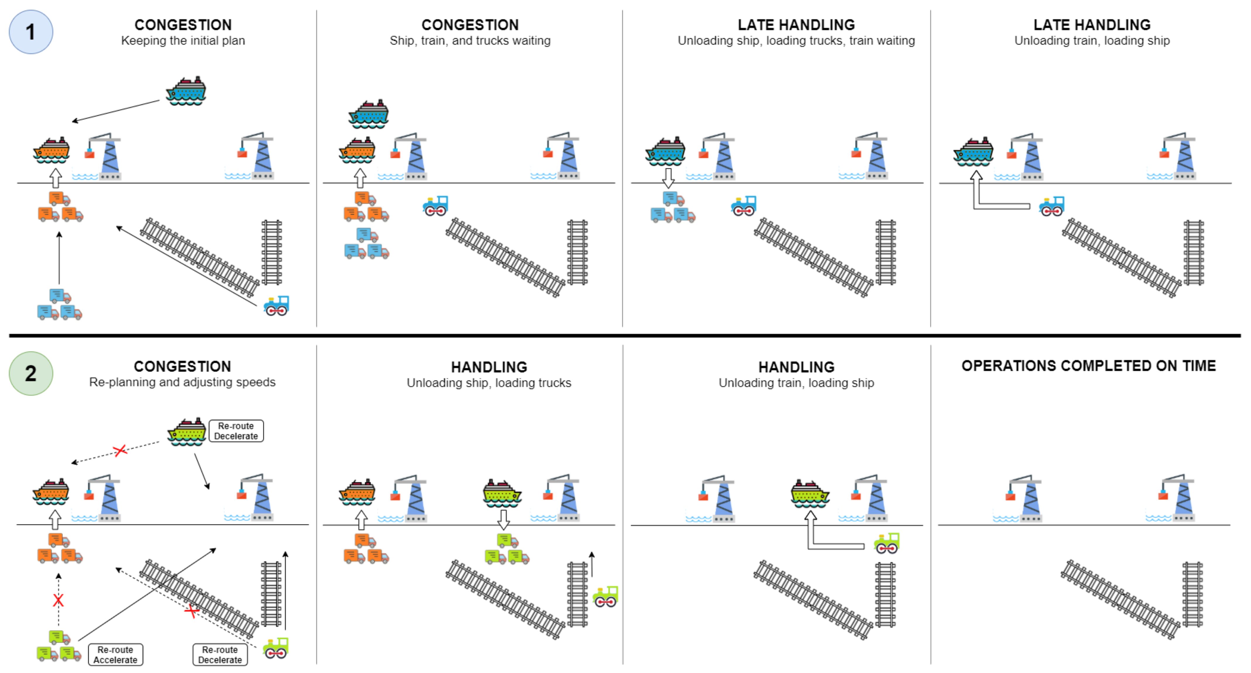
• We presented the paradigm of smart steaming and how it overcomes the current practices’ limits to address synchromodal logistics settings better. Its main features are a global real-time view of the operations and the adoption of re-planning procedures (such as re-routing, re-scheduling, or dynamic speed adjustments).
• We highlighted smart steaming benefits to deal with emissions regulations and the operational limits for its implementation.
• We discussed how to address decision-making problems faced under smart steaming at different planning levels, focusing on handling uncertainty and optimization paradigms.

As smart steaming is a new paradigm, several future research lines arise in many fields. For example, it is crucial to quantitatively estimate (by using rigorous econometric models) how cost-effective smart steaming can be from an economic perspective. This is critical, as companies need to see the advantages of adopting smart steaming to implement it. Moreover, the implementation requires strong cooperation integrating stakeholders’ businesses with common information platforms. This relies on the technical aspects and enormously on how it is possible to manage the business interactions. Concerning this aspect, some possible research questions are as follows: How to manage contracts that include flexible operations? Who is responsible for what in case of disruptions? How to redistribute the gain fairly among stakeholders while focusing on global goals? At what rate costs and emissions may be decreased? How do the number and the expertise of the cooperating stakeholders affect the efficiency, service quality, and sustainability of the logistics network?

Finally, we also believe that decision-making and optimization tools have a decisive role in answering the above questions and providing suitable and reliable solutions both in the long-term and real-time. Therefore, new speed optimization approaches for smart steaming for the different planning levels are required. Developing them is essential to evaluate the smart steaming implementation and later provide tools useful for network design, planning operations, and adopting re-planning procedures. Achieving this goal requires studying deeply the different problems that decision-makers may face under the smart steaming paradigm. Some of the critical questions to address are as follows: How to model the vehicles’ movements and speeds correctly, how to manage problem constraints to provide more flexibility, which objectives should be pursued simultaneously to grasp all the complex aspects of the system?

References

1. Tiwari, S.; Wee, H.M.; Zhou, Y.; Tjoeng, L. Freight consolidation and containerization strategy under business as usual scenario & carbon tax regulation. J. Clean. Prod. 2021, 279, 123270. [Google Scholar]
2. Woo, J.K.; Moon, D.S.H. The effects of slow steaming on the environmental performance in liner shipping. Marit. Policy Manag. 2014, 41, 176–191. [Google Scholar] [CrossRef]
3. Notteboom, T.; Cariou, P. Slow steaming in container liner shipping: Is there any impact on fuel surcharge practices? Int. J. Logist. Manag. 2013, 24, 73–86. [Google Scholar] [CrossRef]
4. Giusti, R.; Manerba, D.; Bruno, G.; Tadei, R. Synchromodal logistics: An overview of critical success factors, enabling technologies, and open research issues. Transp. Res. Part E Logist. Transp. Rev. 2019, 129, 92–110. [Google Scholar] [CrossRef]
5. Perboli, G.; Musso, S.; Rosano, M.; Tadei, R.; Godel, M. Synchro-modality and slow steaming: New business perspectives in freight transportation. Sustainability 2017, 9, 1843. [Google Scholar] [CrossRef] [Green Version]
6. Pfoser, S.; Treiblmaier, H.; Schauer, O. Critical Success Factors of Synchromodality: Results from a Case Study and Literature Review. Transp. Res. Procedia 2016, 14, 1463–1471. [Google Scholar] [CrossRef] [Green Version]
7. Qu, W.; Rezaei, J.; Maknoon, Y.; Tavasszy, L. Hinterland freight transportation replanning model under the framework of synchromodality. Transp. Res. Part E Logist. Transp. Rev. 2019, 131, 308–328. [Google Scholar] [CrossRef]
8. Yin, J.; Fan, L.; Yang, Z.; Li, K.X. Slow steaming of liner trade: Its economic and environmental impacts. Marit. Policy Manag. 2014, 41, 149–158. [Google Scholar] [CrossRef]
9. Maloni, M.; Paul, J.A.; Gligor, D.M. Slow steaming impacts on ocean carriers and shippers. Marit. Econ. Logist. 2013, 15, 151–171. [Google Scholar] [CrossRef] [Green Version]
10. Tai, H.H.; Lin, D.Y. Comparing the unit emissions of daily frequency and slow steaming strategies on trunk route deployment in international container shipping. Transp. Res. Part D Transp. Environ. 2013, 21, 26–31. [Google Scholar] [CrossRef]
11. Tezdogan, T.; Incecik, A.; Turan, O.; Kellett, P. Assessing the Impact of a Slow Steaming Approach on Reducing the Fuel Consumption of a Containership Advancing in Head Seas. Transp. Res. Procedia 2016, 14, 1659–1668. [Google Scholar] [CrossRef] [Green Version]
12. Finnsgård, C.; Kalantari, J.; Roso, V.; Woxenius, J. The Shipper’s perspective on slow steaming—Study of Six Swedish companies. Transp. Policy 2020, 86, 44–49. [Google Scholar] [CrossRef]
13. Meyer, J.; Stahlbock, R.; Voss, S. Slow Steaming in Container Shipping. In Proceedings of the 2012 45th Hawaii International Conference on System Sciences, Maui, HI, USA, 4–7 January 2012; pp. 1306–1314. [Google Scholar]
14. Cariou, P. Is slow steaming a sustainable means of reducing CO2 emissions from container shipping? Transp. Res. Part D Transp. Environ. 2011, 16, 260–264. [Google Scholar] [CrossRef]
15. Psaraftis, H.; Kontovas, C. Slow Steaming in Maritime Transportation: Fundamentals, Trade-offs, and Decision Models. In Handbook of Ocean Container Transport Logistics; Springer: Cham, Switzerland, 2015; pp. 315–358. [Google Scholar]
16. Mander, S. Slow steaming and a new dawn for wind propulsion: A multi-level analysis of two low carbon shipping transitions. Mar. Policy 2017, 75, 210–216. [Google Scholar] [CrossRef]
17. Fan, L.; Huang, L. Analysis of the Incentive for Slow Steaming in Chinese Sulfur Emission Control Areas. Transp. Res. Rec. 2019, 2673, 165–175. [Google Scholar] [CrossRef]
18. Fan, L.; Gu, B. Impacts of the Increasingly Strict Sulfur Limit on Compliance Option Choices: The Case Study of Chinese SECA. Sustainability 2019, 12, 165. [Google Scholar] [CrossRef] [Green Version]
19. Hämäläinen, E. Can slow steaming lower cost impacts of sulphur directive—Shippers’ perspective. World Rev. Intermodal Transp. Res. 2014, 5, 59–79. [Google Scholar] [CrossRef]
20. Raza, Z.; Woxenius, J.; Finnsgård, C. Slow Steaming as Part of SECA Compliance Strategies among RoRo and RoPax Shipping Companies. Sustainability 2019, 11, 1435. [Google Scholar] [CrossRef] [Green Version]
21. Wu, W.M. The optimal speed in container shipping: Theory and empirical evidence. Transp. Res. Part E Logist. Transp. Rev. 2020, 136, 101903. [Google Scholar] [CrossRef]
22. Cepeda, M.F.S.; Assis, L.; Marujo, L.; Caprace, J. Effects of slow steaming strategies on a ship fleet. Mar. Syst. Ocean. Technol. 2017, 12, 178–186. [Google Scholar] [CrossRef]
23. Psaraftis, H.N.; Kontovas, C.A. Balancing the economic and environmental performance of maritime transportation. Transp. Res. Part D Transp. Environ. 2010, 15, 458–462. [Google Scholar] [CrossRef]
24. Ferrari, C.; Parola, F.; Tei, A. Determinants of slow steaming and implications on service patterns. Marit. Policy Manag. 2015, 42, 636–652. [Google Scholar] [CrossRef]
25. Mallidis, I.; Iakovou, E.; Dekker, R.; Vlachos, D. The impact of slow steaming on the carriers’ and shippers’ costs: The case of a global logistics network. Transp. Res. Part E Logist. Transp. Rev. 2018, 111, 18–39. [Google Scholar] [CrossRef] [Green Version]
26. Xiong, Y.; Wang, Z.; Li, D.; Peng, X. Impact Analysis of Slow Steaming on Inland River Container Freight Supply Chain. In Proceedings of the 2018 37th Chinese Control Conference (CCC), Wuhan, China, 25–27 July 2018; pp. 8430–8434. [Google Scholar]
27. Le, L.T.; Lee, G.; Park, K.S.; Kim, H. Neural network-based fuel consumption estimation for container ships in Korea. Marit. Policy Manag. 2020, 47, 615–632. [Google Scholar] [CrossRef]
28. Psaraftis, H. Speed Optimization for Sustainable Shipping. In Sustainable Shipping: A Cross-Disciplinary View; Springer: Berlin/Heidelberg, Germany, 2019; pp. 339–374. [Google Scholar]
29. Lee, C.Y.; Lee, H.L.; Zhang, J. The impact of slow ocean steaming on delivery reliability and fuel consumption. Transp. Res. Part E Logist. Transp. Rev. 2015, 76, 176–190. [Google Scholar] [CrossRef]
30. Reis, V. Should we keep on renaming a +35-year-old baby? J. Transp. Geogr. 2015, 46, 173–179. [Google Scholar] [CrossRef]
31. Van Riessen, B.; Negenborn, R.; Dekker, R.; Lodewijks, G. Service Network Design for an Intermodal Container Network with Flexible due Dates/Times and the Possibility of Using Subcontracted Transport; Econometric Institute Research Papers EI2013-17, Erasmus University Rotterdam, Erasmus School of Economics (ESE), Econometric Institute: Rotterdam, The Netherlands, 2013. [Google Scholar]
32. Ambra, T.; Caris, A.; Macharis, C. Should I Stay or Should I Go? Assessing Intermodal and Synchromodal Resilience from a Decentralized Perspective. Sustainability 2019, 11, 1765. [Google Scholar] [CrossRef] [Green Version]
33. Tavasszy, L.A.; Behdani, B.; Konings, R. Intermodality and Synchromodality. In Ports and Networks; Strategies, Operations and Perspectives; Geerlings, H., Kuipers, B., Zuidwijk, R., Eds.; Routledge: London, UK, 2017; Chapter 16. [Google Scholar]
34. van Riessen, B.; Negenborn, R.R.; Dekker, R. Synchromodal container transportation: An overview of current topics and research opportunities. Lect. Notes Comput. Sci. 2015, 9335, 386–397. [Google Scholar]
35. Dong, C.; Boute, R.; McKinnon, A.; Verelst, M. Investigating synchromodality from a supply chain perspective. Transp. Res. Part D Transp. Environ. 2018, 61, 42–57. [Google Scholar] [CrossRef]
36. Guo, W.; van Blokland, W.B.; Lodewijks, G. Survey on characteristics and challenges of synchromodal transportation in global cold chains. Lect. Notes Comput. Sci. 2017, 10572 LNCS, 420–434. [Google Scholar]
37. Lin, X.; Negenborn, R.R.; Lodewijks, G. Towards Quality-aware Control of Perishable Goods in Synchromodal Transport Networks. IFAC-PapersOnLine 2016, 49, 132–137. [Google Scholar] [CrossRef]
38. Nabais, J.L.; Negenborn, R.R.; Carmona-Benítez, R.; Botto, M.A. Cooperative relations among intermodal hubs and transport providers at freight networks using an MPC approach. Lect. Notes Comput. Sci. 2015, 9335, 478–494. [Google Scholar]
39. Giusti, R.; Iorfida, C.; Li, Y.; Manerba, D.; Musso, S.; Perboli, G.; Tadei, R.; Yuan, S. Sustainable and De-Stressed International Supply-Chains Through the SYNCHRO-NET Approach. Sustainability 2019, 11, 1083. [Google Scholar] [CrossRef] [Green Version]
40. Giusti, R.; Manerba, D.; Perboli, G.; Tadei, R.; Yuan, S. A New Open-source System for Strategic Freight Logistics Planning: The SYNCHRO-NET Optimization Tools. Transp. Res. Procedia 2018, 30, 245–254. [Google Scholar] [CrossRef]
41. Holfeld, D.; Iorfida, C.; Koya, M.; Manerba, D.; Stephens, J.; Tadei, R.; Werner, F. SYNCHRO-NET: A powerful and innovative synchro-modal supply chain eco-NET. In Proceedings of the Transport Research Arena (TRA), Vienna, Austria, 16–19 April 2018. [Google Scholar]
42. Holfeld, D.; Simroth, A.; Li, Y.; Manerba, D.; Tadei, R. Risk Analysis for synchro-modal freight transportation: The SYNCHRO-NET approach. In Proceedings of the Odysseus—7th International Workshop on Freight Transportation and Logistics, Cagliari, Italy, 3–8 June 2018. [Google Scholar]
43. Ben-Chaim, M.; Shmerling, E.; Kuperman, A. Analytic Modeling of Vehicle Fuel Consumption. Energies 2013, 6, 117–127. [Google Scholar] [CrossRef]
44. Zhou, M.; Jin, H.; Wang, W. A review of vehicle fuel consumption models to evaluate eco-driving and eco-routing. Transp. Res. Part D Transp. Environ. 2016, 49, 203–218. [Google Scholar] [CrossRef]
45. Demir, E.; Bektaş, T.; Laporte, G. A comparative analysis of several vehicle emission models for road freight transportation. Transp. Res. Part D Transp. Environ. 2011, 16, 347–357. [Google Scholar] [CrossRef]
46. Heinold, A. Comparing emission estimation models for rail freight transportation. Transp. Res. Part D Transp. Environ. 2020, 86, 102468. [Google Scholar] [CrossRef]
47. Feng, X.; Sun, Q.; Liu, L.; Li, M. Assessing Energy Consumption of High-speed Trains based on Mechanical Energy. Procedia Soc. Behav. Sci. 2014, 138, 783–790. [Google Scholar] [CrossRef] [Green Version]
48. Le, L.T.; Lee, G.; Kim, H.; Woo, S.H. Voyage-based statistical fuel consumption models of ocean-going container ships in Korea. Marit. Policy Manag. 2020, 47, 304–331. [Google Scholar] [CrossRef]
49. Baumel, C.; Hurburgh, C.; Lee, T.; Agriculture, I.; Station, H.E.E. Estimates of Total Fuel Consumption in Transporting Grain from Iowa to Major Grain-importing Countries by Alternative Modes and Routes; Number 77 in Special Report; Iowa State University, Agricultural and Home Economics Experiment Station: Ames, IA, USA, 1985. [Google Scholar]
50. Shobayo, P.; van Hassel, E. Container barge congestion and handling in large seaports: A theoretical agent-based modeling approach. J. Shipp. Trade 2019, 4, 4. [Google Scholar] [CrossRef] [Green Version]
51. Sung, I.; Nielsen, P. Speed optimization algorithm with routing to minimize fuel consumption under time-dependent travel conditions. Prod. Manuf. Res. 2020, 8, 1–19. [Google Scholar] [CrossRef] [Green Version]
52. Zhao, Y.; Zhou, J.; Fan, Y.; Kuang, H. An Expected Utility-Based Optimization of Slow Steaming in Sulphur Emission Control Areas by Applying Big Data Analytics. IEEE Access 2020, 8, 3646–3655. [Google Scholar] [CrossRef]
53. Yuzhe, Z.; Zhou, J.; Fan, Y.; Kuang, H. Sailing Speed Optimization Model for Slow Steaming Considering Loss Aversion Mechanism. J. Adv. Transp. 2020, 2020. [Google Scholar] [CrossRef]
54. Wong, E.Y.; Tai, A.H.; Lau, H.Y.; Raman, M. An utility-based decision support sustainability model in slow steaming maritime operations. Transp. Res. Part E Logist. Transp. Rev. 2015, 78, 57–69. [Google Scholar] [CrossRef]
55. Li, X.; Sun, B.; Guo, C.; Du, W.; Li, Y. Speed optimization of a container ship on a given route considering voluntary speed loss and emissions. Appl. Ocean. Res. 2020, 94, 101995. [Google Scholar] [CrossRef]
56. Tezdogan, T.; Demirel, Y.; Kellett, P.; Khorasanchi, M.; Incecik, A.; Turan, O. Full-scale unsteady RANS CFD simulations of ship behaviour and performance in head seas due to slow steaming. Ocean. Eng. 2015, 97, 186–206. [Google Scholar] [CrossRef] [Green Version]
57. Rahman, A.; Yang, Z.; Bonsall, S.B.; Wang, J. A Proposed Rule-based bayesian Reasoning Appoarch for Analysing Steaming Modes on Containerships. J. Marit. Res. 2012, 9, 27–32. [Google Scholar]
58. Wang, H.; Lang, X.; Mao, W.; Zhang, D.; Storhaug, G. Effectiveness of 2D optimization algorithms considering voluntary speed reduction under uncertain metocean conditions. Ocean. Eng. 2020, 200, 107063. [Google Scholar] [CrossRef]
59. Bektaş, T.; Laporte, G. The Pollution-Routing Problem. Transp. Res. Part B Methodol. 2011, 45, 1232–1250. [Google Scholar] [CrossRef]
60. Kumar, R.S.; Kondapaneni, K.; Dixit, V.; Goswami, A.; Thakur, L.; Tiwari, M. Multi-objective modeling of production and pollution routing problem with time window: A self-learning particle swarm optimization approach. Comput. Ind. Eng. 2016, 99, 29–40. [Google Scholar] [CrossRef]
61. Ren, X.; Huang, H.; Feng, S.; Liang, G. An improved variable neighborhood search for bi-objective mixed-energy fleet vehicle routing problem. J. Clean. Prod. 2020, 275, 124155. [Google Scholar] [CrossRef]
62. Eshtehadi, R.; Fathian, M.; Demir, E. Robust solutions to the pollution-routing problem with demand and travel time uncertainty. Transp. Res. Part D Transp. Environ. 2017, 51, 351–363. [Google Scholar] [CrossRef]
63. Tirkolaee, E.B.; Goli, A.; Faridnia, A.; Soltani, M.; Weber, G.W. Multi-objective optimization for the reliable pollution-routing problem with cross-dock selection using Pareto-based algorithms. J. Clean. Prod. 2020, 276, 122927. [Google Scholar] [CrossRef]
64. Hoen, K.M.R.; Tan, T.; Fransoo, J.C.; van Houtum, G.J. Effect of carbon emission regulations on transport mode selection under stochastic demand. Flex. Serv. Manuf. J. 2014, 26, 170–195. [Google Scholar] [CrossRef] [Green Version]
65. An, S.; Li, B.; Song, D.; Chen, X. Green credit financing versus trade credit financing in a supply chain with carbon emission limits. Eur. J. Oper. Res. 2020, 292, 125–142. [Google Scholar] [CrossRef]
66. Tsao, Y.C. Design of a carbon-efficient supply-chain network under trade credits. Int. J. Syst. Sci. Oper. Logist. 2015, 2, 177–186. [Google Scholar] [CrossRef]
67. Baranzini, A.; Goldemberg, J.; Speck, S. A future for carbon taxes. Ecol. Econ. 2000, 32, 395–412. [Google Scholar] [CrossRef]
68. Rotaris, L.; Danielis, R. The willingness to pay for a carbon tax in Italy. Transp. Res. Part D Transp. Environ. 2019, 67, 659–673. [Google Scholar] [CrossRef]
69. McHale, M.R.; Gregory McPherson, E.; Burke, I.C. The potential of urban tree plantings to be cost effective in carbon credit markets. Urban For. Urban Green. 2007, 6, 49–60. [Google Scholar] [CrossRef]
70. Narassimhan, E.; Gallagher, K.S.; Koester, S.; Alejo, J.R. Carbon pricing in practice: A review of existing emissions trading systems. Clim. Policy 2018, 18, 967–991. [Google Scholar] [CrossRef] [Green Version]
71. Bialystocki, N.; Konovessis, D. On the estimation of ship’s fuel consumption and speed curve: A statistical approach. J. Ocean. Eng. Sci. 2016, 1, 157–166. [Google Scholar] [CrossRef] [Green Version]
72. Notteboom, T.E.; Vernimmen, B. The effect of high fuel costs on liner service configuration in container shipping. J. Transp. Geogr. 2009, 17, 325–337. [Google Scholar] [CrossRef]
73. Kruse, C.J.; Warner, J.E.; Olson, L.E. A Modal Comparison of Domestic Freight Transportation Effects on the General Public: 2001–2014; Technical Report; Texas A&M Transportation Institute: Bryan, TX, USA, 2017. [Google Scholar]
74. King, A.J.; Wallace, S. Modeling with Stochastic Programming; Springer Series in Operations Research and Financial Engineering; Springer: New York, NY, USA, 2012. [Google Scholar]
75. Crainic, T.G.; Giusti, R.; Manerba, D.; Tadei, R. The Synchronized Location-Transshipment Problem. Transp. Res. Procedia 2021, 52, 43–50. [Google Scholar] [CrossRef]
76. Giusti, R.; Manerba, D.; Tadei, R. Multiperiod transshipment location–allocation problem with flow synchronization under stochastic handling operations. Networks 2020. [Google Scholar] [CrossRef]
77. Birge, J.R.; Louveaux, F.V. Introduction to Stochastic Programming; Springer: New York, NY, USA, 1997. [Google Scholar]
78. Ben-Tal, A.; Ghaoui, L.E.; Nemirovski, A. Robust Optimization; Princeton University Press: Princeton, NJ, USA, 2009. [Google Scholar]
79. Hrus̆ovský, M.; Demir, E.; Jammernegg, W.; Van Woensel, T. Real-time disruption management approach for intermodal freight transportation. J. Clean. Prod. 2021, 280, 124826. [Google Scholar] [CrossRef]
80. Jaillet, P.; Wagner, M.R. Online Optimization—An Introduction. In Risk and Optimization in an Uncertain World; INFORMS: Catonsville, MD, USA, 2010; Chapter 6; pp. 142–152. [Google Scholar]
81. Puterman, M.L. Markov Decision Processes: Discrete Stochastic Dynamic Programming; John Wiley & Sons, Inc.: Hoboken, NJ, USA, 1994. [Google Scholar]
82. Hentenryck, P.V.; Bent, R. Online Stochastic Combinatorial Optimization; The MIT Press: Cambridge, MA, USA, 2006. [Google Scholar]
Figure 1. Evolution of freight transportation, from multimodality to synchromodality.
Sustainability 13 04635 g001
Figure 2. Comparison of following a static strategy (blue ship) with adopting smart steaming (green ship). The two ships have the same speed, but the green one detects congestion at its destination port. The green ship decelerates, whereas the blue one continues at the same speed, producing 20 tons of CO 2 . Moreover, it arrives when the port is still congested. Slowing down the green ship produces less CO 2 (15 tons in total) and is handled without idle time.
Sustainability 13 04635 g002
Figure 3. Comparison of a logistics network following a static strategy (blue vehicles) with one adopting synchromodality and smart steaming (green vehicles). The initial plan (dashed arrows with a red cross) is adjusted differently for all the green vehicles, making possible to finish operations on time.
Sustainability 13 04635 g003
Publisher’s Note: MDPI stays neutral with regard to jurisdictional claims in published maps and institutional affiliations.