Article

Application of Artificial Neural Networks to Streamline the Process of Adaptive Cruise Control

1
Department of Mechanical and Electrical Engineering, ŠKODA AUTO University, 1457, 29301 Mladá Boleslav, Czech Republic
2
Department of Quantitative Methods, ŠKODA AUTO University, 1457, 29301 Mladá Boleslav, Czech Republic
*
Author to whom correspondence should be addressed.
Sustainability 2021, 13(8), 4572; https://doi.org/10.3390/su13084572
Submission received: 16 February 2021 / Revised: 9 April 2021 / Accepted: 12 April 2021 / Published: 20 April 2021
(This article belongs to the Special Issue Green ICT, Artificial Intelligence and Smart Cities)

Abstract

:
This article deals with the use of neural networks for estimation of deceleration model parameters for the adaptive cruise control unit. The article describes the basic functionality of adaptive cruise control and creates a mathematical model of braking, which is one of the basic functions of adaptive cruise control. Furthermore, an analysis of the influences acting in the braking process is performed, the most significant of which are used in the design of deceleration prediction for the adaptive cruise control unit using neural networks. Such a connection using artificial neural networks using modern sensors can be another step towards full vehicle autonomy. The advantage of this approach is the original use of neural networks, which refines the determination of the deceleration value of the vehicle in front of a static or dynamic obstacle, while including a number of influences that affect the braking process and thus increase driving safety.

1. Introduction

Today, modern cars are equipped with intelligent systems. These are systems that should make it easier for drivers to control the vehicle, increase driving comfort and traffic safety. Emerging car technologies today work more closely with the driver and are more interactive. Very often a touch screen or human voice control is used.
Intelligent systems fall into two categories. The first category is IN Vehicle Information Systems (INVIS) information systems. These include various navigation and communication systems such as the on-board computer, mobile phone, navigation and car radio. The second category is Advanced Driver Assistance Systems (ADAS). These help drivers in various traffic situations either by warning the driver or by taking control of individual vehicle functions.
Advanced safety assistance systems directly intervene in the steering. The aim is to reduce human-made driving requirements, eliminate possible driver errors and improve the economic aspects of driving. However, no safety assistance system relieves the driver of responsibility for safety and driving. Adaptive cruise control is now used to maintain a safe distance. The driver can then pay more attention to other aspects of the traffic situation. The aspect of increasing safety was the motivation for the research of the application of artificial neural networks for the system of adaptive cruise control.
The aim of the article is to show the possibilities of application of neural networks as a new concept of functionality of the car assistance system, which will connect the possibilities of modern sensors and artificial intelligence to increase driving safety, which is the basis for the transition to autonomous vehicles.
The novel contributions of the article are
  • design of a completely original hierarchical neural network representing the control core of adaptive cruise control;
  • application of neural networks to determine the deceleration value of a vehicle in front of a static or dynamic obstacle based on traditional and non-traditional input factors that affect the braking process;
  • at the same time, it is another presentation of the use of artificial neural networks and modern sensors on the way to full vehicle autonomy.
Several approaches have been proposed, for example [1,2,3], to automatically monitor the condition of the road surface in order to improve driving parameters. These solutions are inspiring and also use artificial neural networks but are focused on the optimization of the anti-lock brake system (ABS) [1] or only propose technical solutions [2,3]. The proposed solution in the article represents a comprehensive approach, which is focused on adaptive cruise control (ACC), i.e., primarily on ensuring safety, including the effects of safe braking or deceleration. The introduction of the article and chapter 2 outline the importance of new technologies in automobiles for the sustainable development of humanity and the development of transport systems leading to autonomous management. Chapter 3 is devoted to assistance systems in the car with a focus on adaptive cruise control, which is described in terms of its architecture, principle and its main function—speed stabilization. Chapter 4 of the article presents a simplified mathematical model of deceleration of a vehicle in front of an obstacle, which is the basis for the main part of the article—chapter 5—design of a hierarchical neural network as a means to intelligently support safe driving and which uses traditional and non-traditional factors influencing the safe braking process. Part of the research attention was paid mainly to the aspect of safety, but it can be assumed that it will also affect the areas of fuel consumption and emissions. The research was based on a search of the topic, the partial conclusions of which are given at the end of Chapter 3.1 and which show that the chosen solution is unique in this area, but must be supplemented by technical solutions and a number of experimental tests.
Sustainable development is based on the application of modern methods and tools, to which artificial intelligence belongs. Mobility and thus transport systems significantly affect the social, economic and environmental areas of society, both positively and negatively. New methods and technologies should allow us to find the optimum, i.e., to strengthen the positive aspects and eliminate the negative ones. These changes will not be a leap, but any contribution devoted to the application of new and modern technologies, such as artificial intelligence, is a step that brings society closer to this optimum.

2. The Impact of New Technologies on Sustainability in Cars

The ongoing 4th Industrial Revolution focuses on the application of scientific knowledge not only to industrial production, but also in everyday life, including in the automotive field. Modern materials and technologies aim to significantly improve the driving and technical properties of cars, which is an example of the above-described application of artificial neural networks within the system of adaptive cruise control.
The automotive industry is one of the important areas of application of modern technologies—auto electrification, autonomous management, applications based on the Internet of Things, digitization, predictive and prescriptive diagnostics, which manifest themselves in the context of overall sustainability. These technologies assume a departure from conventional applications, for example in the field of internal combustion engine production; on the other hand, development is expected in the field of human machine interface and electrical components of cars. These trends, together with the company’s concept of sustainable development, are an appeal for the development of new technologies, materials and technical solutions. In the case of electric cars, they help to extend the travel time.
All these technologies aim to achieve the principles of sustainable mobility, which is based on the paradigm of sustainable development. This means development that meets the needs of current generations without risking that the needs of future generations cannot be met. If we study sustainable mobility, it is interesting that the number of trips a person makes per day on average does not change in the long run (e.g., in the last 50 years) and the time spent on them does not change. This is related to the development of human society and technical development—we still travel for work, shopping, hobbies, trips, etc., cars allow us to cover longer distances, but the distance of our targets and the speed of used vehicles increases significantly. Thus, better communication in the long run does not allow people to spend less time on the road, but rather to travel longer distances, at higher costs and with greater negative impacts on the environment. A source [4] states that a 20% reduction in driving time will lead to a 10% increase in traffic intensity in the short term and a 20% increase in the long term.
Thus, we can consider an efficient transport system that allows people to satisfy their needs at the lowest social cost. The sample list for individual car transport is very long: traffic accidents (direct economic consequences, health consequences, police, health service, fire brigade, liquidation of environmental impacts, etc.), noise, air pollution, costs caused by climate change, impact on nature and landscape (landscape fragmentation—impact on animal populations, risk of spreading invasive plant species along the road), costs incurred earlier or subsequently (car production, ecological disposal), reducing the attractiveness of the area, additional costs in the urban environment and more.
In addition, a number of negative but also positive factors are very difficult to quantify purely in economic categories. Some of the factors within sustainable mobility are transformed into the so-called ecological footprint, which is a measure of human demand for the earth’s ecosystem (measured in so-called global hectares per person). In principle, these are negative factors affecting the environment, converted to individuals, depending on how and how far they are transported.
The mere fact that transport is part of the economic system (and brings, for example, job opportunities) cannot be considered a positive factor. By delaying their targets, people are forced to pay more for transport than they would like. If they paid less for transportation, they would save the money saved to better meet their needs. The aim of transport is primarily the transport of people and goods. It is true that transport is one of the four main sectors of the economy (the rest are households; mining and processing; services and other industries), which cannot be underestimated, but the economic performance of the transport sector must always be measured by negative factors, which are usually not compensated for. Additionally, it is new technologies, for example based on artificial intelligence leading to autonomous mobility, that can significantly influence a number of the above-mentioned factors.
Currently, we observe two main directions in the automation of car driving [5], these are the so-called assistance systems and automatic highway, which are different, but complement and influence each other, because development in one direction automatically means progress in the other direction as well. The principle and concept of the automatic motorway focuses on the complete automation of the driver’s function (Figure 1): when crossing the boundary of the automated section of the road, the driver marks the destination of his route determining the end point on the automated section [6]. Subsequently, the car takes over all the functions of driving the car and the driver has the opportunity to perform other activities at his discretion. As soon as the car reaches the end point of the exit from the automated section of the road, the car notifies the driver of this fact and the automatic mode is terminated and the driver takes over the driving. The system of the automatic highway has been complete for several years and from the technical point of view its solution is almost complete [7].
The basic problem for implementation in practice is still almost insurmountable legislative problems. It has not been determined by law who is responsible for the movement of the car and thus for the consequences of failure in the event of an accident caused by the failure of the automatic system. An automatic system is a technical device, but not a legal entity taking on legal consequences. If the automatic motorway system is to be implemented in practice, this requires significant adjustments and changes in legislation.
Simultaneously with the development of the automatic motorway, so-called assistance systems are being developed [8]. Assistance systems assist the driver in specified activities and situations. They help him, but unlike the automatic highway system, full responsibility for driving and all the consequences and mistakes remains with the driver. Assistance systems are designed to support safe and fast driver decisions when driving a car.

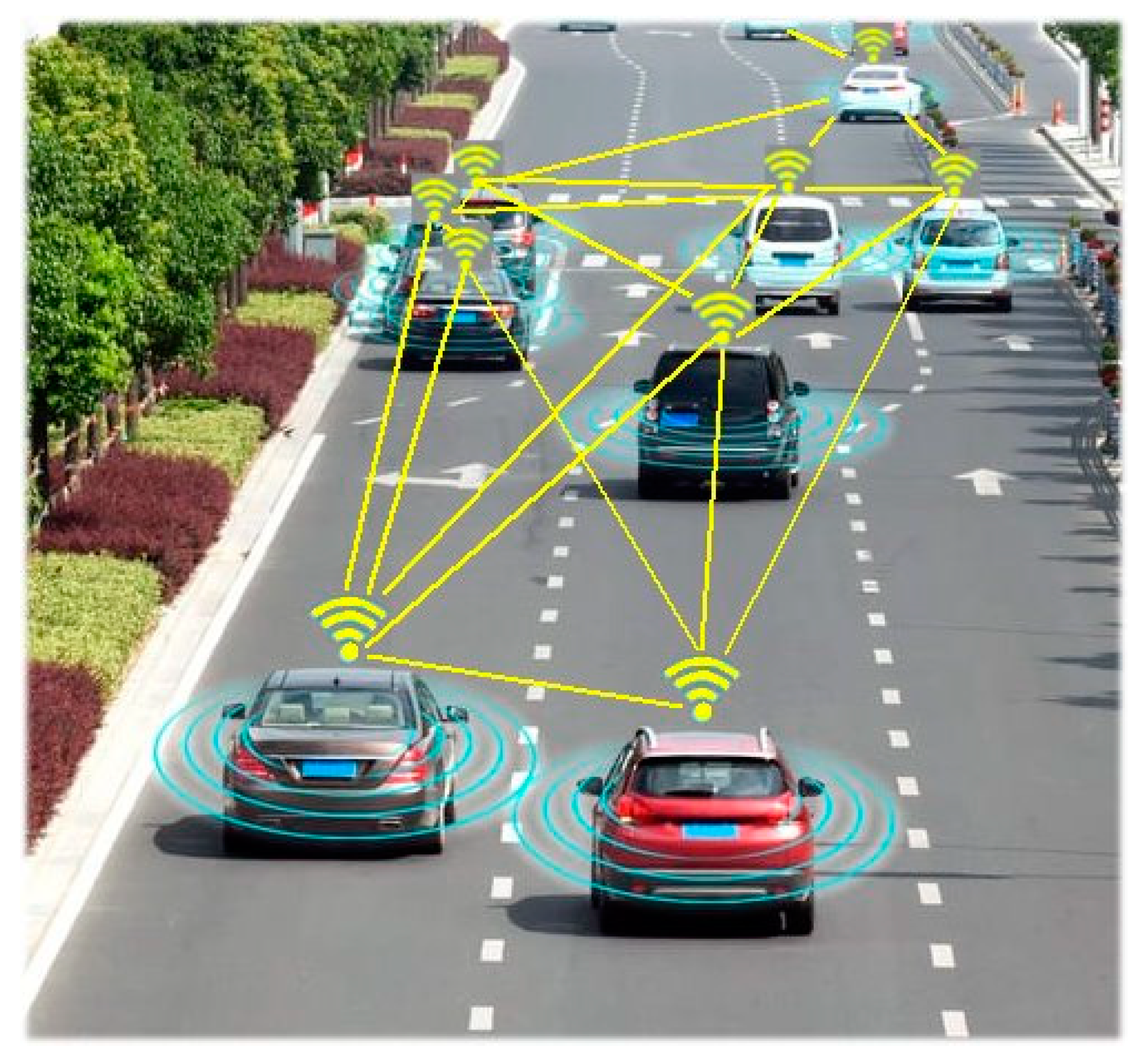
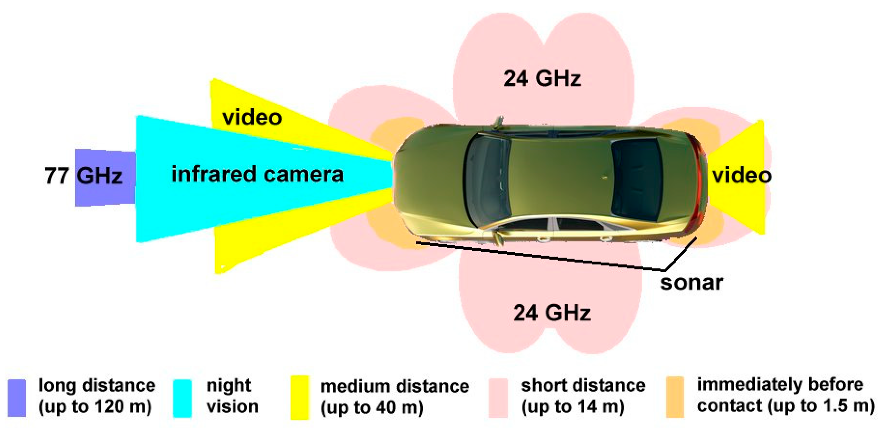
3. Assistance Systems in Cars

Development and implementation of a complete car control system in the sense of an autonomous car is possible only through the decomposition of the entire complex control system into partial separate control tasks, which are well described and which then perform the function of an assistance system such as directional control (longitudinal control), position maintenance in the lane (transverse control), speed and acceleration control, obstacle warning, navigation, etc.

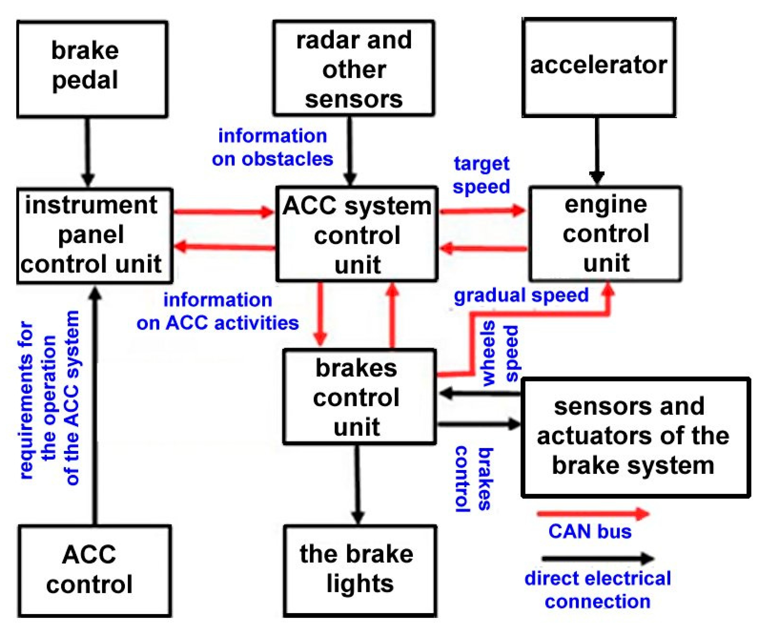
3.1. Adaptive Cruise Control

Adaptive Cruise Control (ACC) is the most common system for improving visibility that interferes with vehicle speed. The difference between conventional cruise control and adaptive cruise control is that conventional cruise control acts as a mere speed controller on the free road and maintains a constant car speed, unlike adaptive cruise control, which monitors the condition in front of the car and a moving obstacle (car); it reaches a predetermined distance, which it then maintains (i.e., adjusts the speed of the car to the speed of the car in front of it). If adaptive cruise control indicates a standing obstacle, it stops at a safe distance in front of the obstacle [9].
The sensors and technical means used by the directional adaptive cruise control system can also be directed backwards and to the sides, as well as for the driver to a “blind” angle. Information and signals from these sensors can give the driver early warning of the possibility of collisions, or give impetus to the automatic execution of a collision warning system (Collision Warning Systems—CWS, Collision Avoidance Systems—CAS).
A number of sensors are used in adaptive cruise control (ACC) systems of various versions (from simple cruise control to anti-collision systems). Their ranges and radiation diagrams are schematically shown in Figure 2 [10]. The microwave radar operates at a frequency of 77 GHz and has the longest range and is able to detect an obstacle at a distance of about 120 m in front of the car. Another sensor is an infrared camera, whose range is comparable. The video camera working in the visible part of the spectrum has a useful range of about 40 m. The surroundings up to 15 m of the car are monitored by microwave radars operating at a frequency of 24 GHz and are mainly used by anti-collision systems. For the immediate surroundings and in the event of a collision, there are ultrasonic (sonar) sensors with a range of approx. 1 m at the front and rear, which are used to activate protective devices (belt tightening, airbag deployment) if a collision can no longer be avoided.
The most important sensor for the operation of the ACC system is a radar operating at a frequency of 77 GHz with a relatively narrow radiation pattern, which registers an obstacle at a large distance and at the same time identifies its speed (Figure 3) [11]. On a straight road, only this radar would be sufficient for driving, but in heavy traffic and in bends, it is necessary to supplement it with an infrared camera, or video cameras operating in the visible area, which are connected to a computer enabling image processing and thus constantly capture and evaluate the traffic situation in front of the car.
In addition to radar sensors, an important part of the ACC system is a control unit with situation analysis software, which basically solves the following four situations:
  • It maintains a constant speed on empty communication. The ACC then works as a classic controller, sending a setpoint of engine speed to the engine control unit in a car with an automatic transmission.
  • If a moving obstacle is identified (a car traveling in the same lane at a lower speed), the ACC moves the car to a preset distance, adapts its speed to the car in front and follows it, including in convoys and city traffic.
  • In the case of identification of a stationary obstacle (parked car), the ACC system gradually decreases the speed, so it stops at the optimal distance in front of it.
  • If an obstacle is identified late or suddenly appears in front of the car and the distance from it is shorter than the distance for gradual stopping, the ACC system activates anti-collision systems.
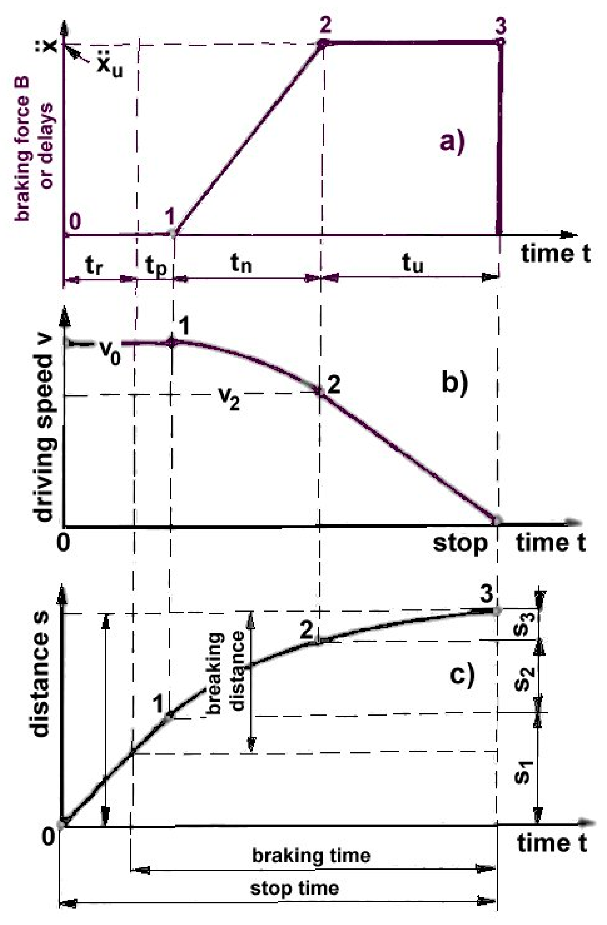
In the above situations, the ACC control unit actively cooperates with the engine control units and the brake control unit. This arrangement is shown in Figure 4. The intensity of cooperation of these systems depends on the ACC regime. The ACC system is designed so that whenever the driver intervenes (braking, accelerating), it automatically disconnects and transfers control to the human operator, which is not the case if the situation requires the activation of anti-collision systems [12,13].
The problem of adaptive cruise control (ACC) can be transformed into the problem of optimal tracking control for complex nonlinear systems. This task is currently solved by different methods using different methods—for example with experience playback technology [14], neural networks [15,16,17,18,19,20,21,22,23,24,25,26,27,28], fuzzy-neural approaches [29,30,31], adaptive algorithms [32,33], or combinations thereof [34,35,36] or modern function approximation techniques together with gradient learning algorithms [37].
Publications describing the use of neural networks [15,16,17,18,19,20,21,22,23,24,25,26,27] mostly apply them as a model of driver behavior [15,19,20,21,22,23,27], which is connected to the ACC assistance system. The aim is to create a driver model imitating the driver’s activity based on real data and their analysis. Algorithms for collision warning and automatic braking are designed based on the timing of the driver’s pedal being depressed when approaching a vehicle or obstacle. Using these experimental studies, the parameters of the driver model can be identified from the data in the manual operation phase, and the identification result is used during the real-time automatic control phase.
Another group of publications [16,18,25,26,28] is the application of neural networks in ACC internal control loops and have the function of a predictive control algorithm that integrates the ability of artificial neural networks to mimic vehicle characteristics and predictive model control to minimize quadratic error between future reference trajectories and predicted outputs. In many cases, two separate control loops are used: an outer loop based on a decision algorithm and a continuous controller that gives the inner loop a reference speed to maintain a safe distance from the vehicle in front. The neural network is then used in the inner loop to manipulate the gas and brake pressure on the brakes to control the speed of the next vehicle.
The last group—the minority [17,24] is the use of neural networks in this area with the aim of how intelligent vehicles equipped with adaptive cruise control improve the efficiency and safety of the highway in bottlenecks. Neural networks obtain lane change characteristics based on vehicle trajectory data showing how the vehicle’s trajectory affects and is affected by road capacity and traffic safety.
Neural networks represent an unconventional approach to modeling various processes and in many cases replace regression methods [38,39]; their advantage is that their nonlinear approach can significantly imitate reality better than regression methods, as shown by Figure 5 [40], representing the steam consumption model in time with categorical variables.
Modern technologies such as ACC require the use of modern tools. Each of the mentioned articles approaches ACC control in a different way and solves various sub-tasks of ACC control (lane-to-lane changeover, automatic control as the basis of an unmanned vehicle, optimization of power and fuel consumption, driving in a convoy, etc.). In contrast to the cited ones, the presented article is defined by focusing on the role of braking, respectively determining the deceleration of a vehicle to ensure safe driving, which in real driving is a complex function affected by a number of driving factors. The solution of such a problem is suitable by means of a hierarchical neural network, which is presented below (chapter 5.2) and which is unique in this area. The presented solution can be another step to streamline the function of adaptive cruise control and also another step towards the full autonomy of the vehicle, where a safe stop in front of an obstacle is one of the basic tasks.
Current electronic assistance systems are set up to make driving more enjoyable, safer and keep the driver in a good condition. Cruise control maintains the selected pace, which is comfortable, safe and very economical on straight sections. Cruise control is designed to maintain constant speed and distance in all conditions, which does not mean that it is always economical (reduction in fuel consumption) and therefore ecological (reduction in CO2 emissions). If cruise control is to have a safety, economic and environmental function, this means further research and development. Already the next stage of development is predictive cruise control to predict and respond to the situation in front of the vehicle (traffic restrictions, track profile, etc.), another evolution of cruise control, then the connection with an ECO mode can be a solution for not only safety but also optimization of consumption and environmental impact. Here, too, artificial intelligence can be a tool for solving these tasks.

3.2. Braking

Speed control within the ACC activity is related to the act of braking, which is understood here as a purposeful speed reduction. Service braking of road vehicles is usually carried out (not for all vehicles) on all wheels. Vehicles are usually driven only on some wheels. In the following diagrams (Figure 6) [41] they are shown as a function of time. We divide braking into several stages. The first is called the reaction time tr. It is the time that elapses between the observation of an obstacle and the time when we start to act on the brake pedal. The next time is called the reaction tp, it is the time before the braking effect starts to show, it can also be called the brake delay. During this time, the play and the brake lining must be defined; they must rest on the friction surface of the brakes, which can be a brake disc or another part, depending on the design of the brake system. During this time, the speed hardly changes and a certain distance is traveled in this section. The next part is called the start of braking tn, which is the time from the beginning of the brakes to the maximum braking, in which the braking force increases. The next section is full braking tu, where we assume that the delay is constant. This braking is until the car comes to a complete stop or until the brake pedal is released [41].
The path to stop is important when controlling ACC operation. It is the distance the vehicle travels from the time of observation of a static obstacle to a complete stop, respectively the distance traveled by the vehicle from the time the dynamic obstacle is observed until the preset safe distance from that obstacle is reached and adapted to its speed.

4. Mathematical Model of Vehicle Movement

In terms of system procedures in creating a mathematical model to support ACC control, the basis is the definition of a controlled system and the identification of essential variables that describe the behavior of the system or affect it (Figure 7) [42]. Each object has a certain shape and structural properties (S1 and S5), has an environment (S0) in which it occupies a certain position and has connections with the environment (S2). Through links, interactions take place in the form of activation (S3) or influence (S4). Furthermore, the processes change the states of the object (S6). The object somehow manifests itself externally (S7), which has some consequences (S9). From a practical point of view, it is necessary to investigate the effect of changing more input variables in a technically acceptable range on the results of output variables [42].
When analyzing moving objects (vehicles) that are in contact with the road, the coefficient of adhesion f (-) between the road surface or surroundings (asphalt, concrete, grass, snow) and the colliding element, i.e., the tire (drag friction coefficient, usually marked as f (-)), is very important. [42].
Adhesion is therefore the ability of a material (especially two different materials) to adhere to one another, more professionally physically it is the ability to transmit tangential forces at the contact of two surfaces without distinct movement. Unlike friction, vehicle adhesion also includes other resistances [42]. The distribution of the forces acting on the vehicle during braking is shown in the following Figure 8 [43].
Mathematical–physical analysis of vehicle motion and braking process generally interweaves the so-called Newton’s laws of motion, which were formulated as equations of motion for mass points and generalized for rigid bodies:
  • law of inertia;
  • law of force;
law of action and reaction and conservation laws:
  • energy;
  • momentum;
  • momentum (rotation).
The basic model describing driving and braking is given below.
Let us introduce parameters and physical quantities describing the problem (see Figure 9). Let d(t) be the positive instantaneous distance between a vehicle and a standing obstacle denoted O at time t, v(t) non-negative instantaneous speed and a(t) absolute value of the instantaneous deceleration of the vehicle. For moving objects O the following holds true if v(t) is the relative instantaneous velocity with respect to O. Using time derivatives denoted with primes it holds for each time t ∈ (0; τ) and decreasing distance d(t)
v ( t ) = d ( t ) 0 ,
a ( t ) = v ( t ) = d ( t ) 0 .
Function d(t) is always a non-concave function. Functions v(t) and a(t) may be convex, concave, or linear. Let us suppose that braking was initiated at the time t = 0 and the distance d(0) = d0 while the speed of a car was v(0) = v0. Finally, let us introduce a security parameter dmin specifying the minimum distance in front of the obstacle where the car has just to stop. Therefore, d0, dmin, and v0 is the minimum set of input parameters for the simplest case. Our goal is to find the optimum velocity v(t) as a function of time t ∈(0; τ) describing the motion until the car has stopped at the time τ.
Before more complex discussion, we should consider linearly decreasing function
v(t) = v0alin t
where constant deceleration alin might be regarded as a secure way of emergency stopping at time τlin. In this case braking distance corresponds to the expression in brackets in Equation (4):
d ( τ lin ) = d min = d 0 ( v 0 τ lin 1 2 a lin τ lin 2 ) ,
v ( τ lin ) = 0 = v 0 a lin τ lin .
Solution to the system of two equations above is
τ lin = 2 ( d 0 d min ) v 0 2 ,   a lin = v 0 τ lin = v 0 2 2 ( d 0 d min ) .
In general, fixed braking distance L = d0dmin that corresponds to the slowdown/stopping period of time τ (i.e., v(τ) = 0) is given by the integral in Equation (7) of the following system:
d 0 d min d d = 0 τ v ( t ) d t = d min d 0   d 0 d min = 0 τ v ( t ) d t ,
v 0 v ( τ ) d v = v ( τ ) v 0 = 0 τ a ( t ) d t   v ( τ ) = v 0 0 τ a ( t ) d t = 0   v 0 = 0 τ a ( t ) d t .
Instantaneous values of both v(t) and a(t) can be obtained from vehicle sensors. In this case the secure minimum distance dmin should be greater than total error given with worst possible uncertainties of the sensor readings.
In further discussion, we can assume continuous non-convex and non-negative functions a(t) satisfying boundary conditions
a(0) = a(τ) = 0, v(0) = v0, v(τ) = 0
which may be considered to be comfortable enough for car slowdown. Maximum instantaneous deceleration a(t) should not exceed a threshold value amax, which is set with a view to ensuring safe driving (i.e., minimizing the risk of the car skidding due to braking and further injuring the car occupants due to braking) and that is proportional to an effective coefficient of static friction f and gravity acceleration g = 9.81 m⋅s−2
a ( t ) a max f · g   for   each   t ( 0 ; τ ) .
The proposed full set of input parameters in our approach includes d0, dmin, v0, and amax. Moreover, corresponding values of alin and τlin from Equation (6) might also be taken into consideration [44].
These are mainly relations for the calculation of the path, time and speed of uniform and accelerated or decelerated rectilinear (rotational) motion. These relationships allow trajectory–time analysis, i.e., a simplified mathematical–physical description of the dynamics of the process of braking objects in a single time.

5. Use of Neural Networks to Support ACC Control

Although neural technologies are very promising and open up many application possibilities where existing information technologies have encountered difficulties or failed completely, in many practical cases approaches that merge conventional and neural technologies are preferred. However, there are areas where this technology brings fundamental benefits. These are mainly tasks related to the processing of incomplete, inaccurate, contradictory and indeterminate information, regression tasks, predictions, classification tasks, recognition of complex signals and images, tasks of an optimizing nature under difficult, often time-varying conditions. It is mainly a solution to problems where a clear solution algorithm is not known, but there is a fairly large set of examples whose solution is known.
Neural networks have proven to be suitable for modeling such real systems, which are characterized by considerable complexity and great difficulty of mathematical description. They are particularly suitable for “self-learning” unstructured data with a high degree of nonlinearity and a high degree of uncertainty [11]. They offer an interesting alternative approach to classical laborious methods of evaluating statistical data, such as regression analysis. At the same time, they are able to capture much more complex relationships than these methods.
The most common objections to neural networks are based on the incomprehensible way in which they represent the knowledge stored in them. In the large matrices of scales, the laws found are stored in such a distributed way that they are “invisible”. Another disadvantage of neural networks is the uncertainty as to whether the desired results can be achieved, as well as the fact that it is not possible to estimate in advance the magnitude of the error, which depends on the network parameters and the training set.
The task of determining the deceleration of a vehicle, where in real driving there is a deceleration of functions, which is influenced by a number of factors discussed above, represents a task which is particularly suitable for solutions using neural networks. This task can be another step towards streamlining the adaptive cruise control function as well as another step from full vehicle autonomy, where safe stopping in front of an obstacle is one of the basic tasks. From the above mathematical–physical analysis of the braking process, it is clear that this is a complex process that requires a large number of sensor systems that could correctly quantify the parameters. The following text shows how neural networks could work with such quantitatively expressed parameters and predict the deceleration value of the vehicle based on them and provide this value to the ACC control unit.

5.1. Adhesion

The achievable deceleration of the vehicle during intensive braking is mainly due to two completely independent parameters, the influence of which can be clearly explained.
In a specific case, usually only one of these two parameters applies.
  • Efficiency of vehicle brakes. Therefore, a road with extremely good anti-skid properties will make the road rougher than usual, saving nothing if the brakes are ineffective (greasy or otherwise broken) on the vehicle. In this case, the anti-slip qualities of the road surface cannot be used.
  • Tire adhesion on the road. Extraordinary effectiveness of the brakes does not save anything on slippery roads (wet, extremely smooth, muddy or icy). In this case, the effectiveness of the brakes simply cannot be used, even if the passenger car has brakes from a large transport aircraft.
Other important circumstances which it is absolutely necessary to distinguish and be focused on are:
  • adhesive requirements;
  • adhesion options.
It is necessary to realize that the adhesion requirements cannot exceed the adhesion possibilities, i.e., driving in which adhesion requirements are placed above the adhesion possibilities means a loss of control of the vehicle.
Adhesion is the ability of a material to adhere to a different or identical material, or also the transmission of tangential forces at two different surfaces without distinct movement. As the adhesive force of the vehicle, we consider the sum of all adhesive forces of the individual wheels of the vehicle. Even though all wheels are braked, we must keep in mind the dynamic load (especially the tilting moment) according to the different distribution of braking forces between the axles.
As can be seen from Figure 7—the vehicle is generally subjected to a gravitational force in the center of gravity when moving and then to the gravitational force by the normal reactions of the pad at the point of contact of the individual wheels according to the position of the center of gravity. In contact with the road on the individual wheels, a frictional force also acts, given by the product of the normal component and the coefficient of friction. In the case of uniform motion, the force of friction is in balance with the inertial (driving) force, acting with the same magnitude against the inertial force. Furthermore, external forces act on the vehicle in the form of driving resistance, which the inertial force must overcome. In the case of uniform rectilinear motion, the inertial force is zero and the resistive force is in balance with the driving force. In the case of a sloping road, the normal component does not act perpendicular to the force of gravity.
The forces between the tire and the road are essential for the behavior of the vehicle during its movement and are affected by:
  • adhesion—primary influence (molecular bonds);
  • hysteresis components (tire deformation);
  • viscous components (liquid layers in the contact area);
  • cohesive components (loss of abrasion energy) [39].
An important concept in connection with the speed limit is also reasonable speed (11)
v = a · t r a n · t n + a 2 · t r 2 + 2 · a · L
From a technical point of view, this is the speed from which, including the reaction time tr (s), the onset of the brakes (deceleration at onset of braking effect deceleration an (m/s2)), onset time tn (s)) and braking (with deceleration a (m/s2)) to stop in front of an obstacle or a place to which the driver has a view (view in front of the vehicle), i.e., to stop at a known distance L (m). Adequate speed has no descriptive connection with the speed at the location permitted by regulations.
If the driver has a view of a distance of 60 m, his vehicle on a given surface is able to brake with a deceleration of 8.5 m/s2, the driver reacts with a reaction time of 1.0 s and the onset of braking effect lasts 0.2 s, reasonable vehicle speed is approx. 85 km/h, even in a place where the otherwise specified speed is 90 km/h.
At present, the safe longitudinal distance is not adequately regulated in the Czech Republic by legislation, unlike in some European countries, and the problem only arises when vehicles come into contact with each other. Abroad, it is given by the time interval of passing vehicles, track data in relation to the speed on the speedometer or optically based on the need for visibility of signs marked on the edge of the road (e.g., in fog situations, etc.). Technically, the longitudinal safety distance b (m) of two consecutive vehicles (first vehicle index I, second index II) is defined on the basis of the initial vehicle speeds, the achievable decelerations on a given surface a (m/s2) and the driver reaction time tr (s) rear vehicle as follows (12):
b v II · t r II + v II 2 2 · a II v I 2 2 · a I
If the speed and deceleration of the rear of the vehicles are greater, it is necessary to examine whether there is a collision during braking even when the condition of safe distance is met. The question of adequate speed is closely related to the adhesive and shape properties of the road surface, the properties of the vehicle and whether it is day or night. From a technical point of view, therefore, the fundamental difference between the speed defined in a given section by a regulation and a reasonable speed, which is always lower, is at most the same.
It should be borne in mind that the estimation (choice) of a reasonable speed is hampered by the fact that the required deceleration increases in principle with the square of the driving speed according to relation (13)
a = v 2 2 · L
where a is the mean deceleration (m⋅s−2) required to stop from speed v (m⋅s−1) over the length of the net braking distance L (m).
However, on every type of surface (concrete, resin, paving), the values of the wet adhesion coefficient of the tires decrease with increasing driving speed. On variously rough surfaces, the values of the coefficient of adhesion at low speed (usually given at 20 km/h) are of different heights. With increasing speed, they then fall at different rates. The influences are further enhanced by the thickness of the water film (for speeds above about 50 km/h), temperature, tire tread and hardness, slip rate, wheel load, tire inflation, season of road pollution, choice of track.
Thus: while for dry roads most of the tables of adhesion coefficient values given in the literature can be accepted, for wet roads no such guideline values apply. The deceleration value of 5.8 m⋅s−2 is often stated as the lowest deceleration that the car’s brakes must be able to develop on a dry horizontal road when loaded to the total (maximum permissible) weight of the given type of passenger car.
The braking performance (which limits the achievable braking deceleration in m⋅s−2) may be sufficient in relation to the provisions on the approval of the roadworthiness and technical conditions of road traffic, and in this case the braking performance may be less than 100%, i.e., u less than one. Therefore, let us not confuse the terms “brake efficiency” in the sense of the achievable braking force on the circumference of the wheels (possibly in relation to the normal force of the so-called “braking Z”) and “braking efficiency”.
Factors that affect the coefficient of adhesion f are [45]:
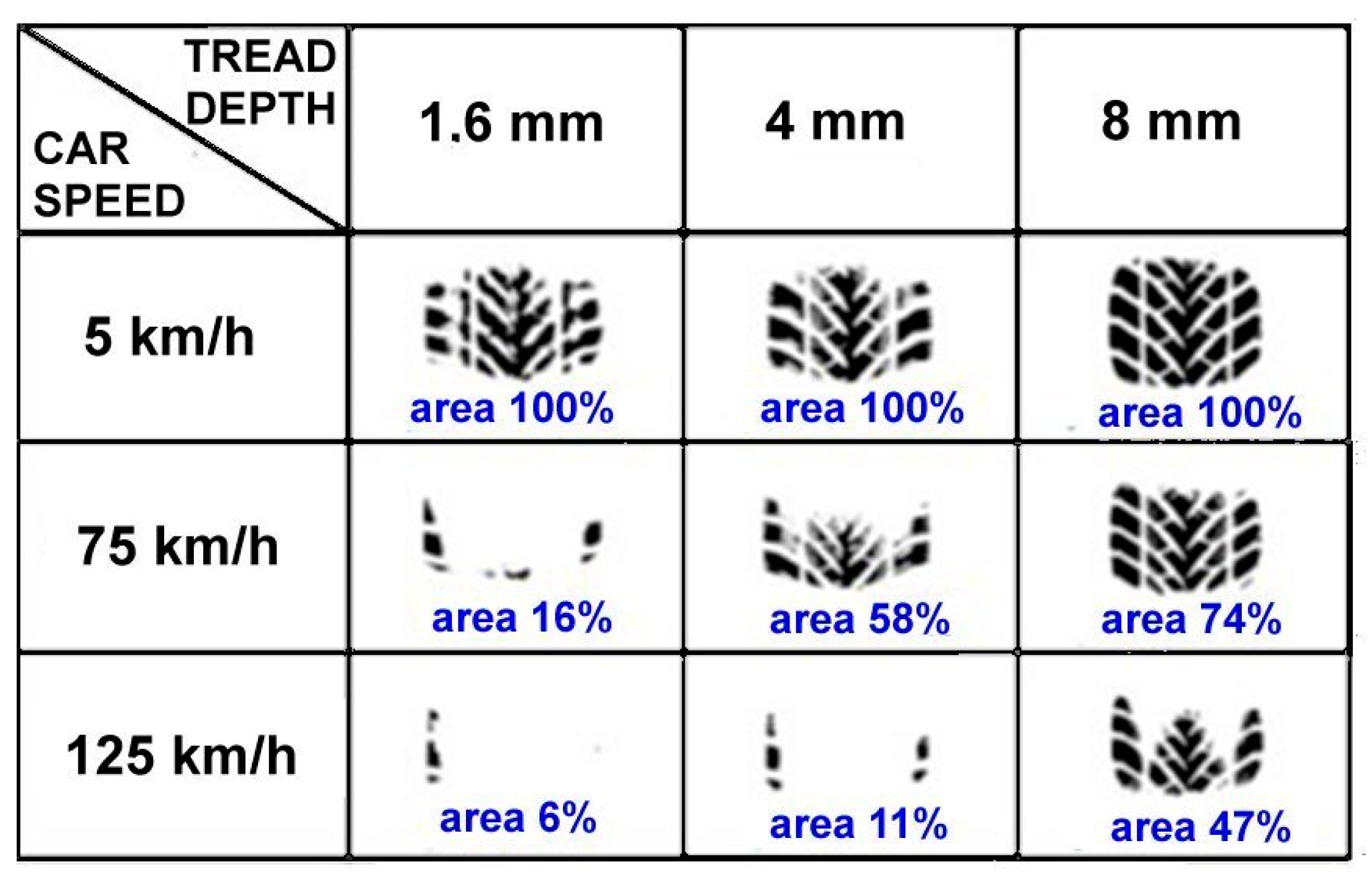
  • the quality of the compound and the condition of the tire surface;
  • quality and road surface (Table 1) [45];
  • vehicle speed;
  • conditions that are in the wheel track, mainly on the slip (slip—the rotation of the wheel is slower than the corresponding actual speed of the vehicle).
Adhesion or cohesion of the tire with the road is the most important property that affects traffic safety. Other parameters listed below are directly related to and affect adhesion. It is important for road safety that the adhesion between the wheels and the road is as high as possible. Adhesion depends on the properties of the tread rubber, relative slip speed, material, microprofile and road contamination.
Another no less important parameter of the tire (Figure 10) [43], which affects the safety of operation, is the state of wear of the tire. As the tread depth of the tires decreases during use, the braking distance of the vehicle, especially on wet roads, is considerably longer. The risk of aquaplaning (i.e., loss of vehicle contact with the road due to a water wedge between the tire and the road surface) therefore increases for tires with a small residual tread depth. From the point of view of road safety, it is therefore of the utmost importance to replace a used tire with a new one in good time, i.e., until the residual or safety depth of the groove is less than 1.6 mm.
During the formation of aquaplaning, the vehicle is completely uncontrollable, so this loss of grip is described as very dangerous. In addition, it occurs completely unexpectedly and without warning the driver. Aquaplaning is created at speeds above 80 km/h.
As indicated below, other effects include the effect of the season. The season is a factor influencing the anti-skid properties of the road surface. In summer, wet road surfaces are systematically the most slippery. This little-known and somewhat paradoxical fact follows equally from research carried out in our country and abroad. The explanation is simple: in the dry season, the road surface is abraded to an increased extent and the released particles are pushed into the softer surface when hot (especially on bituminous roads). During the longer colder period, the surface becomes somewhat brittle and the adhering particles wash away from the texture when wet. The roughness is regenerated during the winter.
The values of the coefficient of friction found during the year can be converted to the lowest summer values using approximate coefficients according to the following Table 2 [41].
The size of the adhesion is further influenced by the influence of the age of the road, the influence of the position of the tracks on the road, the influence of the road pollution, the influence of the wheel load and the influence of the tire construction. All of the above adhesion factors are reflected in the resulting vehicle deceleration value. This value is also affected by the slope of the road s. We use a positive sign for ascending, a negative sign for descending.
From relation (14) it is possible to easily calculate directly what value the achievable braking deceleration in the descent or ascent of the road will decrease or increase.
a = ( u · f + 0.01 · s ) · g
where
  • a is the achievable deceleration in m⋅s−2;
  • u is the adhesion weight ratio or braking efficiency (when all wheels of the vehicle are locked u = 1.000);
  • f is the coefficient of friction (adhesion), dimensionless value;
  • s is the slope of the road in the direction of movement of the vehicle in percent (positive incline, negative descent);
  • g is the magnitude of the gravitational acceleration g = 9.81 m⋅s−2.
It is good to realize that the adhesion weight ratio u does not reduce the effect of the longitudinal inclination, and this is therefore applied to the achievable deceleration at full size, i.e., relatively to an increased extent in vehicles where the adhesion weight ratio is less than one.
Driver’s reaction time and reaction distance are not considered in this model. The braking process is initiated at t = 0 with the first application of the brake pedal. Furthermore, for simplicity we do not take into account the other factors like gradient (gravity resistance), towing a trailer, and brake balance. Minor factors like air resistance and rolling resistance may be neglected [41,46].
Coefficient of friction, total resistive forces and grip are determined with the type and condition of the road, its temperature and how wet or damp it is, the consistency of the tire rubber, the tread pattern and also the inflation pressure [41,46]. These factors could not be simply addressed in our model but in general they can be considered with the effective value of the static friction coefficient f, or with the threshold value of the deceleration amax that must not be exceeded.
We assume an active anti-lock brake system (ABS) providing static friction, skid avoidance, which shortens the stopping distance to the minimum. For this case, the risk of skid may be considered with a greater value of the input parameter dmin [46].

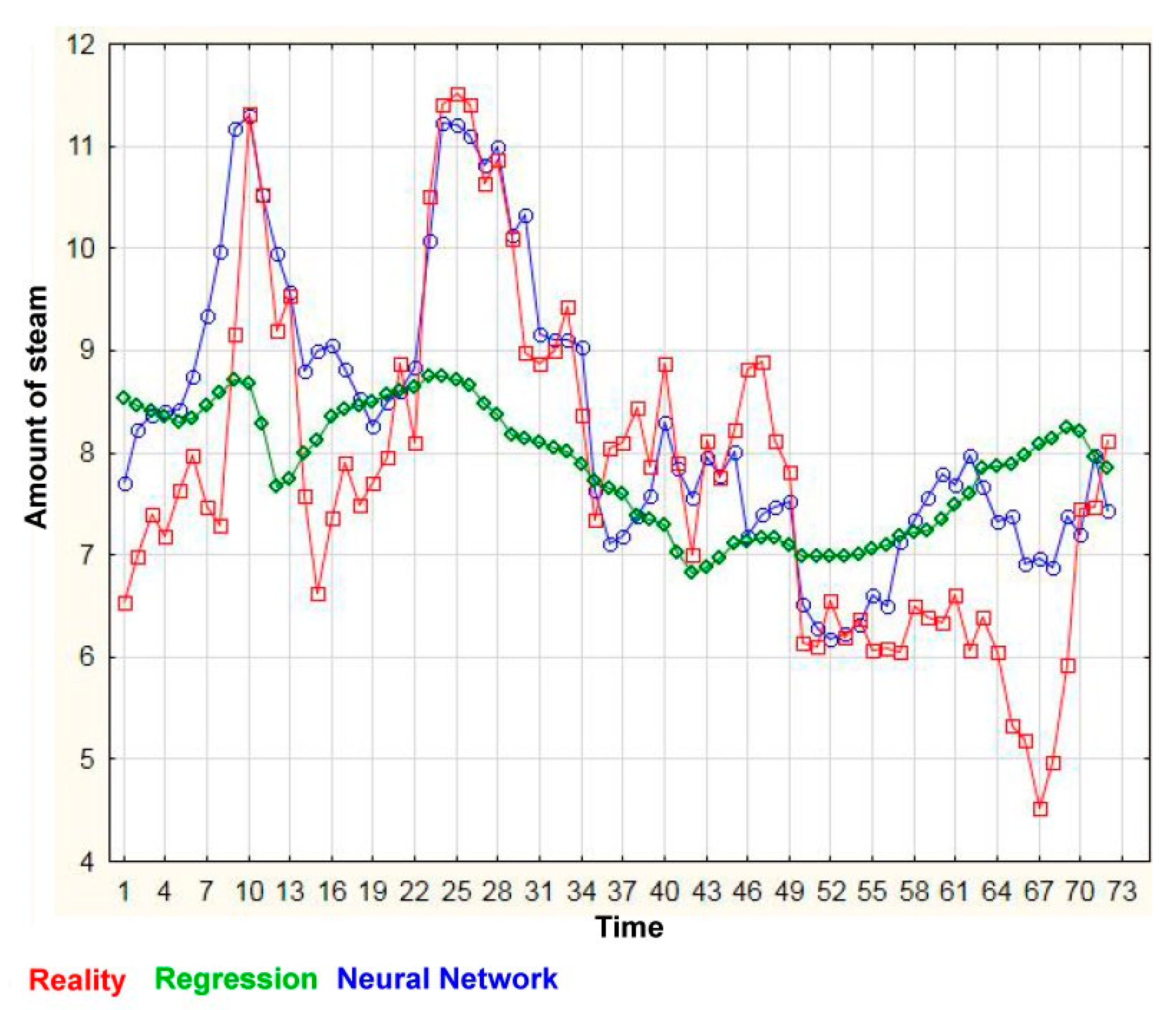
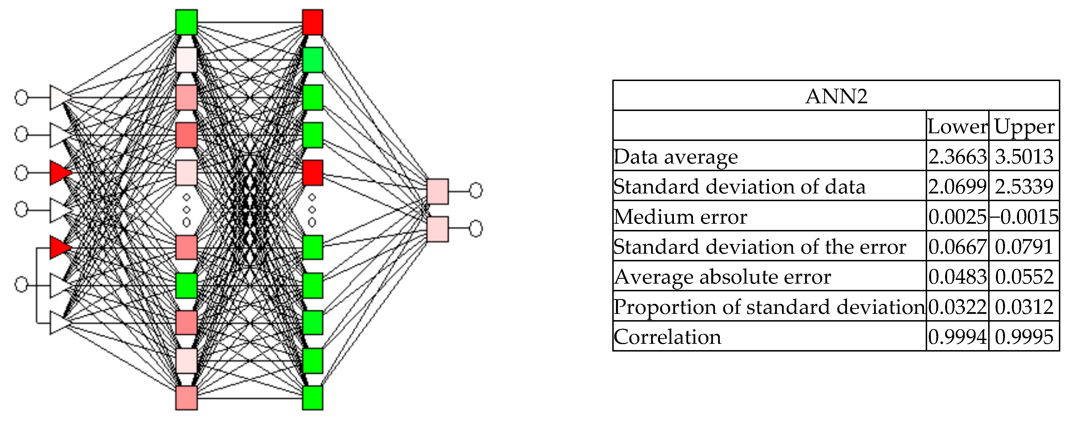
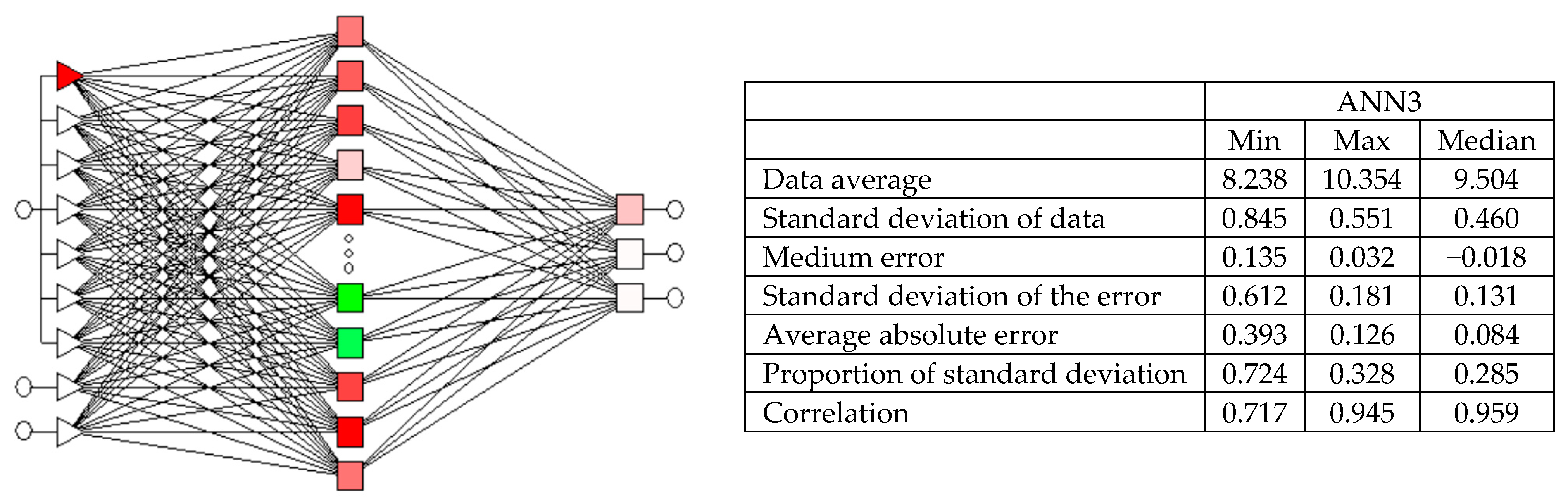
5.2. ACC Control Support Model Using Hierarchical Neural Networks

The proposed solution works with a system of three neural multilayer networks of the perceptron type. The design of the solution and individual neural networks were designed in the environment of the software STATISTICA cz, 7.1 of the company StatSoft.
STATISTICA Automated Neural Networks is one of the most advanced and powerful applications of neural network technology available on the market today. The system offers a number of unique resources and is designed not only for specialists in the field of neural networks (offering them an extraordinary range of network types and training algorithms), but also for new users of this technology (for which the Automatic Network Finder is available—steps needed to create neural networks).
If we talk about the most advanced and most powerful application, it is understood in the context that the software STATISTICA Automated Neural Networks can be included among the research simulators, which is designed for practical applications of neural networks. Unlike software types of development environments that are based on the component paradigm (Peltarion Synapse, NeuroDimension NeuroSolutions, Scientific Software Neuro Laboratory, LIONsolver, Encog, Neuroph), creating neural network models in this software system is much simpler and more comfortable, more intuitive and provides sufficient selection of neural network types for practical applications and thus the creation of a practical application is shorter in time than in software such as a development environment.
STATISTICA Automated Neural Network is an excellent application implementing neural networks, which has the following features:
  • Exceptional ease of use combined with surprising analytical performance; the automatic network finder guides the user step by step through the process of creating a group of different networks and selecting the most appropriate network with the best performance (a task that would otherwise require a lengthy “trial and error” procedure with a solid knowledge of basic theory).
  • Integrated pre and post-processing including data selection, nominal coding, scaling, normalization and replacement of missing values with interpretation for classification, regression and time series issues.
  • Advanced, highly optimized training algorithms, including the conjugate gradient method and the Broyden–Fletcher–Goldfarb–Shanno (BFGS) method; full control over all aspects that affect the behavior of the neural network, such as activation and error function or network complexity.
  • Support for combinations of networks and network architectures of virtually unlimited size organized in sets of neural networks for creating collections.
  • Comprehensive graphical and statistical feedback providing interactive exploratory analyses.
  • Full integration within the STATISTICA system; all results, graphs, reports, etc. can be further modified using the graphical and analytical tools of the STATISTICA system. It is thus possible, for example, to perform further residue analyses, create annotated summary reports, etc.
  • Full integration with STATISTICA automation tools; the user can use complete macros for all analyses, program his own analyses using a neural network in the STATISTICA Visual Basic environment or call the STATISTICA Automated Neural Network system from any COM-enabled application (Component Object Model). It can, for example, automatically perform analyses with neural networks in MS Excel tables or include neural network procedures in its own applications developed in C, C++, C#, Java, etc.
The first neural network predicts the interval value of the coefficient of adhesion (neural network output) based on three categorical variables (neural network inputs) that characterize the type of road surface (concrete, asphalt, gravel, slag, stone, ice and snow), road surface condition (in categories for individual surface types—new rough, driven, with excess tar, compacted, in bulk, compacted, broken, iceberg, oppressed and uncompressed) and the condition of the road in terms of weather (dry, wet).
The training set of neural network 1 contained 1007 patterns (examples), which were found from traffic accident analyses. This training set was randomly divided into training, validation and test sets for learning purposes in the ratio of 70%–15%–15%. As part of the learning, 25 neural networks with different structures and with different types of neural networks were tested in the STATISTICA software system. The system selected the five best according to the training performance and the achieved error parameters. Their subsequent analysis then selected the following multilayer perceptron neural network with a topology of 3:19-5-2:2 (the input layer has 3 input variables, which are categorized into 19 values—type of road surface (concrete, asphalt, gravel, slag, stone, ice and snow), condition of the road surface (in the categories for individual types of surfaces—new rough, driven, with excess tar, compacted, bulk, compacted, broken, glacial, compressed and uncompressed) and condition of the road in terms of weather (dry, wet); the hidden layer has five neurons, the output layer has two neurons providing results in a continuous form—minimum and maximum values of the coefficient of adhesion). The procedure was similar for the design of other neural networks.
The determination of the inputs to this neural network (type and condition of the road surface and the condition of the road in terms of weather conditions) is currently the subject of research by the author’s team. The research is based on the analysis of the road image, which is captured by a camera located on the front of the vehicle with subsequent classification using neural networks. At this stage, the task of determining the input values may be a weak point of the proposed system, but the research carried out by the research team is in the final phase and thus the system will soon be extended by this module for determining road type and road condition.
The topology of this neural network with the basic descriptive characteristics of the predicted quantities (data mean, standard deviation, mean error, standard deviation of the error, average absolute error, proportion of standard deviation and correlation) is shown in Figure 11.
Figure 12 is a graphical representation of the correlation between the predictions and the observed values of the interval estimate of the adhesion coefficient. The correlation for the lower limit of the adhesion coefficient is 0.9999 and for the upper limit 0.9995, which indicates an excellent learning of the neural network and thus the prediction of the interval of the adhesion coefficient with minimal error.
The resulting adhesion coefficient interval is one of the input variables of the second neural network, which predicts the deceleration interval (neural network output). This value, if it meets the deceleration limit predicted by the third neural network, would be the value that the ACC controller would work with. The prediction of the deceleration interval by the second neural network is performed depending on the interval of the adhesion coefficient, weather conditions (in categories—icing, wet drought), the size of the adhesion weight characterize the braking efficiency (technical quantity—expressing the sum of the force (gravity) action of the vehicle on the road at the points of contact with the driven wheels) and the road slope in the direction of vehicle movement.
Neural network 2 has a topology 5:7-19-16-2:2 (again a multilayer perceptron-type neural network with five input variables, four of which are continuous variables—for minimum and maximum adhesion coefficient (neural network output 1), adhesion weight characterizes braking efficiency and slope of the road in the direction of vehicle movement and 1 categorical with three categories—weather conditions in categories—icing, wet drought; the network has 2 hidden layers with 19 and 16 neurons, the output layer has 2 neurons, which represent 2 continuous variables—minimum and maximum deceleration) and descriptive characteristics are shown in Figure 13. The training set had 1100 patterns. Special sensors operating on the piezo principle or strain gauge and gyroscopic measurements can be used to obtain input values. The condition of the road in terms of weather conditions offers several variants of measurement—measuring temperature and humidity or again using the analysis of the road image.
Figure 14 is a graphical representation of the correlation between the predictions and the observed values of the upper limit of the deceleration interval estimate. The correlation for the lower deceleration limit is 0.9957 and for the upper limit 0.9966.
As indicated above, this deceleration interval is limited by the maximum deceleration value depending on the vehicle type and its parameters. This value is predicted by the proposed third neural network. Input parameters are vehicle type (in categories—minivans, small cars, lower middle class, middle class, upper middle class, upper middle class, luxury cars, sports cars and off-road vehicles), brake condition (in two limit categories—cold and warm) and vehicle loading (again in two limit categories—empty and loaded).
The maximum deceleration value (neural network output) is predicted in the form of minimum, maximum and median. The topology is again a multilayer neural network of the perceptron type with three categorical variables working with nine categories—vehicle type (in categories—minivans, small cars, lower middle class, middle class, upper middle class, upper middle class, luxury cars, sports cars and off-road vehicles), brake status (in two limit categories—cold and hot) and vehicle loading (again in two limit categories—empty and loaded), one hidden layer with 13 neurons; the output layer has three neurons, which represent three continuous variables—minimum, maximum and median maximum deceleration values). Descriptive characteristics are shown in Figure 15. The topology (again, a multilayer neural network of the perceptron type) and descriptive characteristics are shown in Figure 15.
The training set had only 24 patterns and was formed by combinations of individual categorical values; the output values were supplemented by the analysis of the conclusions from the measurements described in [32]. Measurements of input quantities could be performed, for example, by strain gauges and thermocouples.
Figure 16 is a graphical representation of the correlation between the predictions and the observed deceleration values (minimum values, maximum values, median). The correlation for the minimum deceleration value is 0.9774, for the maximum value 0.8831 and for the median deceleration 0.9055. The lower values of these correlations are given by the smaller scope of the training set.
To fulfill the required function—estimation of the deceleration parameter before the detected obstacle is from neural networks ANN1 and ANN2, whose inputs are type and condition of road surface and condition of the road in terms of weather conditions, interval value of coefficient of adhesion (output ANN1, input ANN2). In the categories—icing, wet drought, the size of the adhesive weight characterizes the effectiveness of braking and the slope of the road in the direction of vehicle movement; a hierarchical neural network is created, the output of which is an interval estimation of deceleration. This deceleration estimate will be corrected by the allowable deceleration interval, which is obtained as output from neural network 3, whose inputs are vehicle type, brake status and vehicle load—currently defined as categorical variables.
The resulting deceleration estimate value will be fed to the ACC control unit, which will trigger an action on the vehicle’s braking system. Figure 17 shows the overall arrangement of the formed neural networks with the interconnection of the ACC control unit. If we consider the values of average absolute errors of individual created and learned neural networks for different conditions and different conditions, then the average absolute error of the whole hierarchical neural network of adaptive cruise control has a value of 0.0607. The error of the method is thus 0.63%, which is acceptable. As the method is adaptive, it can be assumed that the accuracy will increase during further operation and tests.
Although the tested data come from real situations, the research team is still planning to perform real tests in various conditions and using modern sensors. Inputs to neural networks will be obtained from sensors located in the vehicle. This opens up the possibility of further research in this area. In this chapter, it has already been suggested that the team researches the possibility of using the analysis of the road image and using neural networks to determine the type and condition of the road surface and the condition of the road surface in terms of weather conditions. Another area is the application of fuzzy approaches to management support—not only in the area of categorization of variables and uncertainty of values, but especially in the area of knowledge approaches to decision support.

6. Conclusions

Today’s cars have more than ten control units that collect and evaluate data from hundreds of sensors scattered throughout the car and measure the running of various parts of the car or the state of the environment. These units include, for example, the engine control unit, ABS, ACC, air conditioning, instrument panel, airbag, automatic transmission or door.
Today, intelligent systems, including intelligent sensors, play an important role in the modern car. Emerging car technologies today work more closely with the driver and are more interactive. Very often a touch screen or human voice control is used. They are particularly important for reducing emissions, increasing safety and, above all, ensuring that the requirements for high-performance, low-fuel engines are met. In addition, these new modern systems and technologies are the way to autonomous transport, as another milestone in the development of human transport. Therefore, it is not surprising that the methods of artificial intelligence are increasingly being used in automotive systems, as evidenced by a number of research papers that have recently been published in this area.
The presented article falls into this area and presents the results achieved by the author’s team. Areas of interest are the system of adaptive cruise control and the possibility of improving this system by using neural networks. Neural networks have proven to be suitable for modeling such real systems, which are characterized by considerable complexity and great difficulty of mathematical description. They are particularly suitable for “self-learning” unstructured data with a high degree of nonlinearity and a high degree of uncertainty. They offer an interesting alternative approach to classical laborious methods of evaluating statistical data, such as regression analysis [38,39]. The neural network approach is more universal and therefore allows the capturing of much more complex relationships than these methods. All of these factors are the reasons why an adaptive cruise control system should use neural networks. Based on a simplified mathematical model of the process of braking a vehicle in front of an obstacle, a hierarchical neural network is established in the article, which estimates the deceleration parameters of the vehicle. The inputs for this unique neural network in this area are the type and condition of the road surface and the condition of the road in terms of weather conditions, interval value of adhesion coefficient, weather condition, magnitude of adhesion weight which characterize braking efficiency and road inclination. Output—the deceleration interval estimate is then corrected by another neural network, whose inputs are vehicle type, brake status and vehicle load—currently defined as categorical variables that determine the allowable deceleration interval. The subsequently corrected deceleration estimate is the input value to the ACC control unit. Input data for training sets of neural networks were obtained mainly by analyses of traffic accidents. The topology of the presented multilayer perceptron-type neural networks was determined on the basis of learning parameters of tested neural networks in the STATICTICA system with the Neural Network module, mainly according to training performance and achieved errors of the training, validation and test set. It can be stated that neural networks 1 and 2 were taught an error rate of less than 0.005, neural network 3 is less than 0.1, which is mainly due to the size of the training set and the degree of categorization of individual input variables.
An innovative factor of the article is the design of a completely original design of a hierarchical neural network, which specifies the determination of the deceleration value of the vehicle before a static or dynamic obstacle based on a number of factors and non-traditional factors that affect the braking process. It can be assumed that, in addition to the impact on driving safety, further research will also demonstrate positive effects and results in the field of optimizing fuel consumption and minimizing emissions, especially CO2. At the same time, it is another presentation of the use of artificial neural networks and modern sensors on the way to full vehicle autonomy.
Developments in the field of improving the ACC system are aimed at the use of machine vision and the so-called predictive cruise control system, which will be connected not only to other sensor systems in the car, but also to systems around the car, further deepening the car’s interaction with the external environment.

Author Contributions

Conceptualization, J.D. and P.B.; methodology, J.D. and P.B.; software, J.D., J.B., V.D.; validation, J.D., P.B., F.S., J.B.; formal analysis, J.D., P.B., F.S., J.B., V.D.; investigation, J.D.; resources, J.D.; F.S., J.B., V.D.; data curation, J.D., F.S., J.B., V.D.; writing—original draft preparation, J.D.; writing—review and editing, J.D., P.B., F.S., J.B., V.D.; visualization, J.D. and P.B.; supervision, J.D.; project administration, J.D. and P.B.; funding acquisition, J.D. All authors have read and agreed to the published version of the manuscript.

Funding

This publication was written at the ŠKODA AUTO University within the framework of the project “Use of artificial intelligence to solve economic, managerial and technical problems in the automotive industry”, from the fund of support for the long-term conceptual development of research organization provided by the Ministry of Education, Youth and Sports of the Czech Republic in the year 2021.

Institutional Review Board Statement

Not applicable.

Informed Consent Statement

Not applicable.

Conflicts of Interest

The authors declare no conflict of interest.

References

  1. Šabanovič, E.; Žuraulis, V.; Prentkovskis, O.; Skrickij, V. Identification of Road-Surface Type Using Deep Neural Networks for Friction Coefficient Estimation. Sensors 2020, 20, 612. [Google Scholar] [CrossRef] [Green Version]
  2. Andrades, I.S.; Castillo Aguilar, J.J.; García, J.M.V.; Carrillo, J.A.C.; Lozano, M.S. Low-Cost Road-Surface Classification System Based on Self-Organizing Maps. Sensors 2020, 20, 6009. [Google Scholar] [CrossRef] [PubMed]
  3. Varona, B.; Monteserin, A.; Teyseyre, A. A deep learning approach to automatic road surface monitoring and pothole detection. Pers. Ubiquit. Comput. 2020, 24, 519–534. [Google Scholar] [CrossRef]
  4. Cach, T. Udržitelná Mobilita (1 a 2). Available online: https://auto-mat.cz/19861/udrzitelna-mobilita-13-uvod-do-udrzitelne-mobility; https://auto-mat.cz/20391/udrzitelna-mobilita-23-dopravni-indukce-a-redukce (accessed on 20 December 2020).
  5. Dimil, J.; Pasad, S.; Sridhar, V.G. Intelligent Vehicle Monitoring Using Global Positioning System and Cloud Computing. Procedia Comput. Sci. 2015, 50, 440–446. [Google Scholar]
  6. Future Structure, Government Technology. Idaho, Where Self-Driving Vehicles Aren’t Currently Allowed, Forms Committee to Study Them. Available online: https://www.govtech.com/fs/Idaho-Where-Self-Driving-Vehicles-Arent-Currently-Allowed-Forms-Committee-to-Study-Them.html (accessed on 7 January 2020).
  7. Pandiyan, P.; Kiruthikamani, G.; Sarany, A.B. Intelligent Driver Monitoring and Vehicle Control System. Int. J. Sci. Res. 2017, 5, 851–853. [Google Scholar]
  8. Jones, W.D. Keeping cars from crashing. IEEE Spectr. 2001, 38, 40–45. [Google Scholar] [CrossRef]
  9. Favaró, F.; Nader, N.; Eurich, S.; Tripp, M.; Varadaraju, N. Examining accident reports involving autonomous vehicles in California. PLoS ONE 2017, 12, e0184952. [Google Scholar] [CrossRef]
  10. Vysoký, P. Asistenční systémy v automobilech. Automa 2005, 12, 2005. [Google Scholar]
  11. Dusil, T. Adaptivní Tempomat: Jak Funguje? Jaké Známe Druhy? Auto.cz. 2017. Available online: https://www.auto.cz/adaptivni-tempomat-jak-funguje-a-jake-zname-druhy-104364 (accessed on 5 January 2020).
  12. American Automobile Association, Inc. Automatic Emergency Braking with Pedestrian Detection. AAA NewsRoom. 2019. Available online: https://www.aaa.com/AAA/common/aar/files/Research-Report-Pedestrian-Detection.pdf (accessed on 12 January 2020).
  13. Jansson, J.; Johansson, J.; Gustafsson, F. Decision Making for Collision Avoidance Systems . SAE Paper 2002-01-0403. 2002. Available online: https://www.sae.org/publications/technical-papers/content/2002-01-0403/ (accessed on 12 January 2020).
  14. Wang, B.; Zhao, D.; Cheng, J. Adaptive cruise control via adaptive dynamic programming with experience replay. Soft Comput. 2019, 23, 4131–4144. [Google Scholar] [CrossRef]
  15. Wan, L.; Su, Y.; Zhang, H.; Tang, Y.; Shi, B. Neural adaptive sliding mode controller for unmanned surface vehicle steering system. Adv. Mech. Eng. 2018, 10. [Google Scholar] [CrossRef] [Green Version]
  16. Zhang, S.; Zhang, J. Neural Network Optimized Model Predictive Multi-Objective Adaptive Cruise Control. In Proceedings of the 2nd International Conference on Mechanical, Aeronautical and Automotive Engineering (ICMAA 2018) Book Series: MATEC Web of Conferences; Amir, H.F.A., Swee, S.K., Eds.; EDP Sciences: Paris, France, 2018; Volume 166, p. 01009. [Google Scholar]
  17. Lee, D.; Kwon, Y.P.; Mcmains, S.; Hedrick, J.K. Convolution Neural Network-based Lane Change Intention Prediction of Surrounding Vehicles for ACC. In Proceedings of the 2017 IEEE 20th International Conference on Intelligent Transportation Systems (ITSC), Yokohama, Japan, 16–19 October 2017. [Google Scholar]
  18. Kuyumcu, A.; Sengor, N.S. Effect of Neural Controller on Adaptive Cruise Control. In Proceedings of the Artificial Neural Networks and Machine Learning—ICANN 2016, Barcelona, Spain, 6–9 September 2016; Villa, A.E.P., Masulli, P., Rivero, A.J.P., Eds.; Lecture Notes in Computer Science; Springer: New York, NY, USA, 2016; Volume 9887, pp. 515–522. [Google Scholar]
  19. Zhao, D.; Hu, Z.; Xia, Z.; Alippi, C.; Zhu, Y.; Wang, D. Full-range adaptive cruise control based on supervised adaptive dynamic programming. Neurocomputing 2014, 125, 57–67. [Google Scholar] [CrossRef]
  20. Zhao, D.; Wang, B.; Liu, D. A supervised Actor-Critic approach for adaptive cruise control. Soft Comput. 2013, 17, 2089–2099. [Google Scholar] [CrossRef]
  21. Suresh, P.; Manivannan, P. Neural Network Based Hybrid Adaptive Controller for an Autonomously driving Car using Thin Plate Spline Radial Basis Activation Function. In Applied Mechanics and Materials; Balasubramanian, K.R., Sivapirakasam, S.P., Anand, R., Eds.; Dynamics of Machines and Mechanisms, Industrial Research; Trans Tech Publications: Zurich, Switzerland, 2014; Volume 592–594, pp. 2184–2188. [Google Scholar]
  22. Bifulco, G.; Simonelli, F.; Di Pace, R. Experiments toward an human-like Adaptive Cruise Control. In Proceedings of the 2008 IEEE Intelligent Vehicles Symposium, Eindhoven, The Netherlands, 4–6 June 2008; Volume 1–3, pp. 528–533. [Google Scholar]
  23. Huang, S.; Tan, K.; Lee, T. Autonomous cruise control using neural networks in platooning. Adv. Robot. 2005, 19, 169–189. [Google Scholar] [CrossRef]
  24. Ohno, H. Analysis and modeling of human driving behaviors using adaptive cruise control. In Proceedings of the IECON 2000: 26th Annual Conference of the IEEE Industrial Electronics Society, Nagoya, Japan, 22–28 October 2000; Volume 1–4, pp. 2803–2808. [Google Scholar]
  25. Dong, C.; Wang, H.; Li, Y.; Shi, X.; Ni, D.; Wang, W. Application of machine learning algorithms in lane-changing model for intelligent vehicles exiting to off-ramp. Transp. A Transp. Sci. 2021, 17, 124–150. [Google Scholar] [CrossRef]
  26. Mahadika, P.; Subiantoro, A.; Kusumoputro, B. Neural Network Predictive Control Approach Design for Adaptive Cruise Control. Int. J. Technol. 2020, 11, 1451–1462. [Google Scholar] [CrossRef]
  27. Kalkkuhl, J.; Hunt, K.J.; Fritz, H. FEM-based neural-network approach to nonlinear modeling with application to longitudinal vehicle dynamics control. IEEE Trans. Neural Netw. 1999, 10, 885–897. [Google Scholar] [CrossRef]
  28. Wang, J.; Zhang, L.; Zhang, D.; Li, K. An adaptive longitudinal driving assistance system based on driver characteristics. IEEE Trans. Intell. Transp. Syst. 2012, 14, 1–12. [Google Scholar] [CrossRef]
  29. Eski, I.; Yildirim, S. Neural network-based fuzzy inference system for speed control of heavy duty vehicles with electronic throttle control system. Neural Compu. Appl. 2017, 28, S907–S916. [Google Scholar] [CrossRef]
  30. Jose, D.; Nirmal, K.P.; Arfath, H.A. Fault Tolerant Adaptive Neuro-Fuzzy Based Automated Cruise Controller on FPGA. In Proceedings of the 2013 Annual IEEE India Conference (INDICON), Mumbai, India, 13–15 December 2013. [Google Scholar]
  31. Lu, P. Car cruising system incorporating ART-FNN man-machine interface in adaptation to various driving behaviors. Int. J. Comput. Appl. Technol. 1999, 12, 160–173. [Google Scholar] [CrossRef]
  32. Yan, M.; Song, J.; Zuo, L.; Yang, P. Neural Adaptive Sliding-Mode Control of a Vehicle Platoon Using Output Feedback. Energies 2017, 10, 1906. [Google Scholar]
  33. Zhao, D.; Xia, Z. Adaptive Optimal Control for the Uncertain Driving Habit Problem in Adaptive Cruise Control System. In Proceedings of the 2013 IEEE International Conference on Vehicular Electronics and Safety (ICVES), Dongguan, China, 28–30 July 2013; pp. 159–164. [Google Scholar]
  34. Lin, Y.C.; Nguyen, H.L.; Wang, C.H. Adaptive Neuro-Fuzzy Predictive Control for Design of Adaptive Cruise Control System. In Proceedings of the 2017 IEEE 14th International Conference on Networking, Sensing and Control (ICNSC 2017), Calabria, Italy, 16–18 May 2017; Fortino, G., Zhou, M.C., Lukszo, Z., Vasilakos, A.V., Basile, F., Palau, C., Liotta, A., Fanti, M.P., Guerrieri, A., Vinci, A., Eds.; IEEE: Calabria, Italy, 2017; pp. 767–772. [Google Scholar]
  35. Simonelli, F.; Bifulco, G.N.; De Martinis, V.; Punzo, V. Human-Like Adaptive Cruise Control Systems through a Learning Machine Approach. In Applications of Soft Computing: Updating the State of the Art; Avineri, E., Koppen, M., Dahal, K., Sunitiyoso, Y., Roy, R., Eds.; Springer: Berlin/Heidelberg, Germany, 2009; Volume 52, pp. 240–249. [Google Scholar]
  36. Xing, L.; He, J.; Li, Y.; Wu, Y.; Yuan, J.; Gu, X. Comparison of different models for evaluating vehicle collision risks at upstream diverging area of toll plaza. Accid. Anal. Prev. 2020, 135, 105343. [Google Scholar] [CrossRef] [PubMed]
  37. Desjardins, C.; Chaib-Draa, B. Cooperative Adaptive Cruise Control: A Reinforcement Learning Approach. IEEE Trans. Intell. Transp. Syst. 2011, 12, 1248–1260. [Google Scholar] [CrossRef]
  38. Kuman, U.A. Comparison of neural networks and regression analysis: A new insight. Expert Syst. Appl. 2005, 29, 424–430. [Google Scholar]
  39. Dreiseitla, S.; Ohno-Machado, L. Logistic regression and artificial neural network classification models: A methodology review. J. Biomed. Inform. 2002, 35, 352–359. [Google Scholar] [CrossRef] [Green Version]
  40. Pařízková, I. Modelování a simulace v oblasti odpadového hospodářství (Modelling and Simulation in the Field of Waste Management). Bachelor’s Thesis, VUT Brno, Brno, Czech Republic, 2014. [Google Scholar]
  41. Vlk, F. Elektronické systémy motorových vozidel. Soudní Inženýrství 2005, 19, 193–212. [Google Scholar]
  42. Semela, M. Analýza Silničních Nehod I; VUT Brno: Brno, Czech Republic, 2014. [Google Scholar]
  43. Toufar, P. Vliv Parametrů a Vlastností Pneumatik na Jízdní Dynamiku Vozidel; VUT Brno: Brno, Czech Republic, 2011. [Google Scholar]
  44. Vlk, F. Dynamika Motorových Vozidel; F. Vlk: Brno, Czech Republic, 2000; ISBN 80-238-5273-6. [Google Scholar]
  45. Bradáč, A. Příručka Znalce I. a II.: Analytika Silničních Nehod. PN. 60/858 A/85; Dům Techniky ČSVTS: Ostrava, Czech Republic, 1985; p. 544. [Google Scholar]
  46. How to Calculate Braking Distances. Available online: https://www.drivingtests.co.nz/resources/how-to-calculate-braking-distances/ (accessed on 23 March 2020).
Figure 1. Principle of the automatic highway.
Sustainability 13 04572 g001
Figure 2. Range and radiation diagrams of individual sensors.
Sustainability 13 04572 g002
Figure 3. Principle of adaptive cruise control.
Sustainability 13 04572 g003
Figure 4. Connection of the adaptive cruise control (ACC) system with other control units in the car.
Sustainability 13 04572 g004
Figure 5. Example of comparison of process modeling by an artificial neural network and a regression method.
Sustainability 13 04572 g005
Figure 6. Braking process with physical description. (a) braking process in terms of braking force or delay (b) braking process in terms of driving speed (c) braking process in terms of distance
Sustainability 13 04572 g006
Figure 7. System of quantities.
Sustainability 13 04572 g007
Figure 8. Forces acting on the vehicle during braking, where Bp—braking force on the front axle; Bz—braking force on the rear axle; G—gravity; Zp—front axle load; Zz—rear axle load; OfKp—rolling resistance of the front wheel; OfKz—rolling resistance of the rear wheel; Ov—air resistance; x ˙ —speed; T—center of gravity of the car; m · x ¨ —the inertia force acts at the center of gravity of the vehicle; Mrp—moment of inertia of rotating front wheels; Mrz—moment of inertia of rotating rear wheels; l—wheelbase; lp, lz, h—coordinates of the center of gravity with respect to the front and rear axles.
Sustainability 13 04572 g008
Figure 9. Introduction of non-negative descriptive parameters and quantities (as vectors).
Sustainability 13 04572 g009
Figure 10. Influence of tread depth and travel speed on the size of the contact area between the tire and the road.
Sustainability 13 04572 g010
Figure 11. Topology and descriptive characteristics of neural network 1.
Sustainability 13 04572 g011
Figure 12. Correlation of predictions and observed values of the interval estimation of the coefficient of adhesion (lower and upper limit).
Sustainability 13 04572 g012
Figure 13. Topology and descriptive characteristics of neural network 2.
Sustainability 13 04572 g013
Figure 14. Graphical representation of the correlation between the predictions and the observed values of the upper deceleration limits.
Sustainability 13 04572 g014
Figure 15. Topology and descriptive characteristics of neural network 3.
Sustainability 13 04572 g015
Figure 16. Graphical representation of the correlation of predictions and observed values of deceleration (minimum values, maximum values, median).
Sustainability 13 04572 g016aSustainability 13 04572 g016b
Figure 17. Graphical representation of the overall arrangement of neural networks and their connection with the ACC control unit.
Sustainability 13 04572 g017
Table 1. Coefficient of adhesion on different surfaces.
Road SurfaceµRoad Surfaceµ
Concretedry0.8–1.0Dirt roaddry0.4–0.6
wet0.5–0.8wet0.3–0.4
Asphaltdry0.6–0.9Grassdry0.4–0.6
wet0.3–0.8wet0.2–0.5
Pavingdry0.6–0.9Deep sand. snow 0.2–0.4
wet0.3–0.5Slippery ice0 °C0.05–0.10
Macadamdry0.6–0.8−10 °C0.08–0.15
wet0.3–0.5−20 °C0.15–0.20
Table 2. Recalculated values of the coefficient of friction.
SpringSummerAutumnWinter
MonthIII.IV.V.VI.VII.VIII.IX.X.XI.XII.I.II.
Asphalt.0.870.880.920.981.001.000.960.900.870.860.860.87
Concrete0.920.940.960.991.001.000.970.920.920.910.910.91
Asphalt = asphalt pavement cover. Concrete = cement concrete pavement cover.
Publisher’s Note: MDPI stays neutral with regard to jurisdictional claims in published maps and institutional affiliations.

