Article

A Comparative Study of Models for the Construction Duration Prediction in Highway Road Projects of India

1
Kalasalingam Academy of Research and Education, Anand Nagar, Krishnankoil 626126, Tamil Nadu, India
2
Faculty of Civil Engineering, Czestochowa University of Technology, 42201 Czestochowa, Poland
*
Authors to whom correspondence should be addressed.
Sustainability 2021, 13(8), 4552; https://doi.org/10.3390/su13084552
Submission received: 4 February 2021 / Revised: 15 March 2021 / Accepted: 30 March 2021 / Published: 20 April 2021

Abstract

:
Predicting the duration of construction projects with acceptable accuracy is a problem for contractors and researchers. Numerous researchers and tools are involved in sorting out this problem. The aim of the study is to predict the construction duration using four analytical tools as an approach. The success of construction projects in regard to time depends on various factors such as selection of contractors, consultants, cost of the projects, quality of the projects, the quantity of the projects, environmental factors, etc. Presently available commercial tools in the market are not designed as universally common and concerned. Every tool performs well in a particular situation. The prediction of India’s highway road projects duration is the biggest construction issue in the country due to various reasons. To overcome this problem, the methodology of the paper adopts various strategies to find suitable tools to predict the highway road projects’ duration, in which it classifies and analyzes the collected data. As a part of this work, the details of 363 government infrastructure projects (traditional procurement) were collected from 2000 to 2018. The present study also adopts various tools for duration prediction such as artificial neural networks (ANNs), smoothing techniques, time series analysis, and Bromilow’s time–cost (BTC) model. The results of the study recommend smoothing techniques with a constant value of 0.3, which gave the remarkable very small error of 1.2%, and its outcomes become even better when compared to other techniques.

1. Introduction

Time is considered a major factor in deciding the end of construction work; overseeing a construction project’s duration with acceptable accuracy is a problem for both contractors and researchers. A few time-related elements impact the project duration, e.g., poor execution of temporary workers, flawed structures, changing orders, customer postponement, or a ground condition [1]. Duration, expenditure, and construction quality are the three most important factors that decide the perfect completion of any construction project [2,3]. Moreover, the performance of construction time differs in various aspects, and some of the management factors have been considered in various studies [4]; some other factors also lead to delay in construction duration, such as locality, type of projects, owners, climatic condition, elevation style, number of floors, and the total floor area [5,6,7]. Among all the above factors, project cost positively correlates with project duration [8,9]. A few models for evaluating project duration have been created with numerous examinations [10,11]. Considering all the problems, a time–cost relationship is usually applied (T = KCB), and the constant K is determined using regression analysis [12,13]. Bromilow’s model is categorized further by performing both prediction models—regression analysis and artificial neural networks (ANNs)—and forecasting the time and cost of road construction projects [14]. This is used to create prediction models (exponential smoothing, ANN, regression models, and Bromilow’s time–cost (BTC) models). BTC gives fast and quantitative methods for evaluating the project duration. Considering these benefits, this research chose neural systems for demonstrating a successful construction project. In a time series analysis, an order of data is examined concerning time or different factors, and the gathered data are known as a series of time that has to accomplish a sensible mean absolute percentage error (MAPE), which correlates with the actual and predicted duration [15]. However, a higher constant range yields a quicker reaction and can create changeable values, while the lower constant range delays in predicting the values [16]. The simple exponential model has two categories of the model—the moving average and the weighted average. This technique is a highly developed and complicated method. The reason is that nine varieties of alpha values exist; thus, the selection of a suitable value is quite difficult: a low-level value of 0.1 takes the most time to react to find the duration, and a high value of 0.9 takes a very short time to react to find the duration, but in this case, accuracy is a concern. Other influencing factors, such as pricing, marketing prices, etc., cannot be used at the time of analysis. These are used only to forecast the upcoming project duration based on the previous project duration. The reason is that the upcoming project duration can be assumed based on the (past) recent project completion, which is used only to forecast the upcoming project duration. In comparison with the above models, exponential smoothing is the best technique for the completed projects [16]. This methodology results from explicit developments described by the absence of repeatable outcomes, which causes it to be more difficult to utilize the total quality management (TQM) standards [17]. The focus of this paper is to recognize and characterize the significant variables of vital administration in Small and Medium-sized Enterprises (SMEs), with a spotlight on the help area to think about its present circumstance [18]. The utilization of information and communication technology (ICT) innovations and the help of better approaches for the deduction, acting, and working in policy implementation, as well as the expanded arrangement of data and openness through different channels, are the establishment of the government [19]. In the beginning, the public authority needed to zero in on monetary change issues, yet later, it became evident that the usage of monetary change is incomprehensible without a significant change of the policy implementation, which, then again, clarifies the deferrals that happened in the use of the change [20]. The duration of the project is predicted during the planning phase itself [21]. Estimating an exact duration during planning is not accurate because many changes may happen during the construction phase [22]. The construction time has been considered one of the critical boundaries of successful projects [23]. Various public activities that begun in the most recent decade have not been finished on time. Some of them took such a long time to finish that they have gotten exhausted during development, and a significant number of their parts before development came to an end. Some had their capacities, or their proprietorship, changed during an over-long development period; in this way, they required alterations that thus prompted further expanded development and additional time and costs [24]. Although a regression model is the most widely used, we incorporated more advanced models in this paper, such as artificial neural networks, smoothing techniques, time series analysis, and Bromilow’s time–cost model. Highway construction project data were collected and analyzed to find factors affecting project final budget and duration before developing the forecasting models, research for which was based on the principle of artificial neural networks (ANNs) [25]. Highway agencies ask to estimate the time duration of projects while implementing purposes such as construction planning, contract administration, and work zone impact assessments [26]. Highway construction management’s reach is high nowadays. Time and cost are vital parameters. The project cost estimate is primarily concerned with the cost of resources needed to complete the project activities, which are employed to maintain the financial status of the project [27]. Time series is measured as one of the feasible understandings in the stochastic model. There is no limitation for ANN to follow a listing of the dataset or determine the interconnection between inputs and outputs. Likewise, ANNs are usually capable of self-acquirement and updating. Even though utilizing definite planning procedures is unavoidable, a model to anticipate or forecast time execution involves numerous analysts. This BTC model generally emphasizes certain factors to determine the project time period with the estimated final budget, and here, many surveys were conducted to evaluate this time–cost model. In exponential smoothing techniques, simple moving averages were chosen; here, more weight is given for recent data than past observations.

2. Research Methodology

2.1. Research Study

India is one of the fast-developing countries in the world in terms of infrastructure and urbanization [28]. The study obtained the infrastructure projects data from the Department of Economic Affairs, Government of India. As a part of this work, 363 finished Government infrastructure projects (traditional procurement) data were collected from 2000 to 2018. The duration prediction process details are mentioned in Figure 1. In this Problem identification is the first key point of the process. Then literature study, data collection from the authenticated source, selection of prediction tools, error comparison and predict the duration based on the minimum error.
The present study categorized these projects into two sections of new and upgraded infrastructure projects. Construction durations ranged between 78 and 4238 days. The average construction duration for the new projects was 1364.94 days and cost ranged from 40 to 536.7 crores INR (Indian Rupees). The average construction duration for upgraded projects was 934.73 days, and costs ranged from 47.99 to 639.85 crores. The following methodology was adopted in this research. Cost overrun and time constraint problems were identified, and the relevant literature was studied; then, construction project cost and time data were collected from the various sectors of the Indian Government. The expectation was that the information gathered for the forecasting technique should have similarities between data, but due to various circumstances such as cost and climatic conditions, there were deviations [29]. These kinds of data were not considered for analysis. The highly corrected data were identified for this research. Several methods are available in the market to predict the construction time based on costs, such as exponential smoothing technique, Bromilow’s time–cost model, artificial neural network, and time series analysis. In this research, four analytical models were used to find the best tools to predict the construction duration. The best prediction tools were identified using mean absolute percentage error (MAPE), mean squared error (MSE), root mean squared error (RMSE) and mean absolute deviation (MAD). The line of best fit of data points can be measured using MSE. The smaller value of RMSE indicates more accuracy of the best fit of data points. MAPE and MAD are mostly the same. The difference of actual and predicted value deviation can be calculated using MAD, and the percentage can be calculated using MAPE. The prediction error and accuracy can be measured mostly by using MAPE.
M A P E   =   100 n i n ( A P P )
M S E = 1 n 1 n ( A P ) 2
R M S E = S q . r t ( 1 n 1 n ( A P ) 2 )
M A D = 1 n 1 n . | A P |
where
n is no data available;
A is an actual value;
P is a predicted value.

2.2. Overview

Overrun of planned project time is a universal problem [30]. While reviewing the late 1960s project of Hong Kong, 70% of building projects were completed by overrunning. In another example, 70% of building projects in Saudi Arabia are also overrun 37% due to consultant concern and 84% due to poor supervision. The study of Ogunsemi [31] has opined that approximately 51% of Nigerian building projects are completed beyond schedule. The study of Czarnigowska [32] reveals that New Zealand’s overall building projects are overrun in time by 30%. Around 40% of UK building projects have also been completed beyond schedule.

2.3. Analysis

A detailed analysis of the infrastructure projects was categorized, analyzed, and results were discussed below in Table 1. Moreover, they were classified based on the status, type, government infrastructure projects duration, and time and cost overrun.

2.4. Exponential Smoothing Techniques

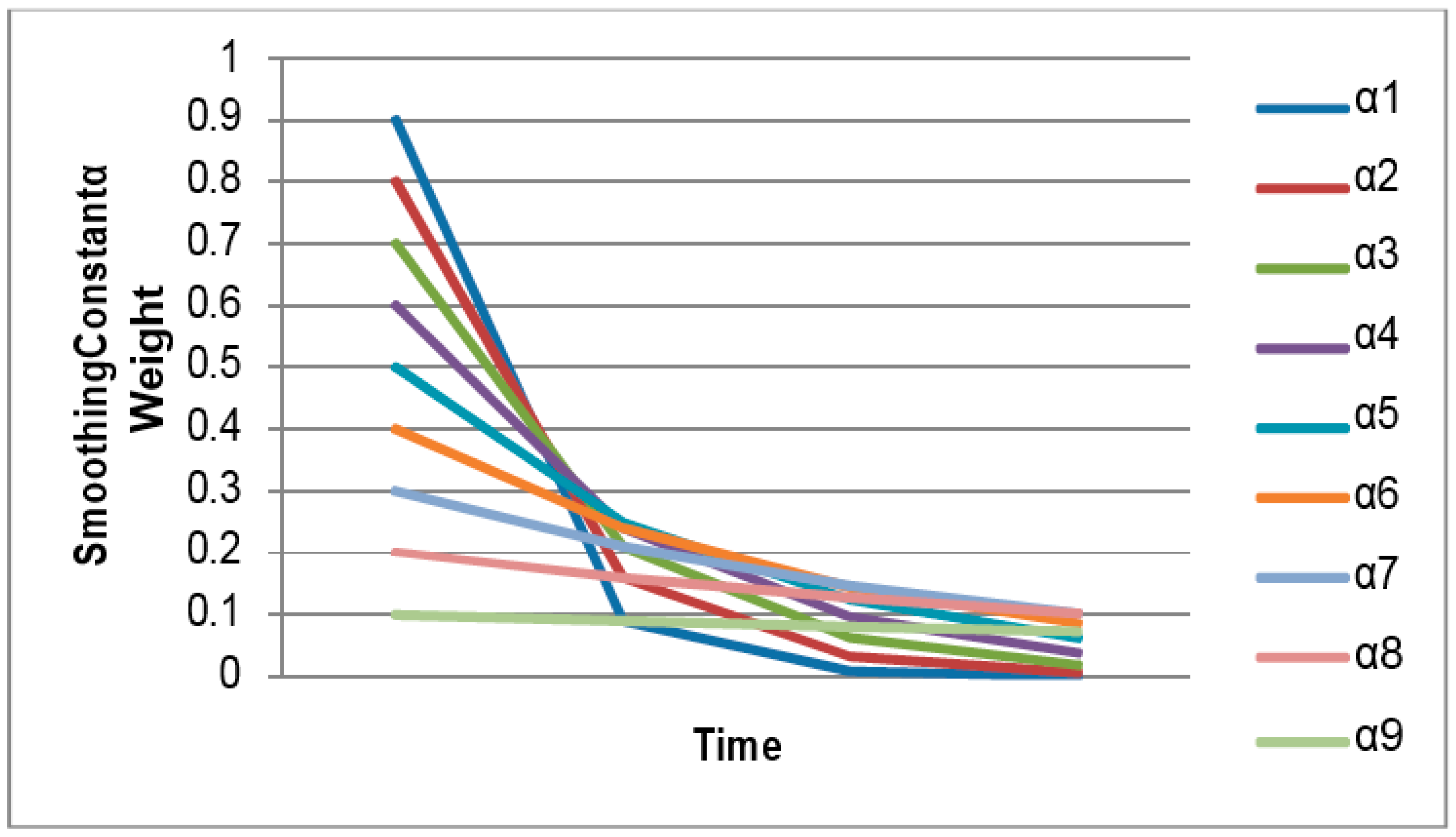
Although exponential smoothing techniques have been around since the 1950s, they only replicate a framework or model, which includes a plan designed to achieve a long-term project. However, the standard selection of the model is not established reasonably. Later, the technique was modified and extended further [33]. In this paper, a simple exponential method was used to forecast construction duration, considering that an enormous industry uses these techniques to predict time series. Here, an exact concise origin of the exponential smoothing technique is summarized. In studies, exponential smoothing techniques are completely simple predicting methods that have turned out to be significantly preferred due to their relative uniformity and great applicability in general execution by considering the patterns, regularity, and alternate features of the statistical data out of reach of human intervention [34]. In exponential smoothing techniques, the simple moving averages were chosen; more weight is given for recent data than past observations, leading to the conclusion that the earlier data affect the prediction result less than the more recent data. The exponential functions were used to assign exponentially decreasing weights over a period of time, and the constant was selected by relatively decreasing the weights of earlier data [35]. The exponential smoothing investigation apparatus utilizes the smoothing constant α, the size of which decides the amount of error previous prediction. Smoothing constant α value lies between 0 and 1, the higher value 1 (under smoothing) means that previous values have no impact on prediction, the lower value 0 (over smoothing) means that previous values have the same impact on prediction. Therefore, values ranged from 0.1 to 0.9 of α (smoothing constant) value against smoothing weight is mentioned in Table 2 and it is showing that the present idea is balanced 20–30% of error in the previous one. Here, simple exponential smoothing techniques were used because the earlier statistical data had a steady design. [36]. Figure 2 represents the graph between the time and smoothing constant. In this predicting technique, the prediction value is derived as follows:
Pt = αAt + Pt-1 (1 − α),
where Pt is the prediction time for ‘t’;
α is the smoothing constant;
At is the actual predicting time;
Pt-1 is the previous predicting time.
Smoothing constant 0.3 shows a gradual decline in line, and 0.9 shows a rapid decline in line. This graph indicates that 0.3 and 0.9 are the noted impacts in the forecasting error.

2.5. Bromilow’s Time–Cost Model

Time plays a vital role in any task, particularly in the completion of any construction project. Even though utilizing definite planning procedures is unavoidable, a model to anticipate or forecast time execution involves numerous analysts. This BTC model generally emphasizes the project period with the estimated final budget, and here, many surveys were conducted to evaluate this time–cost model [37]. Bromilow’s time–cost model is generally conceived for standard assessing contract periods in completed projects [38]. BTC provides a fast and quantitative method for evaluating project duration. It tends to be hard to obtain the data required for government projects productively, and this has subsequently directed the changes of the time–cost model’s constants “B” and “K.” The constant B depicts how the time execution is influenced by task estimate as weighed by cost [39]. There is no assurance, in any case, that the constants of the BTC method or even its frame will be the same over time [40]. Advancement in efficiency will probably speed up the process and, in this manner, will fundamentally influence the BTC model. Likewise, there is no reason to assume that the equivalent BTC model will be suitable for a wide range of tasks and strategies for obtainment [41]. Nevertheless, no other factors are considered in the BTC model other than the cost of the project. Cost and schedule execution of any project do not fundamentally vary for various works and provisions [42]. In an analysis of 363 government infrastructure projects (traditional procurement) in India, Bromilow’s has invented a new time–cost model, which proceeds to forecast the project period,
T = KCB,
where
T = duration of the project period from the date of commencement to date of completion;
C = predicted completion of the construction period;
K = duration performance is constant for 1 crore (INR) value. Generally, most research studies have used 1 million of their own country’s currency as K value [43]. Simultaneously, understanding the purpose, some of the researchers converted their country currency to USD, except a few [44]. Indian currency value, compared to a developed country, is notably low. Hence, the study considered 10 million INR (1 crore) instead of 1 million Indian currency;
B = constant determining by means of duration completion, which is altered according to the size of the project, as measured by cost.

2.6. Artificial Neural Network (ANN)

ANNs are superior to other classical statistical techniques such as the multiple regression models and the multivariate model [45]. ANNs can follow a listing of the dataset or determine the interconnection between inputs and outputs. Likewise, ANNs are usually capable of self-acquirement and updating. Considering these benefits, this research used neural systems for demonstrating a successful construction project. The rule of neural networks depends on the assumption that the interconnected arrangement of the basic process determines the complicated correlation among dependent and independent values [46]. The common artificial neural network is categorized into three layers—an input layer, a multi hidden layer, and an outer layer. These are interlinked neural networks to frame a lateral distributed system. To build up the ANN demonstration, a business programming bundle Neuro solution was chosen for its usability (worked in with Excel), speed of preparation, host of neural system structures, and incorporating the backpropagation [47]. Data of 363 government infrastructure projects (traditional procurement) were chosen as a single set for the model. Moreover, ANN predictions were determined; here, the relationship error was about 7.7%, which shows that this model is better than the regression model.

2.7. Time Series Analysis

A unique statistical approach known as time series investigation can be utilized to examine the noted time series. The significance of all the gathered data was examined, and the analytical dependence of observed data in the time series method was special and different, compared to statistical methods. Indeed, the time series analysis is the hypothesis of its correlation. As stated by Pandit [48], the numerical model for the dynamic framework is either inconsistent or varies with time and decreases in corresponding time series method of productivity to the irrelevant or explanatory data. The entire philosophy would thus be compressed as a conclusion of the corresponding model that achieves the decrease in explanatory data and afterward utilizes common statistical procedures for self-sustaining in forecasting, evaluating, and controlling. The vital concept behind the time series model is to discover a regression analysis, which shows that perception in time t, signified as Xt, as the addition of two explanatory, uncorrelated, or “symmetrical” parts, one of which is dependent on the previous data. At the same time, the other is the uncontrolled progression of the input data.

3. Results and Discussion

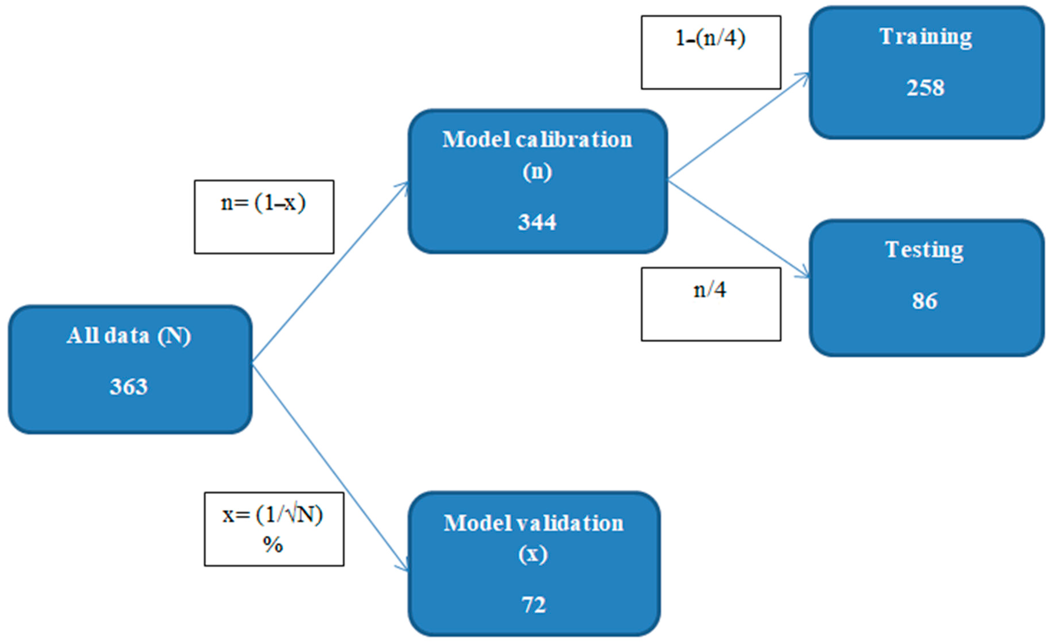
Selecting a method for data validation is the most difficult part of predictions. Akindele (1990) has opined that from the whole data, 80% of data are to be allocated for model calibration and 20% of data to be allocated for model validation. Among 363 data, 72 data were used for validation, and the rest of the data were used for calibration. Velumani [49] has suggested that reducing validate sample gives error-free results as expected. This sample concept of data validation has also been used in artificial neural networks, in which the same percentage for data validation has been applied to get the minimum error. The square root of total data (363) is 19.05, and the inverse of the square root value (1/19.05) is 0.0525. Therefore, the set of validation data is finalized as 5.25% (363 × 5.25/100 = 19.05). Approximately, 19 data were used for validation, and the balance of 344 data was used for model calibration. The allocation of data set has been represented in the Figure 3. Calibrated data and validated data have been analyzed and the values are tabulated in Table 3.
Co-efficient of determination (R2) is a value that lies between 0 and 1. Generally, the greater value of R2 is better; however, above 0.75 values are accepted for industry trends. Adjusted R2 value must be an equal or greater value of R2 model gives the best-expected result in prediction. In our model summary, 19 data R2 value is 0.824, and adjusted R2 value is 0.824. This model fits in goodness and has chances more than expected, compared to the 20% of 72 data. Error-free prediction is possible only when the validation percentage is less. Residuals statistics values are tabulated in Table 4.
This work’s R2 value is 0.824, dependent variable: time.
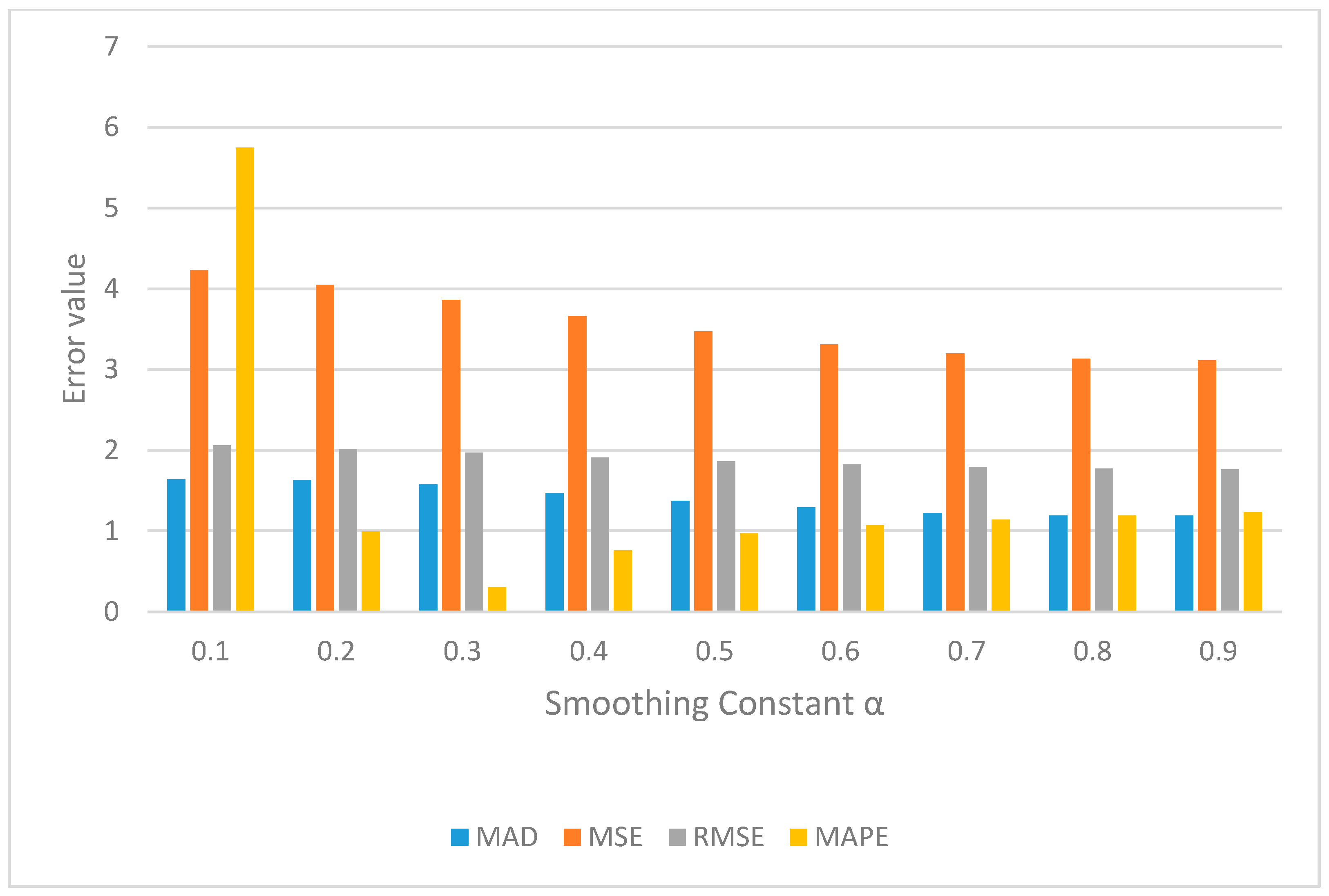
Eric Stellwagen (2018) states that a difficult moment in forecasting is finding error accuracy, because more no-of-error finding tools are available in the market, such as mean absolute deviation (MAD), mean squared error (MSE), root mean squared error (RMSE), MAD/mean ratio, geometric mean relative absolute error (GMRAE), symmetric mean absolute percentage error (SMAPE), mean absolute percentage error (MAPE), etc. MAD and MAPE are commonly used for measuring forecast error, but MAD is not efficient in high-volume data when compared to the MAPE. Therefore, in this work, MAPE was considered the measurement of error due to the high-volume level of data (363). The graph between the Error value and smoothing constant value has been shown in the Figure 4. Different forecast error values against various smoothing constant and error values against different tools are tabulated in Table 5 and Table 6 respectively.
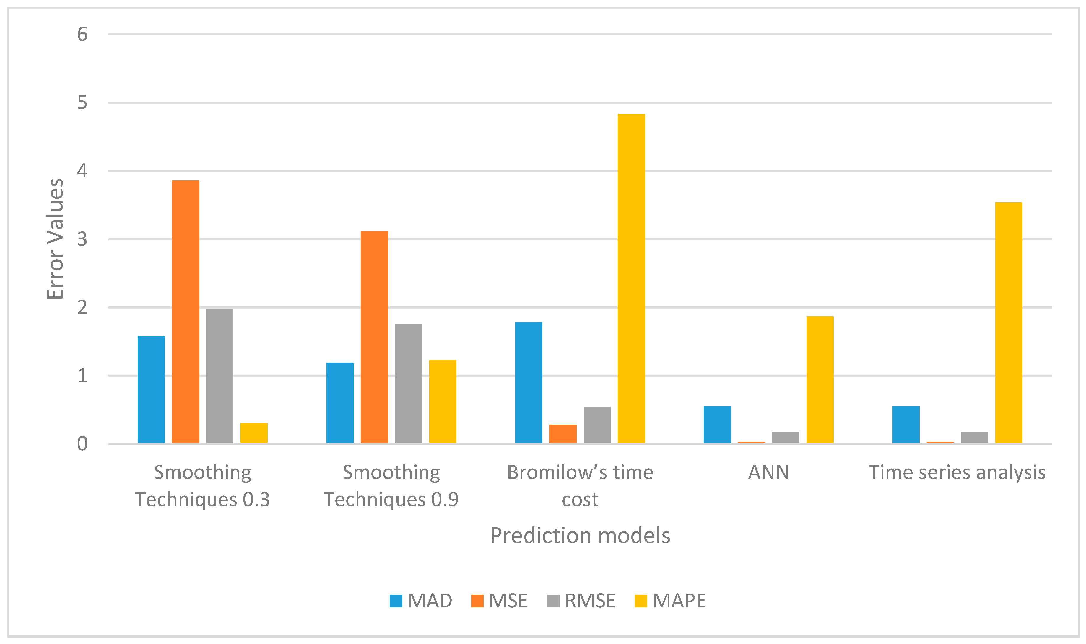
The authors have depicted the various forecast errors against different prediction techniques in Figure 5.
All log values were converted into real values to predict the actual error. Mean absolute percentage error is mentioned in Table 7 to understand the error comparative status between the different analytical tools.
The enhanced prediction process adds logical influential factors to the existing process. This process reduces the mean absolute percentage error. Despite its cost (little or substantial) and time (short or long), each project must meet a minimum of three targets such as cost, time, and execution (depends on requirements), because these three are clashing with environmental factors [47]. As per the Indian Meteorological Department (IMD) report, in earlier decades, rainfall happened gradually and moderately during monsoon seasons, but today, due to the effects of global warming, rainfall happens in dense and only very few days in India; the entire average rainfall is reached between 3 and 27 days. Therefore, construction works are affected by rainfall approximately 15 days per year. This natural factor needs to be considered to predict the duration of every project for minimizing the error. Hence, by comparing all the advanced models (smoothing techniques, Bromilow’s time–cost model, time series analysis, and ANN), we have found that a technique that gives the minimal error is the best predicting one. Here, the smoothing technique at a constant of 0.3 provides a better prediction when compared to others. The techniques adopted in the present study can be used for other projects. Here, the authors have also analyzed the methods and achieved the best methods to predict the duration of road projects.

4. Conclusions

Indian construction projects are closely associated with cost and time overrun. Therefore, a sensible approach is to reduce the time and cost overrun problem. Bromilow’s time–cost model is not efficient in Indian projects. Generally, developed countries also face this issue. At this moment, enhanced models exist that add some more influential factors and incorporate them in the existing equations, such as propagation of a time–cost model, logarithmic regression, cubic regression, exponential regression, quadratic regression, etc. The R2 value is below 0.75, which is the basic criteria to develop this kind of model, but in this work, the R2 value is 0.824. Hence, the basic model is enough to predict the same. When compared to the other prediction techniques, the artificial neural network provides competitive results with smoothing techniques constants 0.3 and 0.9; below 10% error margins are acceptable in predicting accuracy. Most of the time, influential factors do not impact construction in the long run. Sometimes, unexpected factors affect the projects in the short term; in this situation, construction time prediction effectively uses smoothing techniques with a constant of 0.3. With the help of this outcome, the same could be applied in the upcoming highway projects. Identified problems of project withdrawal, time delay completion and loss of project cost can be eliminated through the results of this research. In this research, prediction models have been evaluated, as detailed only for Indian highway road projects. More number of completed and ongoing project details are available in the data source, for which highly correlated data to cost and project duration have been segregated and analyzed in this study. The same practice may be followed to evaluate the non-correlated highway projects and other sectors of India such as state-wise housing board, railway projects, energy, infrastructure, oil and gas projects, etc. Prediction can be made by other methods as well, such as earned value management, regression analysis, etc.

Author Contributions

Conceptualization, P.V., N.V.N.N. and U.M.; Formal analysis, N.V.N.N.; Investigation, N.V.N.N. and U.M.; Methodology, P.V.; Supervision, U.M.; Validation, P.V.; Writing—original draft, Writing, P.V. and N.V.N.N.; Review & editing, U.M. All authors have read and agreed to the published version of the manuscript.

Funding

This research received no external funding.

Institutional Review Board Statement

Not applicable.

Informed Consent Statement

Not applicable.

Data Availability Statement

The data presented in this study are available on request from the corresponding author(s). The data are not publicly available due to research privacy.

Conflicts of Interest

The authors declare no conflict of interest.

References

  1. Jarkas, A.M. Predicting Contract Duration for Building Construction: Is Bromilow’s Time-Cost Model a Panacea? J. Manag. Eng. 2016, 32, 05015004. [Google Scholar] [CrossRef]
  2. Dursun, O.; Stoy, C. Determinants of construction duration for building projects in Germany. Eng. Constr. Arch. Manag. 2012, 19, 444–468. [Google Scholar] [CrossRef]
  3. Walker, D.H.T. An investigation into construction time performance. Constr. Manag. Econ. 1995, 13, 263–274. [Google Scholar] [CrossRef]
  4. Kumaraswamy, D.D. A comparative study of causes of time overruns in Hong Kong construction projects. Int. J. Proj. Manag. 1997, 15, 55–63. [Google Scholar]
  5. Skitmore, M.A. Australian project-time analysis: Statistical analysis of intertemporal trends. Constr. Manag. Econ. 2001, 19, 455–458. [Google Scholar]
  6. Le-Hoai, L.N. Estimating time performance for building construction projects in Vietnam. KSCE J. Civ. Eng. 2013, 17, 1–8. [Google Scholar] [CrossRef]
  7. Bromilow, F. Contract time performance expectations and reality. Build. Forum. 1969, 1, 70–80. [Google Scholar]
  8. Abdelhamid, T.S.; Everett, J.G. Time Series Analysis for Construction Productivity Experiments. J. Constr. Eng. Manag. 1999, 125, 87–95. [Google Scholar] [CrossRef]
  9. Al-Ghafly, M.I.-K. Important causes of delay in public utility projects in Saudi Arabia. Constr. Manag. Econ. 1999, 17, 647–655. [Google Scholar]
  10. Shr, J.F.; Chen, W.T. Functional model of cost and time for highway construction projects. J. Mar. Sci. Technol. 2006, 14, 127–138. [Google Scholar]
  11. Ammar, K. Relationship between value and duration of construction projects. Constr. Manag. Econ. 1991, 9, 383–400. [Google Scholar]
  12. Maia, A.L. Holt’s exponential smoothing and neural network models for forecasting interval-valued time series. Int. J. Forecast. 2011, 27, 740–759. [Google Scholar] [CrossRef]
  13. Love, P.T. Time-cost relationships in Australian building construction projects. J. Constr. Eng. Manag. 2005, 131, 187–194. [Google Scholar] [CrossRef]
  14. Aziz, A.M. Time Prediction for Highway Pavement Projects Using Regression Analysis. In Proceedings of the Construction Research Congress 2009, Seattle, DC, USA, 5–7 April 2009. [Google Scholar]
  15. Skitmore, M.A. Available online: https://www.tandfonline.com/doi/abs/10.1080/01446193.2001.9709621 (accessed on 29 November 2010).
  16. Brown, R.G. The fundamental theory of exponential smoothing. Opera. Res. 1961, 9, 673–685. [Google Scholar] [CrossRef]
  17. Czajkowska, A.; Kadłubek, M. Managment factors affecting quality of processes in Construction Enterprises. Pol. J. Manag. Stud. 2005, 10, 28–38. [Google Scholar]
  18. Dvorský, J.; Petráková, Z.; Ajaz, K.K.; Formánek, I.; Mikoláš, Z. Selected aspects of strategic management in the service sector. J. Tour. Serv. 2020, 20, 109–123. [Google Scholar] [CrossRef]
  19. Androniceanu, A.; Kinnunen, J.; Georgescu, I. E-Government clusters in the EU based on the Gaussian Mixture Models. Adm. Manag. Public 2020, 35, 6–20. [Google Scholar]
  20. Dong-Jun, Y.; Hae-Mi, S.; Yoo-Jun, K.; Chung-Suk, C.; Youngsuk, K. Development of an approximate construction duration prediction model during the project planning phase for general office buildings. Int. J. Civ. Eng. Manag. 2018, 24, 238–253. [Google Scholar]
  21. Yoo-Jun, K.; Dong-Jun, Y.; Young, S.K. Development of construction duration prediction model for project planning phase of mixed-use buildings. J. Asian Archit. Build. Eng. 2019, 18, 586–598. [Google Scholar]
  22. Daniela, M.; Maria, K.; Renata, B.; Marcela, S.; Katarina, K. Construction-Duration Prediction Model for Residential Buildings in Slovak Republic Based on Computer Simulation. Int. J. Appl. Eng. Res. 2017, 12, 3590–3599. [Google Scholar]
  23. Arditi, D.; Akan, G.T.; Gurdamar, S. Reasons for delays in public projects in Turkey. Constr. Manag. Econ. 1985, 3, 171–181. [Google Scholar] [CrossRef]
  24. Androniceanu, A.; Tvaronavičienė, M. Developing a holistic system for social assistance services based on effective and sustainable partnerships. Adm. Manag. Public 2019, 33, 103–118. [Google Scholar] [CrossRef]
  25. Wichan, P.; Thammasak, R.; Vannee, S. Forecasting Final Budget and Duration of Highway Construction Projects. Eng. Constr. Archit. Manag. 2009, 16, 544–557. [Google Scholar] [CrossRef]
  26. Muhammad, I.; Muhammad, B.K.; Panagiotis, C. Planning stage estimation of highway project duration on basis of project cost, project type and contract type. Int. J. Proj. Manag. 2011, 29, 78–92. [Google Scholar]
  27. Anupam, S.; Rajesh, T.; Ramtekkar, G.D. A Survey on Cost and Time management in Highway Construction Projects. Int. J. Sci. Dev. Res. (IJSDR) 2017, 2, 426–427. [Google Scholar]
  28. Jansi, R.K.; Kavitha, M.S.; Kot, S.; Hariharasudan, A. Socia-economic, hygiene and nutritional status of Indian slums: A scoping review. J. Public Health Res. Dev. 2019, 10, 128–132. [Google Scholar] [CrossRef]
  29. Vanhoucke, M. Project Management with Dynamic Scheduling, Risk Analysis and Project Control; Springer: Berlin/Heidelberg, Germany, 2012; pp. 11–35. [Google Scholar]
  30. Bromilow, F. Measurement and scheduling of construction time and cost performance in the building industry. Chart. Build. 1974, 10, 54–67. [Google Scholar]
  31. Ogunsemi, D.R. Time-cost model for building projects in Nigeria. Constr. Manag. Econ. 2007, 24, 253–258. [Google Scholar] [CrossRef]
  32. Czarnigowska, A.; Sobotka, A. Time-cost relationship for predicting construction duration. Arch. Civ. Mech. Eng. 2013, 13, 518–526. [Google Scholar] [CrossRef]
  33. Ord, J.K. Estimation and Prediction for a class of dynamic nonlinear statistical models. J. Am. Stat. Assoc. 1997, 92, 311–315. [Google Scholar] [CrossRef]
  34. Gardner. Exponential smoothing: The state of the art. J. Forecast. 1985, 22, 1–28. [Google Scholar]
  35. Taylor, J.W. Exponential smoothing with a damped multiplicative trend. Int. J. Forecast. 2003, 19, 715–725. [Google Scholar] [CrossRef] [Green Version]
  36. Maia, A.L. Available online: https://www.sciencedirect.com/science/article/abs/pii/S0169207010000506 (accessed on 2 June 2010).
  37. Homayoun, K.A.A. Project duration forecasting using earned duration management with exponential smoothing techniques. J. Manag. Eng. 2016, 33, 04016032. [Google Scholar]
  38. Ireland, V. The Role of Managerial Actions in the Cost, Time and Quality Performance of High-Rise Commercial Building Projects. Ph.D. Thesis, University of Sydney, Sydney, Australia, 1983. [Google Scholar]
  39. Bromilow, F.A. Procedures for reckoning and valuing the performance of building contracts. Chart. Build. 1976, 10, 57. [Google Scholar]
  40. Bromilow, F.E. AIQS survey of building contract time performance. Build. Econ. 1980, 19, 79–82. [Google Scholar]
  41. Chan, A.P. Time-cost relationship of public sector projects in Malaysia. Int. J. Proj. Manag. 1980, 19, 223–229. [Google Scholar] [CrossRef]
  42. Love, P.E. Influence of project type and procurement method on rework costs in building construction projects. J. Constr. Eng. Manag. 2002, 128, 18–29. [Google Scholar] [CrossRef] [Green Version]
  43. Chan, D.W.; Kumaraswamy, M.M. Modeling and predicting construction durations in Hong Kong public housing. Constr Manag. Econ. 1999, 17, 351–362. [Google Scholar] [CrossRef]
  44. Le-Hoai, L.; Young, D.L. Time-cost relationships of building construction project in Korea. Facilities 2009, 27, 549–559. [Google Scholar] [CrossRef]
  45. Elhag, T.M. Cost Modeling: Neural networks vs. regression techniques. In Proceedings of the International Conference on Construction Information Technology (INCITE), Langkawi, Malaysia, 18–21 February 2004; Construction Industry Development Board Malaysia (CIDB): Selangor, Kuala Lumpur, Malaysia, 2004. [Google Scholar]
  46. Wang, Y.R.; Gibson, G.E., Jr. A Study of Pre project Planning and Project Success Using ANN and Regression Models. Autom. Constr. 2010, 19, 341–346. [Google Scholar] [CrossRef]
  47. Zhang, Y. Forecasting Completed Cost of Highway Construction Projects Using LASSO Regularized Regression. Available online: https://ascelibrary.org/action/showCitFormats?doi=10.1061%2F%28ASCE%29CO.1943-7862.0001378 (accessed on 1 April 2021).
  48. Pandit, S.M. Time Series and System Analysis with Applications; Krieger Pub Co.: Malabar, FL, USA, 1993. [Google Scholar]
  49. Velumani, P. Predicting India’s Cement Price: A comparison of Regression analysis, Trend analysis and artificial neural network. Int. J. Civ. Eng. Technol. 2018, 9, 1907–1915. [Google Scholar]
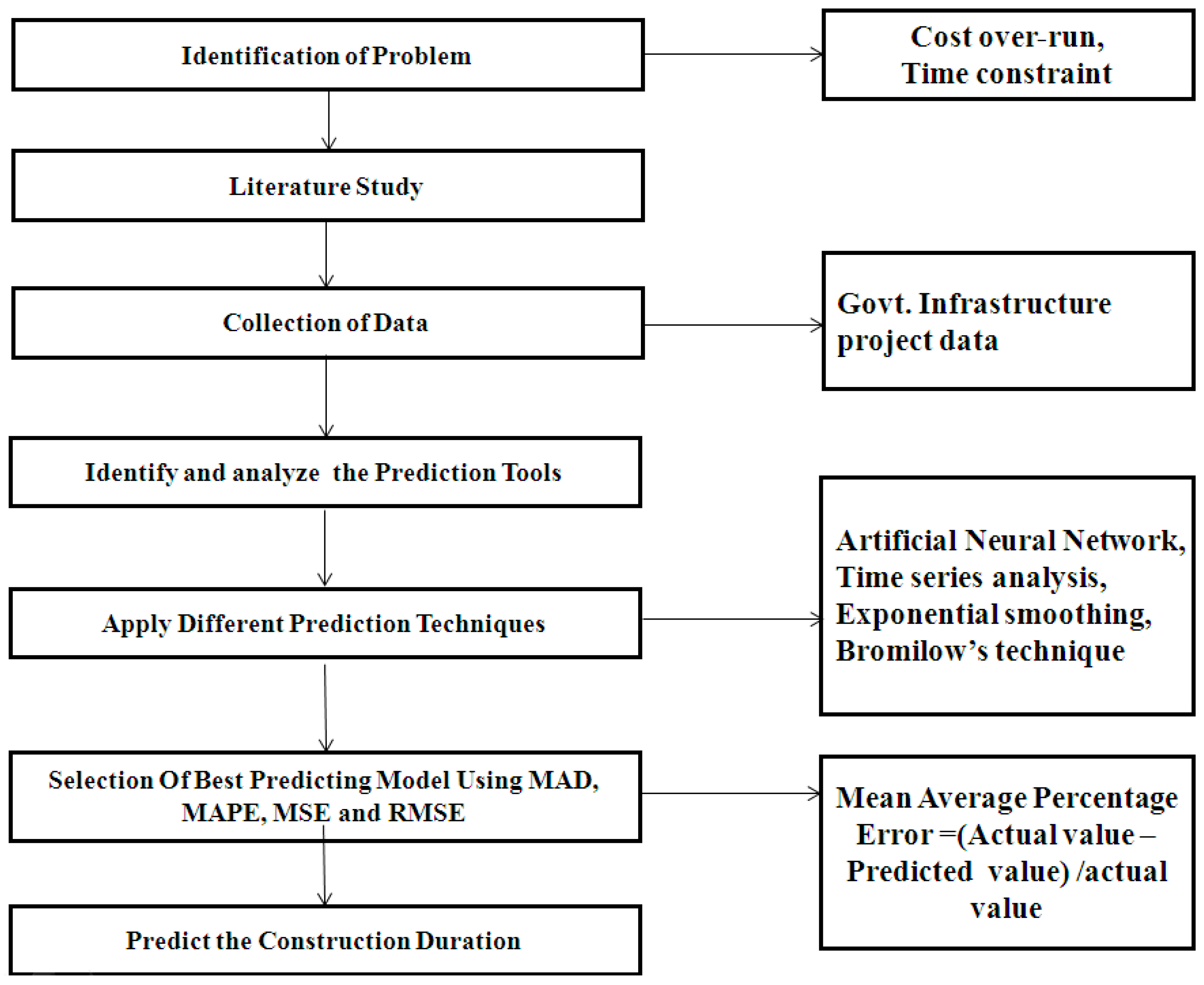
Figure 1. Conceptual framework of research.
Sustainability 13 04552 g001
Figure 2. Time vs. smoothing constant.
Sustainability 13 04552 g002
Figure 3. Allocation of data for testing, training, and validation.
Sustainability 13 04552 g003
Figure 4. Different forecast error values against various smoothing constants.
Sustainability 13 04552 g004
Figure 5. Various forecast errors against different prediction techniques.
Sustainability 13 04552 g005
Table 1. A summary of project attributes.
CategoryClassificationQuantityPercentage
Highway sectorPublic363100%
StatusCompleted (as on now)363100%
TypesNew project9125%
Up gradation27275%
GovernmentTraditional363100%
infrastructure projectProcurement
AuthorityNational level103%
(NHAI)
State level (PWD)35397%
Contract duration<1 year6718.5%
Planned1 year–2 year15342.0%
2 year–3 year9426.0%
3 year–4 year236.3%
4 year–5 year102.8%
>5 year164.4%
Time overrun>−25%205.5%
−10–−25%154.1%
0–−10%133.6%
0%10127.8%
0–10%113.0%
10–25%369.9%
>25%16746.0%
Contract cost (INR)<50328.8%
in Crore (One Crore = 10 Million)50–10023163.6%
100–2006417.6%
200–500318.5%
Note: INR–Indian Rupee.
Table 2. Smoothing constant value against smoothing weight.
Timet (1 − α)t1 (1 − α)2t2 (1 − α)3t3 (1 − α)4
Weight
α10.90.090.0090.0009
α20.80.160.0320.0064
α30.70.210.0630.0189
α40.60.240.0960.0384
α50.50.250.1250.0625
α60.40.240.1440.0864
α70.30.210.1470.1029
α80.20.160.1280.1024
α90.10.090.0810.0729
Table 3. Model summary report of 19 validated data and 72 calibrated data.
ParametersValues for 19 Validated DataValues for 72 Calibrated Data
R0.9080.851
R Square0.8240.725
Adjusted R Square0.8240.724
St. Error of the Estimate0.6910.651
F Change1603.867762.093
Sig, F Change0.0000.000
Ln K2.3132.343
K10.10510.105
B1.0030.888
Table 4. Residuals’ statistics.
MinimumMaximumMeanSt. DeviationN
Predicted Value−0.2077.6483.4271.494344
Residual−3.0001.9930.0000.690344
St. Predicted Value−2.4322.8250.0001.000344
St. Residual−4.3432.8850.0000.999344
Table 5. Different forecast error values against various smoothing constants.
Error0.10.20.30.40.50.60.70.80.9
MAD1.641.631.581.471.371.291.221.191.19
MSE4.234.053.863.663.473.313.203.133.11
RMSE2.062.011.971.911.861.821.791.771.76
MAPE5.75%0.99%0.30%0.76%0.97%1.07%1.14%1.19%1.23%
Smoothing constant α.
Table 6. Error calculated for log values.
Predicting TechniquesMADMSERMSEMAPE
Smoothing Techniques 0.31.583.861.970.30%
Smoothing Techniques 0.91.193.111.761.23%
Bromilow’s time cost1.780.280.534.83%
ANN0.550.030.171.87%
Time series analysis0.550.030.173.54%
Table 7. Mean absolute percentage error (MAPE) values for different techniques.
Prediction
Techniques
Smoothing Techniques α 0.3Smoothing
Techniques α 0.9
Bromilow’s Time Cost ModelANNTime Series Analysis
MAPE1.20%5.0221.17%7.70%15.12%
Publisher’s Note: MDPI stays neutral with regard to jurisdictional claims in published maps and institutional affiliations.