Article

Estimating Time Spent at the Waste Collection Point by A Garbage Truck with A Multiple Regression Model

Faculty of Mechanical Engineering, Wroclaw University of Science and Technology, 50-371 Wroclaw, Poland
*
Author to whom correspondence should be addressed.
Sustainability 2021, 13(8), 4272; https://doi.org/10.3390/su13084272
Submission received: 1 March 2021 / Revised: 3 April 2021 / Accepted: 6 April 2021 / Published: 12 April 2021
(This article belongs to the Section Environmental Sustainability and Applications)

Abstract

:
The planning of the garbage trucks’ routes is an essential process in waste collection companies. The main issues in garbage truck routing are determining the optimal routes, minimizing time, decreasing the costs, and reducing the pollution’s emission. In the literature, the time spent at a waste collection point (WCP) is considered as the average time, or it is not included at all. Time spent at a WCP is determined by the processes of picking up, emptying, and putting down the waste containers and the factors specific for different WCPs. Those factors impact the time spent at WCP significantly. Excluding time spent at a WCP or taking the average of that in the planning approach may lead to the inaccurate estimation of total collection time. The aim of this article is to present the multiple regression model for estimating time spent at a WCP. We analyzed the impact of the WCP factors (i.e., building type and number of containers) on the time that a garbage truck spends at it. We initially considered seven chosen factors, five categorical and two numerical. Based on this, we developed the multiple regression model based on linear regression use. Later, the proposed model was validated based on data obtained from the municipal company operating in Wroclaw city, Poland. The study confirmed that the defined factors significantly affect garbage truck’s time spent at a WCP and should be taken into account during waste collection planning processes’ performance.

1. Introduction

The waste collection process is in direct or indirect relation with sustainability aims. In Reference [1], the challenges with achieving sustainable development goals were presented. It was stated that 10 out of 17 sustainable development goals are dependent on the waste collection process. This process impacts areas related to environmental protection, public health protection, poverty reduction, and resource value. It proves the need for proper asset management in the waste collection process, which generates up to 70% of total waste management costs [2].
The municipal waste collection problems are currently a challenge in terms of economic development, population growth, and consumerism. The approaches presented in the literature focus on route planning, collection time, location of containers, costs, emission of pollutants, or energy consumption, as summarized in Reference [1].
The garbage truck routing comes to a widely analyzed vehicle-routing problem. However, in the context of waste collection, this case is more challenging to be solved. It is mainly due to a more significant number of limitations, such as the level of filling of the containers, which has to be predicted, or due to the need to take into account time windows for garbage collection (there are places where waste can be collected only during specified time windows). It leads to a higher level of complexity of such models [3].
Time is one of the most common parameters presented in the literature for waste collection optimization. In some papers, a collection time is divided into the driving time and the time spent at a waste collection point (WCP) only [4,5,6]. Time spent at a WCP can also be included more detailed by considering the time of picking up/putting down the container [7,8] and the time of inactivity (employees rest) [9], as well as the time for lunch break [2]. As a part of driving time, some authors consider the turns on the road [10,11], while others consider the time of stopping at lights [12,13].
It has been noticed that, regardless of considered parameters, there is a common feature introduced in the literature models and waste-collection-planning methods. Time spent at a WCP is generally treated as a set of processes or analyzed in detail as the time of picking up, emptying, and putting down of the containers. However, this time is usually presented as the average value, as shown in Table 1, containing selected publications dealing with waste collection modeling.
The authors of Reference [10] presented a waste-collection-route time estimation for the hauled container system. They included parameters such as the average drop-off time, average time at disposal, haul time to/from the disposal site, time spent at intersections and turns, and off-route time. Additionally, they took into account the distances covered. The time spent at a WCP was given as the average pickup time per trip. Other authors [14] proposed a model for predicting energy consumption, time requirements, and the number of garbage trucks for curbside waste collection. They specified parameters of time (average time per lift, the average time to unload, driving time, stop–go time, and time per stop based on time per lift) related to energy and distance traveled. They also considered area type, frequency of bin collection, quantity of waste, and dwelling profile. Another work [15] presented a model for predicting time and fuel consumption during waste collection. They estimated the time of collection based on the distances between the WCPs, the truck’s speed, and the time per stop. The time spent at WCP presented as time per stop was given as weighted average time per stop. In the next paper [17], which focused on mapping, the collection process’s time, average time per container, and stop time per collection point were proposed as parameters.
Regarding the estimation of the waste collection process’s costs, some authors rely on average serving time, average travel times, and time at turns [11]. The others [16] include only average service time at containers as the time parameter.
All the works mentioned above take the time spent at WCP as the average. However, the authors of Reference [13] proposed a different approach. They estimated the collection time based on population density per 100 m road distance. They considered average waiting time per stop sign and per traffic light and also pickup time. They based the pickup time on the number of containers and the number of WCPs. Additionally, in Reference [19], there can also be found some time spent at WCP estimation attempts. The authors showed two models for time per stop estimation. These models for two- and one-person crew include a number of containers at a stop, the total number of throw-away items serviced at a stop, and a number of services collected at each stop.
The literature has already emphasized that determining the time spent at WCP by garbage trucks is problematic. For this reason, the authors of Reference [9] proposed a methodology for measuring all the time types related to the waste collection process. In terms of time spent at a WCP, they emphasized that this time depends on many features, such as the container’s size, the type of vehicle, or the occurrence of overfilling of the containers. They experimentally determined the time spent at WCP for different collection systems (characterized by different types of waste, trucks, and bins, as well as bin volume and number of workers per team) but finally presented it as an average.
To sum up, the development of effective waste-collection-planning processes caused the need to include time spent at WCP by a garbage truck into waste collection models and methods. However, the conducted literature review allowed us to identify a research gap in the field of estimating time spent at WCP by a garbage truck. Currently, waste collection models include time spent at WCP as the average value, which is not a good enough representation for waste collection planning, due to too much imprecision in the predictions. Our work answers the observed research gap focusing only on one of the sub-processes of waste collection—the WCP service. This sub-process is not analyzed in the literature sufficiently (see, e.g., References [1,3,20]). Different specific factors of WCPs are not discussed enough, despite having a significant impact on time spent at WCP—to reduce or lengthen it. Papers on the subject of waste collection focus mainly on driving time. Time spent at WCP is mostly ignored or taken as the average. Following this, the article draws attention to the vital parameter of the waste collection process, which has not been a primary focus of research to date. Thus, the article aims to present a developed multiple regression model for estimating the time spent at WCP. The proposed model is based on a linear regression use, where we have linked time spent at WCP to the factors that characterize each WCP visited by a garbage truck.
Following this, the main contributions of this study are the following:
  • We have defined the main factors that influence time spend at WCP.
  • We have examined how factors may affect the time spend at WCP.
  • We have introduced a multiple regression model for predicting time spent at WCP by a garbage truck.
  • We have compared the estimation of time spent at WCP obtained from a multiple regression model with a commonly used its average value.
  • We have proposed a procedure for multiple regression modeling, which could be used in any waste collection system for garbage truck route planning performance.
  • Finally, we have validated the developed model with the use of internal and external validation methods.
Therefore, the article is structured as follows. Section 2 contains a short description of the analyzed waste collection system. Moreover, there is a description of data collection and a presentation of the proposed multiple regression model for predicting time spent at a WCP. The implementation of a multiple regression analysis follows four main steps: study design, data preparation, data analysis, and results reporting. Next, in Section 3, the results of the internal and external model validation are presented. A detailed discussion of the obtained results is provided in Section 4. Finally, in the Section 5 the whole work is summarized in the form of conclusions and the identification of further directions of our research work.

2. Materials and Methods

2.1. Waste Collection System Description

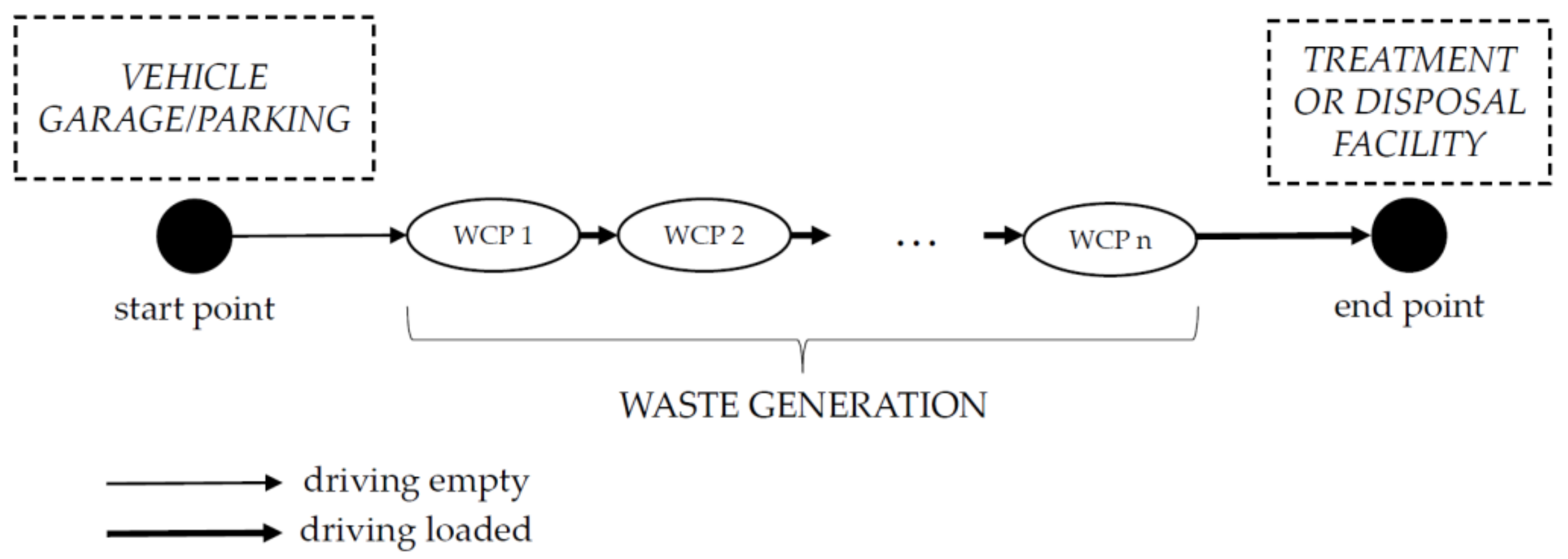
The investigated waste management system can be divided into four subsystems: waste generation system, waste collection system, waste treatment system, and waste storage and disposal system. The waste is being collected at WCPs and transported to treatment systems or directly to the storage system. The analyzed waste collection process for a single route is presented in Figure 1.
A vehicle is being weighed at the start point and then is visiting the WCPs based on a specified schedule. After visiting all the schedule points, the vehicle returns to the start point, where it is weighed again and emptied.

2.2. Data Collection

The research was conducted in the city of Wroclaw (in Poland), where the collection process is carried out according to a fixed scheme presented in Figure 1.
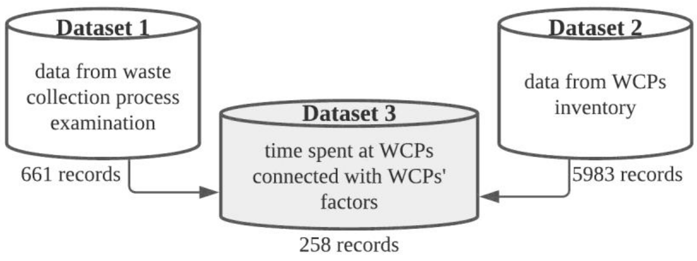
The datasets used in this paper were derived from a combination of information from two different sources (Figure 2). Dataset 1 consisted of the garbage truck drives’ data, and Dataset 2 consisted of the factors affecting the garbage truck’s stopping time at each WCP.
Data on garbage truck driving and a mixed waste collection were collected in Dataset 1. The data included information on each process’s start and end times: driving to the WCP, stopping at the WCP, and emptying the container. This database consists of 14 routes conducted by different vehicles, with different loaders, and for different WCPs located in different areas of the city. The vehicle routes are not doubled. A total of 661 individual pieces of information on the time spent at WCP are available thanks to this measurement.
Dataset 2 was based on field research consisting of collecting information on the various factors affecting the WCP collection process’s time. These factors were identified based on a literature review and information collected from garbage truck employees. The following factors were examined: WCP cover type, building type, WCP surface type, and the number of containers. These data were collected via tablets equipped with proprietary measurement applications (the survey was conducted in June–August 2020). The survey delivered the current information about the individual characteristics of 5983 WCPs. The data were collected as part of the basic research of a project supported by the National Science Centre, Poland (grant number 2019/03/X/ST8/00287), which aimed to determine the influence of the studied factors on the WCP service time.
The creation of Dataset 3 required us to link each record from Dataset 1 with the corresponding WCP from Dataset 2. Due to the lack of a key to link these databases directly, we relied on GPS coordinates. We were able to link 258 from the 661 records with their corresponding factors. Finally, we were able to consider seven factors (five categorical and two numerical) influencing time spent at a WCP by a garbage truck. To sum up, a total of eight variables were collected as Dataset 3, seven of which are factors influencing the eighth variable—time spent at WCP. The summary of the considered variables is presented in Table 2.
Time spent at WCP—This indicator represents the time required to perform all the necessary actions within the WCP. This time is counted from the moment of stopping until the vehicle leaves the WCP. Data were collected in Dataset 1.
WCP type—This is mainly divided according to the type of small architecture object, i.e., object within which the containers were placed. Three types of WCP were distinguished: freestanding containers, covered and open, covered and closed. It was verified whether the need to avoid obstacles and open the cover has a significant impact on the time spent at WCP by a garbage truck. Data were collected as part of Dataset 2.
Building type—The type of building often determines a different pickup technique for loaders. The collection process is different in single-family housing, multi-family housing, and other (e.g., stores and mixed building types). Data were collected within Dataset 2.
WCP Surface—There was considered the type of ground on which the containers are hauled as one of the factors. There are two types of surfaces: paved and unpaved. This factor seems to be much more critical when analyzed with weathering factors. However, including weathering factors would complicate the final model and make it impractical. Data were collected as part of Dataset 2.
A number of loaders—This is one of the factors considered in the literature [9,19]. Data were collected as part of Dataset 1.
Planned cleaning of WCPs—Cleaning containers may result from a random event (that type was not included in the model), but most of the work to keep WCPs clean is a planned activity. There are cleaning schedules for all the WCPs and the schedules for the specific WCPs based on the residents’ demands. In this case, the WCP service is much longer, and this factor should be taken into account during route planning. Data were collected within Dataset 1.
A number of containers—Where a container was empty or no containers were reported for collection at a given WCP (mainly single-family housing), we assumed 0. For quantities 8, 9, 11, and 12, there was insufficient representation, so they were not included in the model. Data were collected as part of Dataset 1.
Truck distance from WCP—this dataset was used to assess the fixed distance between the vehicle’s stop and the actual WCP. An example of such a situation can be gated communities. The vehicles often do not enter these communities but stop in front of the gate, and the containers are hauled from the cover to the vehicle. Data were collected as part of Dataset 1.

2.3. Multiple Regression Model

It has been verified that the use of a regression model based on only one factor is insufficient in estimating time spent at WCP by garbage truck (Table 3).
Simple regression models based on each factor separately resulted in achieving the highest R 2 = 0.584 when including only the number of containers. Therefore, multiple regression was used to predict a time spent at WCP by a garbage truck.
In linear regression, with p independent variables (predictors) X1, X2, …, Xp and a dependent variable (predicted value) Y, Equation (1) can be obtained [21]:
Y = b 0 + b 1 X 1 + b 2 X 2 +     + b p X p
In our case, we consider the variables listed in Table 2: the time spent at WCP by a garbage truck as a dependent variable and factors from Dataset 2 as independent variables.
According to Reference [22], the main stages and procedures of multiple regression analysis, presented in Figure 3, can be developed.
Based on this scheme, the following steps were performed:
  • Stage I. Study design
Due to difficulties outlined in the description of Dataset 3 development, the sample size is 258. This sample size is considered sufficient considering the sample size rule based on a number of predictors, p, proposed by Reference [22], where N > 50 + 8 * p. Additionally, it should be noticed that the used data come from different regions of the city and form different routes.
For predicting time spent at WCP by garbage truck (dependent variable), seven factors connected with WCP (independent variables) were initially chosen: WCP cover type, building type, WCP surface, number of loaders, planned cleaning, number of containers, and truck distance from WCP.
  • Stage II. Data preparation
As the first step of data preparation, data were divided into two subsets:
-
Subset 1: Two hundred measurements of the collected data for internal validation and model building;
-
Subset 2: Fifty-eight measurements of the collected data for external validation, data from two independent routes, and also from two city regions not included in Dataset 1.
Among chosen seven independent variables, five of them are categorical type. To be able to use them in the model, dummy coding [23,24] was necessary. WCP surface and planned cleaning are categorical variables with only two categories. From a variable with two categories, one variable will be created with the value 0 (absence of chosen category) or 1 (presence of chosen category). In the case of WCP type, building type, and truck distance from WCP, there are three categories in each of them. From one categorical variable with three categories, there will be created two variables with the value 0 or 1. One category must be omitted to eliminate collinearity. It should be noted at this stage that dummy coding resulted in a new, larger number of independent variables. Five categorical variables were transformed into eight independent variables (Table 4). Consequently, the initial number of seven independent variables was expanded to ten independent variables.
In the data preparation stage, there is also a need to check basic assumptions of multiple regression, which, among others, are normality, linearity, and multicollinearity.
According to the assumption of normality, residuals (the difference between observed and predicted values) should be normally distributed [25]. To check this assumption, chi^2 test was performed. It was previously stated that there are no grounds for rejecting the hypothesis about the normal distribution of residuals. Another assumption of linearity, a linear relationship between the independent and dependent variables [26], is fulfilled (non-linearity test, Lagrange multiplier = 0.735, p-value = 0.391, α = 0.05, and p-value > 0.05). Multicollinearity occurs when one of the independent variables is in a linear relationship (is strongly correlated) with one of the others [21]. Multicollinearity can be detected, for example, by examining the correlation matrix (Table 5) or with the use of variance inflation factor (VIF), with its minimum value equaling 1 and value above 10 indicating multicollinearity [27].
The coefficient of correlation values (from −0.43 to 0.23) listed in Table 5 do not indicate any significant correlation between the independent variables. This is also confirmed by the fact that every independent variable has a value of VIF slightly above 1 (from 1.125 to 1.651). Both the correlation matrix and the VIF prove that there is no multicollinearity among independent variables.
  • Stage III. Data analysis
From three main types of multiple regression (standard, sequential, and stepwise) described in Reference [28], stepwise multiple regression was used, which can only be implemented for prediction purposes [28]. In stepwise regression, there are three techniques for independent variables choosing: forward selection (adding variables one by one based on statistical criterion), backward elimination (removing variables one by one based on statistical criterion), and stepwise procedure (a combination of forward and backward). According to chosen by us backward selection, model building starts with all the independent variables, which are eliminated one by one based on a chosen criterion (for example, p-value or Mallow’s Cp [29]). The elimination process (based on the p-value in test F greater than 0.05) is presented in Table 6.
After eliminating all independent variables with a p-value greater than 0.05, the final model (Model 5) is developed. From ten independent variables inputted at the beginning, four of them were removed due to insignificance (p-value greater than 0.05). For every model R 2 and adjusted R a d j 2 , we calculated according to (2) and (3):
R 2 = i = 1 n x i x ¯ y i y ¯ i = 1 n x i x ¯ 2 i = 1 n y i y ¯ 2 2
R a d j 2 = 1 1 R 2 n 1 n p 1
where x—actual values, y—predicted values, p—number of predictors, and n—number of observations.
R 2 shows the percent of the variance in the dependent variable predicted by independent variables [28]. The more independent variables, the greater R 2 . Therefore, R a d j 2 should be used, which includes the number of predictors.
It can be noticed that the highest R a d j 2 representing predictive power was found to be 0.806 for the final model (Model 5). This model also has the lowest standard error of the estimate.
Table 7 shows the analysis results of the obtained coefficients of the final regression model.
Based on the presented coefficients, it can be stated that time spent at WCP increases as a number of containers increases. The presence of single-family or multi-family building type, truck distance from WCP 0–15 m, no planned cleaning, and a number of loaders increase causes time spent at WCP decrease. Moreover, the single-family building has more than two times greater influence on time spent at WCP decrease than multi-family building.
In accordance with the coefficients presented in Table 7, the regression model equation can be formulated as Formula (4):
t W C P =   b 0 + b 1 C n + b 2 L n + b 3 B t s + b 4 B t m + b 5 D 1 + b 6 P c n
Internal and external validation of the developed model is described in the next section (Section 3).
Results are presented in Section 3, where metrics for internal and external validation results are shown. Besides R 2 , Root Mean Square Error (RMSE) and Mean Absolute Error (MAE) were calculated with the use of Formulas (5) and (6):
R M S E =   i = 1 n x i x ¯ 2 n
M A E =   i = 1 n x i y i n
where x—actual values, y—predicted values, p—number of predictors, and n—number of observations.
3. Results

When developing a prediction model, it is necessary to consider internal and external validation. Internal validation can estimate potential overfitting [30] and internally investigate the replicability [31]. The aim of the internal validation is model testing. It shows the approximation of model performance, which will be built from the whole dataset. Among internal validation techniques, data-splitting, repeated data-splitting, jack-knife, and bootstrapping can be found [32]. We used repeated data-splitting. According to this approach, we randomly selected a portion of Subset 1 (80%) for model development and tested it on the remaining 20%. This procedure was repeated 100 times, to get different samples at each repetition, to examine different scenarios. The average results of the internal validation are presented in Table 8.
After one hundred repetitions of data-splitting, the average R 2 0.805 ( R a d j 2 0.798) of developed models was obtained. In the testing process, the average R 2 decreased to 0.764. MAE and RMSE are slightly higher. MAE (absolute difference between the actual data and the predicted data) equals 40.756 for the models’ development and 42.657 for the testing process can be considered small, taking into account the data range. RMSE indicates that the model will miss the actual values by about 43 s. Based on the obtained results, it can be stated that the model is internally validated and has a good fit. No potential overfitting has been observed.
The developed prediction model should also be externally validated before being accepted into practice [30]. For external validation purposes, a new sample of data from the same/similar population should be obtained [32]. Subset 2 (58 records) shown in the data preparation stage contains measurements from two routes and two city regions not included in Subset 1 (200 records), for internal validation. For this reason, it can be treated as a new sample from the same population. Results of the prediction model for Subset 2 are showed in Table 9.
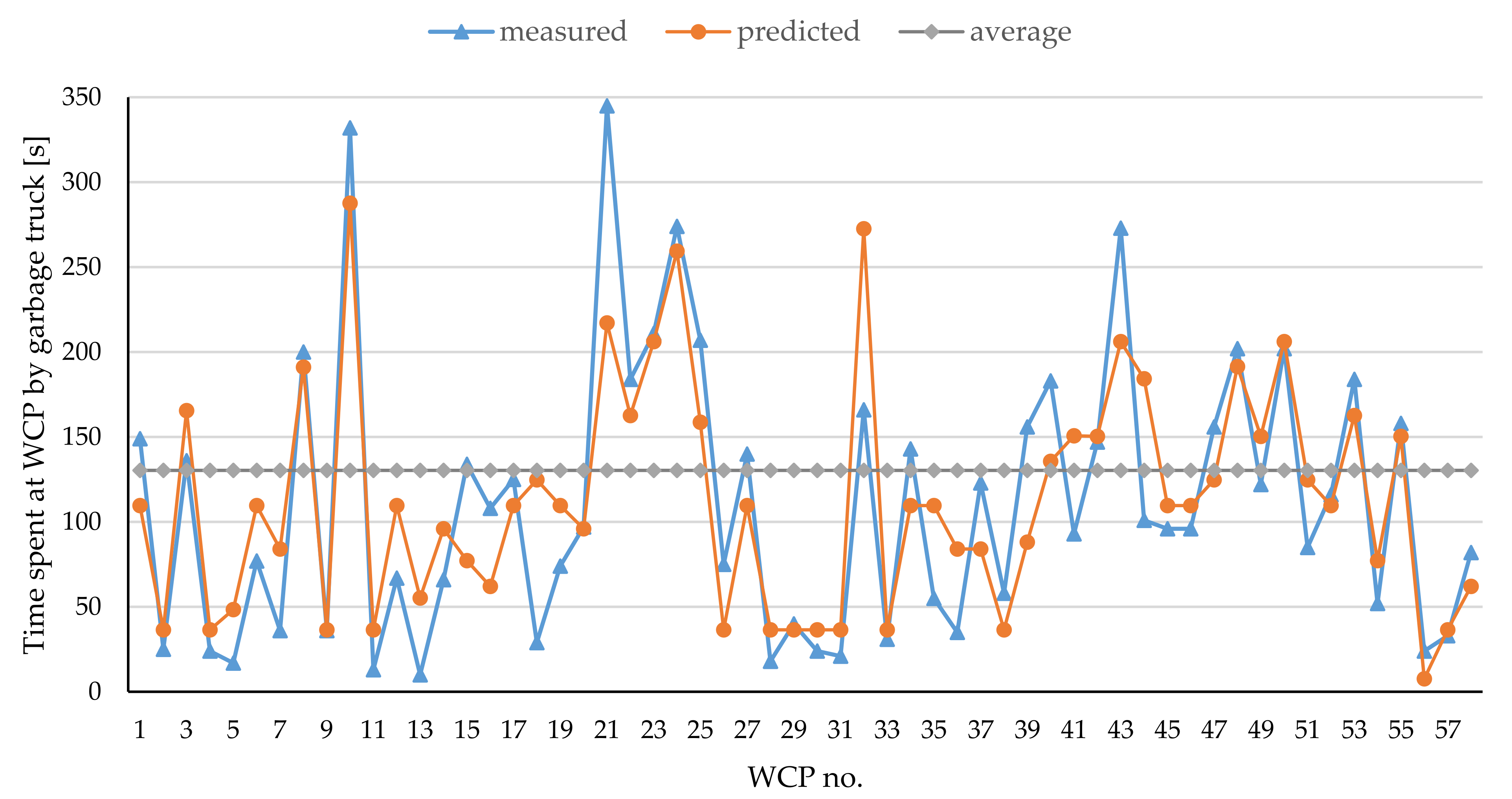
Developed prediction model with R 2 0.812 ( R a d j 2 0.806) applied to new sample performs slightly worse based on obtained lower R 2 , higher MAE and RMSE, which is expected in external validation. These results are acceptable and correspond with the results of the internal validation. They give a far more accurate representation of time spent at WCP by garbage truck than using the average value. This confirms the calculated MAE and RMSE for the commonly used average-based estimation. MAE for the average-based estimation is almost three times higher than the one obtained in external validation of our model. Looking at Figure 4 presenting measured and predicted times spent at WCP by a garbage truck, it can also be seen that the developed model gives a better estimation than using the average value.
Figure 4 clearly shows that using average time spent at WCP (the same time for each WCP) instead of its estimated values (different time for each WCP depending on its factors) results in significant under- or overestimation. Following this, taking time spent at WCP as an average value does not give a good enough representation of reality. It can be improved with the use of our model.
Time spent at WCP can take from 21% to 56% of the total waste collection time (results from Dataset 1 examination containing data from different garbage trucks and different routes). It proves that this parameter is essential in waste collection planning and should be considered with as much detail as the driving time between WCP, where, among others distances, truck speed, number of turns, stop signs, and intersections are included by different authors.

4. Discussion

The developed multiple regression model given by Formula (4) and presented in Section 2.3 was based on six independent variables. Initially, seven factors influencing time spent at WCP were considered. After dummy coding that was necessary due to the existence of categorical variables, ten independent variables were included to build the model. Based on the backward elimination approach, we eliminated four of them during the model preparation, leaving only those that were significant due to the chosen criterion (p-value). With the proposed model and the inclusion of the described variables, it is possible to achieve a better prediction of the time spent at WCP by a garbage truck than is currently done. External validation results showed that our model can predict with the error of around 47 s. However, it should be noted that it is almost three times less than with the commonly used average-based estimation.
Time spent at a WCP by a garbage truck should not be completely ignored or considered as an average value. From the sustainability point of view, it is essential to make the best possible use of the owned vehicle fleet. Significant under- or overestimation of time spent at WCP may lead to inefficient waste collection planning. WCPs can be incorrectly grouped into collection regions and improperly assigned to the garbage trucks. Following this, planned routes may turn out to be longer or shorter than expected. If the garbage truck comes back and still has resources (time, capacity, etc.) to continue the collection process, the schedule includes too many trips. More trips result in higher fuel consumption, which leads to higher emissions.
In the case of waste collection planning with time windows (some WCPs can be visited only during specified time windows), accurate prediction of time spent at a WCP by garbage truck is also crucial. If a garbage truck visits a WCP too early, it must wait, which results in ineffective use of the vehicle and workers’ time. If a garbage truck visits a WCP too late, the company will have to pay the financial penalties.
All of the abovementioned consequences of inaccurate time spent at WCP prediction can be reduced with the use of the proposed model. Better reality representation through more accurate prediction of time spent at a WCP by a garbage truck can result in more sustainable garbage-truck-fleet management.
The model can be directly applied to systems similar to the studied one, in which we see the following:
  • Diversified building type occurs,
  • Loaders work in 1 or 2 person teams,
  • Only containers are collected (we did not consider bags);
  • Waste is collected with back-loaded garbage trucks;
  • Mixed waste is collected.
If these assumptions are not met, it is necessary to perform model building as described in Section 2.
The method presented by us is characterized by more accurate predictive power than the commonly used approach based on average estimation. During predictions based on average, all variables are included without considering specific factors of WCP. For this reason, using average value can give unsatisfactory results of prediction in the case of routes with the domination of only one factor (i.e., in the case of routes with only single-family houses, there can be an overestimation of time spent at WCPs).
Our model can be valuable for waste collection planners in waste management companies. These companies currently collect data about garbage truck localization and conduct periodic WCPs inventories for their own purposes. With the proposed model’s use, waste collection can be planned more accurately, and vehicle fleet can be utilized better. Additionally, we predict that the model will find application in vehicle routing problems with time windows, where the predicted latest arrival time (affected by time spent at WCP) is of great importance. Therefore, it can be an area of interest for a wide range of experts dealing with this issue.
The most significant difficulty during model preparation was connecting information from Dataset 1 and Dataset 2. In our case, these data were collected independently. GPS localization was the only possibility for connecting. We recommend that data from garbage trucks during waste collection (Dataset 1) and data from WCPs inventory (Dataset 2) should have a common key for an easier data connection.
Finally, our model has some limitations. Data were collected during one season in the summer. Factors specific for different systems were not included. However, the procedure described in Section 2.3 is easy to follow and can be used in any collection system, including its specific features.

5. Conclusions

In the most general approach, the total time of waste collection is distinguished by the driving time (from the start point to WCP, between WCPs, and from WCP to the endpoint) and the time spent at WCP (taking the container, emptying the container, and putting the container away). The work on waste collection modeling focuses on the best possible representation of the driving time. Solutions can be found that take into account intersections, turns, traffic lights, and possible jams. However, the time spent at WCP is insufficiently analyzed. This time is often ignored or taken as the average time for WCP. Due to this, the research gap in the field of estimating time spent at WCP can be observed.
As the answer to this research gap, in this article, we have presented a multiple regression model for estimating the time spent at WCP for mixed waste. In the developed model, type of building, number of loaders, number of containers, truck distance from WCP, and planned cleaning were included as independent variables. We have obtained the adjusted coefficient of determination, R2, at the level of 0.806. Comparing predicted and measured time spent at WCP with commonly used average value showed that our approach gives far more accurate reality representation.
The presented model can be easily applied in waste management companies as part of garbage truck route planning. It was validated in the city of Wroclaw (Poland) during the summer season. For this reason, it could have some limitations, but the presented detailed procedure for multiple regression modeling ensures its reconstruction in any waste collection system. By following the steps presented in Section 2.3 and using gathered data, waste collection planners can estimate time spent at WCP more accurately.
In the future, we plan to develop a method concerning the vehicle routing problem with time windows, in which the presented model for the time spent at WCP by garbage truck estimation will be included.

Author Contributions

Conceptualization, R.G.; methodology, R.G.; software, A.D.; validation, R.G. and A.D.; formal analysis, R.G. and A.D.; investigation, R.G.; resources, R.G.; data curation, R.G.; writing—original draft preparation, A.D.; writing—review and editing, A.D.; visualization, A.D.; supervision, R.G.; project administration, R.G.; funding acquisition, R.G. All authors have read and agreed to the published version of the manuscript.

Funding

The research was partially supported by National Science Centre, Poland, grant number 2019/03/X/ST8/00287.

Institutional Review Board Statement

Not applicable.

Informed Consent Statement

Not applicable.

Data Availability Statement

The data presented in this study are available on request from the corresponding author. The data are not publicly available due to privacy.

Conflicts of Interest

The authors declare no conflict of interest.

References

  1. Hannan, M.A.; Hossain Lipu, M.S.; Akhtar, M.; Begum, R.A.; Al Mamun, M.A.; Hussain, A.; Mia, M.S.; Basri, H. Solid waste collection optimization objectives, constraints, modeling approaches, and their challenges toward achieving sustainable development goals. J. Clean. Prod. 2020, 277, 1–21. [Google Scholar] [CrossRef]
  2. Boskovic, G.; Jovicic, N.; Jovanovic, S.; Simovic, V. Calculating the costs of waste collection: A methodological proposal. Waste Manag. Res. 2016, 34, 775–783. [Google Scholar] [CrossRef] [PubMed]
  3. Han, H.; Ponce-Cueto, E. Waste collection vehicle routing problem: Literature review. Promet Traffic Traffico 2015, 27, 345–358. [Google Scholar] [CrossRef] [Green Version]
  4. Kim, B.I.; Kim, S.; Sahoo, S. Waste collection vehicle routing problem with time windows. Comput. Oper. Res. 2006, 33, 3624–3642. [Google Scholar] [CrossRef]
  5. De Bruecker, P.; Beliën, J.; De Boeck, L.; De Jaeger, S.; Demeulemeester, E. A model enhancement approach for optimizing the integrated shift scheduling and vehicle routing problem in waste collection. Eur. J. Oper. Res. 2018, 266, 278–290. [Google Scholar] [CrossRef]
  6. Chalkias, C.; Lasaridi, K. A GIS based model for the optimisation of municipal solid waste collection: The case study of Nikea, Athens, Greece. WSEAS Trans. Environ. Dev. 2009, 5, 640–650. [Google Scholar]
  7. Aringhieri, R.; Bruglieri, M.; Malucelli, F.; Nonato, M. An asymmetric vehicle routing problem arising in the collection and disposal of special waste. Electron. Notes Discret. Math. 2004, 17, 41–47. [Google Scholar] [CrossRef]
  8. Kanchanabhan, T.E.; Abbas Mohaideen, J.; Srinivasan, S.; Kalyana Sundaram, V.L. Optimum municipal solid waste collection using geographical information system (GIS) and vehicle tracking for Pallavapuram municipality. Waste Manag. Res. 2011, 29, 323–339. [Google Scholar] [CrossRef] [PubMed]
  9. Carlos, M.; Gallardo, A.; Edo-Alcón, N.; Abaso, J.R. Influence of the municipal solid waste collection system on the time spent at a collection point: A case study. Sustainability 2019, 11, 6481. [Google Scholar] [CrossRef] [Green Version]
  10. Aremu, A.S.; Mihelcic, J.R.; Fatai Sule, B. Trip time model for municipal solid waste collection applicable to developing countries. Environ. Technol. 2011, 32, 1749–1754. [Google Scholar] [CrossRef] [PubMed]
  11. Arribas, C.A.; Blazquez, C.A.; Lamas, A. Urban solid waste collection system using mathematical modelling and tools of geographic information systems. Waste Manag. Res. 2010, 28, 355–363. [Google Scholar] [CrossRef] [PubMed]
  12. Son, L.H.; Louati, A. Modeling municipal solid waste collection: A generalized vehicle routing model with multiple transfer stations, gather sites and inhomogeneous vehicles in time windows. Waste Manag. 2016, 52, 34–49. [Google Scholar] [CrossRef] [PubMed]
  13. Apaydin, O.; Gonullu, M.T. Route time estimation of solid waste collection vehicles based on population density. Glob. Nest J. 2011, 13, 162–169. [Google Scholar] [CrossRef]
  14. Edwards, J.; Othman, M.; Burn, S.; Crossin, E. Energy and time modelling of kerbside waste collection: Changes incurred when adding source separated food waste. Waste Manag. 2016, 56, 454–465. [Google Scholar] [CrossRef]
  15. Sonesson, U. Modelling of waste collection—A general approach to calculate fuel consumption and time. Waste Manag. Res. 2000, 18, 115–123. [Google Scholar] [CrossRef]
  16. Angelelli, E.; Speranza, M.G. The application of a vehicle routing model to a waste-collection problem: Two case studies. J. Oper. Res. Soc. 2002, 53, 944–952. [Google Scholar] [CrossRef]
  17. Nilssen, J.E.; Sylthe, M.; Testa, G.; Bakken, B.E. Time calculation of waste collection routes: Case study from the City of Oslo. Waste Manag. Res. 2019, 37, 667–673. [Google Scholar] [CrossRef]
  18. Ramos, T.R.P.; de Morais, C.S.; Barbosa-Póvoa, A.P. The smart waste collection routing problem: Alternative operational management approaches. Expert Syst. Appl. 2018, 103, 146–158. [Google Scholar] [CrossRef] [Green Version]
  19. Rhyner, C.R.; Schwartz, L.J.; Wenger, R.B.; Kohrell, M.G. Waste Management and Resource Recovery; CRC Press: Boca Raton, FL, USA, 1995; ISBN 9780367448936. [Google Scholar]
  20. Sulemana, A.; Donkor, E.A.; Forkuo, E.K.; Oduro-Kwarteng, S. Optimal Routing of Solid Waste Collection Trucks: A Review of Methods. J. Eng. 2018, 2018. [Google Scholar] [CrossRef] [Green Version]
  21. Oppenheim, A.J.; Cooke, W.P. Quantitative Methods for Management Decisions; McGraw-Hill Companies: New York, NY, USA, 1986; Volume 4, ISBN 9783030175535. [Google Scholar]
  22. Green, S.B. How Many Subjects Does It Take To Do A Regression Analysis? Multivar. Behav. Res. 1991, 26, 499–510. [Google Scholar] [CrossRef]
  23. Bingöl, D.; Xiyili, H.; Elevli, S.; Kılıç, E.; Çetintaş, S. Comparison of multiple regression analysis using dummy variables and a NARX network model: An example of a heavy metal adsorption process. Water Environ. J. 2018, 32, 186–196. [Google Scholar] [CrossRef]
  24. Lee, J.W.; Manorungrueangrat, P. Regression analysis with dummy variables: Innovation and firm performance in the tourism industry. In Quantitative Tourism Research in Asia. Perspectives on Asian Tourism; Rezaei, S., Ed.; Springer: Singapore, 2019; pp. 113–130. [Google Scholar] [CrossRef]
  25. Williams, M.N.; Grajales, C.A.G.; Kurkiewicz, D. Assumptions of multiple regression: Correcting two misconceptions. Pract. Assess. Res. Eval. 2013, 18, 1–14. [Google Scholar] [CrossRef]
  26. Osborne, J.W.; Waters, E. Four assumptions of multiple regression that researchers should always test. Pract. Assess. Res. Eval. 2003, 8, 2002–2003. [Google Scholar]
  27. Murray, L.; Nguyen, H.; Lee, Y.; Remmenga, M.; Smith, D.W. Variance inflation factors in regression models with dummy variables. In Proceedings of the 24th Annual Kansas State University Conference on Applied Statistics in Agriculture, Manhattan, KS, USA, 29 April–1 May 2012; pp. 161–177. [Google Scholar]
  28. Plonsky, L.; Ghanbar, H. Multiple Regression in L2 Research: A Methodological Synthesis and Guide to Interpreting R2 Values. Mod. Lang. J. 2018, 102, 713–731. [Google Scholar] [CrossRef]
  29. Desboulets, L.D.D. A review on variable selection in regression analysis. Econometrics 2018, 6, 1–27. [Google Scholar] [CrossRef] [Green Version]
  30. Shipe, M.E.; Deppen, S.A.; Farjah, F.; Grogan, E.L. Developing prediction models for clinical use using logistic regression: An overview. J. Thorac. Dis. 2019, 11, 574–584. [Google Scholar] [CrossRef]
  31. Morin, K.; Davis, J.L. Cross-validation: What is it and how is it used in regression? Commun. Stat. Theory Methods 2017, 46, 5238–5251. [Google Scholar] [CrossRef]
  32. Arboretti Giancristofaro, R.; Salmaso, L. Model Performance Analysis and Model Validation in Logistic Regression. Statistica 2007, 63, 375–396. [Google Scholar] [CrossRef]
Figure 1. The waste collection process for a single route.
Sustainability 13 04272 g001
Figure 2. Scheme of data collection.
Sustainability 13 04272 g002
Figure 3. Main stages and procedures of multiple regression.
Sustainability 13 04272 g003
Figure 4. Comparison of measured, predicted, and average-based time spent at WCP.
Sustainability 13 04272 g004
Table 1. Summary of the selected reviewed literature on waste collection modeling.
ReferenceParameters
DistanceTimeEnergyCostsTruck’s ParametersWCP Factors 1Time Spent at WCP (Model/Method)
[10]XX pickup time (average)
[9] X XXtime spent at a collection point (average)
[14]XXX XXtime per lift (average)
[12]XX XXnot included
[15]XXX XXtime per stop (weighted average)
[13]XX XXpickup time (linear regression based on no. of containers and no. of container points)
[11]XX XXXserving time (average)
[16]XX XXXservice time at containers (average)
[17]XX XXtime per container (average)
[18]XX XXXnot included
1 e.g., number of containers, amount of waste, type of waste, and area type. WCP, waste collection point.
Table 2. Summary of variables.
Variable NameVariable SymbolType of VariableCategories/Values
Time spent at WCP t W C P numerical (continuous)from 10 to 627 s
WCP cover type C t categorical (nominal)freestanding containers, covered and open, covered and close
Building type B t categorical (nominal)single-family housing, multi-family housing, other
WCP surface type S t categorical (nominal)paved, unpaved
Number of loaders L n numerical (discrete)1, 2
Planned cleaning P c categorical (nominal)no cleaning, WCP cleaning
Number of containers C n numerical (discrete)0, 1, 2, 3, 4, 5, 6, 7, 10, 13
Truck distance from WCP D categorical (nominal)0–15 m, 15–30 m, >30 m
Table 3. Summary of simple regression models results.
Considered Factor Regression   Model   R 2
Number of containers0.584
Number of loaders0.246
Planned cleaning0.215
Building type0.163
WCP cover type0.065
Truck distance from WCP0.043
WCP surface type0.002
Table 4. Categorical variables dummy coding.
Variable before CodingVariable after CodingValues
WCP cover typecovered and close C t c 0 or 1
covered and open C t o 0 or 1
Building typesingle-family B t s 0 or 1
multi-family B t m 0 or 1
Truck distance from WCP0–15 m D 1 0 or 1
above 30 m D 3 0 or 1
WCP surface typepaved S t p 0 or 1
Planned cleaningno cleaning P c n 0 or 1
Table 5. Correlation matrix (dependent variable included).
t W C P   C n L n B t s B t m D 3 D 1 C t o C t c S t p P c n
t W C P 1.0000.752−0.489−0.181−0.0850.171−0.2300.0370.267−0.027−0.442
C n 0.7521.000−0.271−0.0400.0800.009−0.0680.0530.220−0.004−0.110
L n −0.489−0.2711.0000.0710.230−0.1320.170−0.079−0.396−0.0020.140
B t s −0.181−0.0400.0711.000−0.359−0.064−0.0950.069−0.0850.1320.068
B t m −0.0850.0800.230−0.3591.000−0.0460.135−0.0190.068−0.2240.023
D 3 0.1710.009−0.132−0.064−0.0461.000−0.430−0.0440.161−0.003−0.210
D 1 −0.230−0.0680.170−0.0950.135−0.4301.000−0.037−0.125−0.0190.100
C t o 0.0370.053−0.0790.069−0.019−0.044−0.0371.000−0.140−0.1630.047
C t c 0.2670.220−0.396−0.0850.0680.161−0.125−0.1401.0000.096−0.041
S t p −0.027−0.004−0.0020.132−0.224−0.003−0.019−0.1630.0961.0000.060
P c n −0.442−0.1100.1400.0680.023−0.2100.1000.047−0.0410.0601.000
Table 6. Independent variables selection with backward elimination technique.
ModelInputted VariablesRemoved Variablesp-Value of the Removed Variable R 2 R a d j 2 Standard Error of Estimate
1 L n , C n , S t p , C t c ,   C t o , B t s , B t m , D 1 , D 3 , P c n 0.8120.80248.372
2 C t o 0.87390.8120.80348.248
3 C t o , C t c 0.88800.8120.80448.124
4 C t o , C t c , S t p 0.66560.8120.80548.022
5 C t o , C t c , S t p , D 3 0.58720.8120.80647.934
Table 7. The final model (Model 5) coefficients analysis.
b0–6SEt−Statisticp−Value
Constant317.90320.85915.245.99 × 10−35
C n 40.7332.04119.968.40 × 10−49
L n −47.5347.87−6.047.78 × 10−9
B t s −54.46711.888−4.5828.27 × 10−6
B t m −25.6337.62−3.3640.0009
D 1 −26.0269.617−2.7060.0074
P c n −175.40317.729−9.8936.30 × 10−19
Table 8. Internal validation results (average values for 100 repetitions of data-splitting).
80% Sample from Subset 1 (Model Development)20% Sample from Subset 1 (Model Testing)
R 2 0.8050.764
MAE40.75642.657
RMSE54.33556.816
Table 9. External validation results compared to model results and average-based estimation.
ModelExternal ValidationAverage-Based Estimation
R 2 0.8120.729
MAE27.95246.591128.537
RMSE41.91050.036128.543
Publisher’s Note: MDPI stays neutral with regard to jurisdictional claims in published maps and institutional affiliations.