Abstract
Hydrogen is of great significance for replacing fossil fuels and reducing carbon dioxide emissions. The application of hydrogen mixing with natural gas in gas network transportation not only improves the utilization rate of hydrogen energy, but also reduces the cost of large-scale updating household or commercial appliance. This paper investigates the necessity of a gas mixing device for adding hydrogen to existing natural gas pipelines in the industrial gas network. A three-dimensional helical static mixer model is developed to simulate the mixing behavior of the gas mixture. In addition, the model is validated with experimental results. Parametric studies are performed to investigate the effect of mixer on the mixing performance including the coefficient of variation (COV) and pressure loss. The research results show that, based on the, the optimum number of mixing units is three. The arrangement of the torsion angle of the mixing unit has a greater impact on the COV. When the torsion angle θ = 120°, the COV has a minimum value of 0.66%, and when the torsion angle θ = 60°, the COV has a maximum value of 8.54%. The distance of the mixing unit has little effect on the pressure loss of the mixed gas but has a greater impact on the COV. Consecutive arrangement of the mixing units (Case A) is the best solution. Increasing the distance of the mixing unit is not effective for the gas mixing effect. Last but not least, the gas mixer is optimized to improve the mixing performance.
1. Introduction
As one of the most promising clean energy sources, hydrogen is of great significance for replacing fossil fuel and reducing pollutants and greenhouse gas emissions [1]. Adding hydrogen to the natural gas network for the utilization of factories, gas stations, and urban communities does not only help to relieve the greenhouse gas emission, but also facilitates the market’s ability to consume hydrogen [2]. In the recent twenty years, hydrogen mixed with compressed natural gas (HCNG) has been studied for combustion of internal combustion engines [3]. Adding hydrogen to CNG as a fuel can improve engine combustion performances [4], including increasing thermal efficiency [5], decreasing combustion duration [6], extending lean burn limit, and reducing pollutants and carbon dioxide emissions [5,6,7]. So far, much research has shown that adding a certain amount of hydrogen to the natural gas can increase the combustion heat efficiency and reduce the emission of pollutants [8,9]. At present, the PREMIX code of the CHEMKIN program based on the GRI-Mech 3.0 mechanism is a commonly used numerical simulation method for studying the characteristics of the laminar premixed combustion of natural gas mixed with hydrogen [10,11]. Gimeno-Escobedo et al. [12] have explored a more computationally economical alternative to the methane-hydrogen combustion kinetic model. Based on the GRI-Mech 3.0 mechanism, the new mechanism gnf-26 of 26 substances and 143 reactions of methane-hydrogen flame has been reduced and verified. However, this mechanism is only applicable for the case with the mixing ratio of methane and hydrogen less than one: 1. De Vries et al. [13] redefines the range of blending hydrogen ratio to ensure that the mixture has a lower Wobbe Index. When the proportion of hydrogen added to the gas pipeline is 20%, the thermal comfort loss on the end users is only 4.7%, and the gas network management at this time is not complicated. Wojtowicz et al. [14] proposed that 15% hydrogen blending in natural gas can ensure the safe combustion of fuel in domestic and commercial appliances without changing the structure of gas appliances. Zhao et al. [15] proposed that the addition of hydrogen is unfeasible due to the flashback problem although the proportion of hydrogen less than 15% will not have a significant impact on the performance of the residents’ stove in domestic natural gas appliances.
For the complex gas network, there are mainly gas supply stations, gas transmission pipes, pressure regulating equipment, central gas distribution control system, solenoid valves, and residential end users [16]. Under the premise of ensuring the safe transportation of feeding hydrogen into the natural gas pipeline network, the maximum safe transport distance, inlet pressure, gas flow velocity, ambient temperature, and the geometric characteristics of the pipeline must be considered. Witkowski et al. [17] and Ogden et al. [18] believe that mixing hydrogen in natural gas pipeline requires consideration of many factors, such as market, economy, technology, and pipeline network design. Under appropriate conditions and a relatively low hydrogen concentrations (5–15%), this scheme is feasible and may require minor changes to the operation and maintenance of the pipeline network. Quarton et al. [19] studied that it is feasible to inject a certain proportion of hydrogen into the natural gas network, and the Feed in Tariffs (FITs) is €20–50/MWh. From a long-term development perspective, whether this solution is more desirable than electrification will depend on the flexibility of the gas grid linepack and the cost of expanding the power infrastructure. When hydrogen is added to natural gas pipeline, there are two main limiting factors in the mixing ratio of hydrogen, namely, supply chain conditions and end-use tolerance. In addition, the gas flow rate, velocity of hydrogen injection and the mixing device are major factors which determine the mixing performance of large-scale and long-distance transportation of hydrogen blended to natural gas network. In the case of slow laminar flow, initially the stratified mixture will be uniform at a distance of 4000 times of the nominal diameter [20]. Therefore, we believe that within a certain range, the short-distance transportation of hydrogen and natural gas mixtures may have the possibility of stratification, and there is a certain basis for the need for mixing device. However, there is rare research conducted to investigate the feasibility of hydrogen and natural gas mixture via helical static mixer (mixing device) in gas network. The mixture of hydrogen and natural gas has been homogenized in the end-user device, it can not only as a direct fuel combustion, and also provides the use of a hydrogen fuel cell vehicles [18]. In addition, the hydrogen may be separated by pressure swing adsorption (PSA) technology [21]. Therefore, the gas mixing device should be inside the gas station, a distance less than 4000 times of the nominal diameter. Conventionally, a relatively large mixing container is always used to increase the mixing contact area and time [22,23]. Although the container is more suitable for internal combustion engines with relatively small storage usage, it is not suitable for gas supply with much larger usage and fluctuations due to the size and the risk of hydrogen leakage. Basically, the application of static mixers is expected to greatly improves safety.
Static mixers have been widely used for the mixing of two-phase fluids including gas–liquid and liquid–liquid [24,25,26,27,28,29]. Zidouni et al. [24] simulated the gas–liquid flow phenomenon in the helical static mixer by CFD (Computational Fluid Dynamic) method, and analyzed the gas volume fraction, velocity, and bubble diameter on different sections. Their model can simulate the gas–liquid mixing performance of the helical static mixer including the gas phase dispersion and bubble size distribution. There are many parameters for evaluating the mixing characteristics of static mixers, including turbulent kinetic energy, shear force, and coefficient of variation (COV) [30]. In order to further improve the static mixer, some scholars have carried out further research on structural parameters and configurations. Based on the CFD simulation of RANS (Reynolds-averaged Navier–Stokes equations) method, Montante et al. [31] studied the mixing effect of two liquids with different densities and viscosities in a pipe equipped with a corrugated SMV static mixer. Compared with the simple coefficient of variation estimation, the calculation method and parameters can be easily extended to any combination of mixing elements, distributor geometry, and pipe scale, which helps to determine the best combination of geometric arrangement and physical variables. Zhuang et al. [30] studied the application of a new type of double vortex static mixer in the field of nitrogen oxide removal technology. The experimental results obtained by using particle image velocimetry (PIV) are in good agreement with their model-predicted results. Compared with other SV static mixers, the new static mixer is more efficient.
Although the gas–liquid and liquid–liquid two-phase flow in the static mixer have been studied, the analysis of the mixing effect of the gas–gas mixing in the static mixer is still rare, especially from the mixer structure to evaluate the influence of related parameters on the mixing effect. The number of mixing units, the torsion angle of the mixing units, and the distance of the mixing units are important structural parameters of the helical static mixer. It is particularly important to study its influence on the mixing process of natural gas and hydrogen in the industrial gas network system. Related research shows that the flame structure of combustion after gas premixing is stable, it is less susceptible to changes in hydrogen/air mass flow rate and equivalence ratio. When the stoichiometry is small, the pre-mixed gas combustion has better thermal performance. The use of static mixers can improve the uniformity of the gas real-time mixing and the combustion effect [32]. Furthermore, it ensures the safety of large-scale mixed hydrogen and natural gas transportation and provides a solid foundation for the sustainable development of clean energy technologies.
In this paper, a three-dimensional model is developed to simulate the mixing of natural gas and hydrogen in helical static mixer, the model is validated by comparing the model generated data with the established experimental data. Based on the model, a parametric study is performed to investigate the effects of the number of mixing units, e.g., the torsion angle of the mixing units, the distance of the mixing units on the mixing effect (coefficient of variation, COV), and pressure loss. Last but not least, we obtain the optimal structural dimensions of the helical static mixer and the operating conditions to improve the mixing effect of natural gas and hydrogen for in gas network transportation.
2. Modeling
The internal mixing units of the helical static mixer are placed vertically and staggered at 90°. The length of a single mixing unit L3 is 94 mm, the diameter D1 (D1 = D2) is 50 mm, and the thickness is 2 mm. Figure 1 takes the structure of a 7 units static mixer as an example for further introduction. The static mixer has a length of L1 which is equal to 1 m, an inner diameter of 50 mm, and a wall thickness of 1 mm. The two inlets are methane and hydrogen inlets, and the outlet is the pressure outlet condition. The horizontal distance between the hydrogen inlet and the methane inlet L2 is 200 mm, and the distance from the mixing unit is 100 mm. Figure 2 shows the cross section of the given position of the outlet of the mixing unit. Four points of the outlet section: a, b, c, d are selected to obtain the mixed gas concentration value, where the horizontal distance between a point and the center position is l1 (l1 = 6 mm), the vertical distance between b point and the center is l2 (l2 = 12 mm), the horizontal distance between point c and the center is l3 (l3 = 18 mm), and the vertical distance between point d and the center is l4 (l4 = 24 mm). According to the gas-phase component concentration values ci (i = 1, 2, 3, 4) at four points, the COV is calculated.
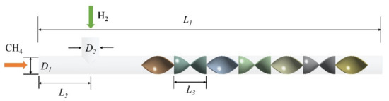
Figure 1.
Schematic diagram of helical static mixer with 7 mixing units.
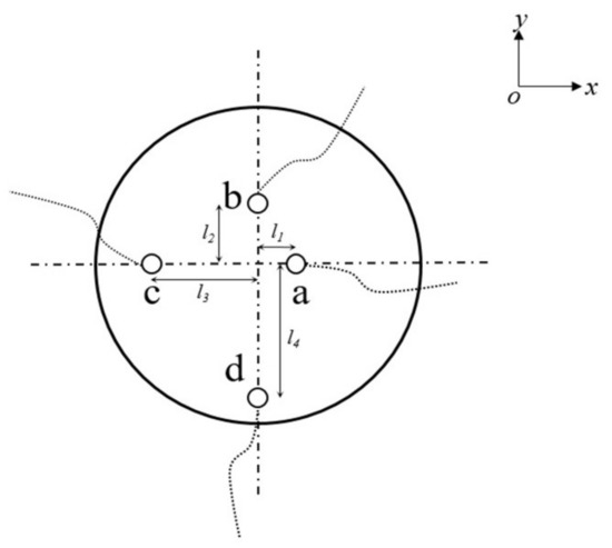
Figure 2.
Schematic diagram of points a, b, c, d at different positions of the section.
Among the main components of natural gas, the highest volume fraction of methane is 91.5% [33]. For purposes of this work, the natural gas can be simplified as pure methane. The mixture of natural gas with hydrogen can be regarded as a mixture of methane and hydrogen. Table 1 lists the physical parameters of the helical static mixer and mixed gas of different mixing units.

Table 1.
Properties parameters of helical static mixer with different units and mixed gas (25 °C, 1.01 × 10⁵ Pa).
2.1. Governing Equations
The mixed gas flow studied in this paper is in a turbulent state, and its Reynolds number calculation expression is [34]:
where
ρ—Fluid density (kg/m3)
v—Fluid velocity (m/s)
D—Equivalent diameter (m)
μ—Dynamic viscosity of fluid (Pa·s).
Adding a certain volume fraction of hydrogen to the natural gas to mix, we define the hydrogen mixing ratio XH2 of the mixed gas as
where
VCH4—The volume of methane (%)
VH2—The volume of hydrogen (%)
As one of the important parameters for evaluating the gas mixing effect, the coefficient of variation (COV) is expressed as [30]:
where
ci—The discrete phase concentration of the i-region at the outlet (mol/m3)
σ—The standard deviation
M—Total number of i regions (i = 1, 2, 3, 4)
—The volume average concentration of the discrete phase in the entire section (mol/m3).
It can be seen from Equation (3) that the COV value is between 0 and 1, and the smaller the value, the more uniform the mixing is. Based on the industrial production application, the mixing can be considered effective if the value of the coefficient of variation (COV) is less than 5% [30]. This paper studies the gas–gas mixture state. Considering the low fluid density, strong diffusivity, and small intermolecular force, the COV value is further strictly required to be below 2%.
The continuity and momentum equations are solved by a finite volume method (FVM). In the process of mixed gas flow, the mass conservation equation is satisfied:
where Sm is a user-defined generalized source term.
The momentum conservation equation is expressed as follows:
where
ρm—The mixed phase density (kg/m3)
vm—The mixed phase velocity (m/s)
P—The pressure loss at inlet and outlet of mixed phase (Pa)
g—Acceleration of gravity (m/s2)
F—Drag force between mixed phases (N)
αk—The volume fraction of the k-phase
μm—The mixed phase dynamic viscosity (Pa·s)
vdr,k—The k-phase drift velocity [m/s] (k is 1 or 2, k = 1 indicates that the first phase is methane, and k = 2 indicates that the second phase is hydrogen) [35].
2.2. Boundary Conditions
For the numerical simulation of the mixing process of methane and hydrogen, Fluent 19.0 software is used for calculation, and the pressure-based steady-state solution method is adopted. The inlets are all velocity boundary conditions, the methane inlet is set as the main phase, the hydrogen inlet is the secondary phase, and the outlet boundary is set as the pressure outlet. Due to the density of the gas is smaller, the mixed phase is turbulent flow in helical static mixer, and gravity factors have little effect on it, so it will not be considered in this paper.
The current simulation is achieved in steady-state conditions. The convection terms in the governing equations are discretized by a second order upwind scheme. The SIMPLE (Semi-Implicit Method for Pressure-Linked Equations) algorithm is used for pressure-velocity coupling. The gradients of solution variable at the cell center is determined by least square cell based. The convergence limit is set to a scaled residual lower than 10−6 for all mentioned equations.
2.3. Numerical Simulation
In order to improve the accuracy of the numerical simulation analysis of the model, taking the helical static mixer with three mixing units as an example, the cell unit sizes are 1.5 mm, 2 mm, 3 mm, 4 mm, 5 mm, and 6 mm, respectively. Table 2 records the number of cells for different cell sizes.
Table 2.
Number of cells divided by different cell sizes.
Furthermore, the volume fraction ratio of methane and hydrogen blending is selected to be 4:1 (methane accounts for 80%, hydrogen accounts for 20%), the mixing model adopts the mixture multiphase flow mixing solution model, and the turbulence model chooses the Realizable k-ε model to solve. Table 3 records the average outlet velocity and pressure loss between the inlet and outlet of helical static mixer under different cell numbers. Through the cell independence analysis, when the cell size is 2 mm, the calculation results meet the requirements.
Table 3.
The average outlet velocity and pressure loss under different cell numbers.
Given that the inlet velocity of methane is 3 m/s, the inlet velocity of hydrogen gas is calculated according to the mixing ratio of hydrogen added 20%. Table 4 records the value of hydrogen inlet velocity under 20% hydrogen ratio conditions. In addition, the settings of the number of other mixing units are the same as above.
Table 4.
Calculation parameters.
3. Experimental Setup
In order to verify the model, this paper chooses helium and air source to verify the reliability of the helical static mixer results. Note that the helium and air, which are safer and more accessible than the hydrogen and natural gas, are chosen to validate the model due to the similar densities. Figure 3 presents a schematic diagram of the experimental test system device. Helium (the volume fraction is 20%) and air (the volume fraction is 80%) flows in a helical static mixer, and then the data is recorded by a flow meter and a pressure gauge and the final mixed gas is discharged into the atmosphere. SY-9321 mass flow meter is selected as the flow meter in the experimental device, and the instrument measurement accuracy is ±1.5% F.S. The LCD digital pressure gauge is HG-808XB high-precision pressure gauge, with a measurement accuracy of ±1% F.S. The helical static mixer uses SK-68650 static mixer with an inner diameter of 50 mm and a maximum pressure of 1 Mpa. Table 5 presents a detailed list of experimental system instruments. The gas flow tube has a diameter of 12 mm, and each instrument is connected by a tracheal quick plug interface.
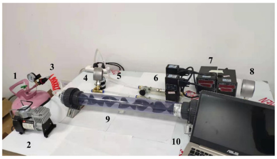
Figure 3.
Schematic diagram of experimental test system device.1—Helium tank, 2—Air pump, 3—Pressure reducing valve, 4—Pressure gauge, 5—Rubber pipe, 6—Flow meter, 7—Flow digital display instrument, 8—Pressure gauge, 9—Helical static mixer, 10—Computer.
Table 5.
List of instruments of the test system.
Figure 4 shows a schematic diagram of the gas mixing experiment for verifying the helical static mixer model. During the experiment, we firstly open the air pump valve and keep the tube ventilated for 1 min to fully exhaust the impurity gas. Secondly, we slowly adjust the pressure gauge of the helium gas tank to maintain the pressure P0 = 0.2 Mpa, and then adjust the gas inlet flow rate by adjusting the number of revolutions of the flow meter n (n = 1, 2, 3, 4, 5 …). Finally, under different inlet flow rates q1, we record the value of the outlet flow rate q2 flowing out of the helical static mixer. At the same time, record the inlet and outlet pressure values P1 and P2 under the same conditions.
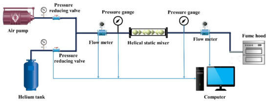
Figure 4.
Schematic diagram of gas mixing of helical static mixer model.
Model Validation
In the experiment, the number of mixing units of the helical static mixer is seven. Since the flow of the mixed gas is a steady incompressible flow, which satisfies the Bernoulli principle, so its expression of equation is as follows [36]:
where
P—Pressure loss (Pa)
ρ—Density (kg/m3)
v—Fluid velocity (m/s)
g—Acceleration of gravity (m/s2)
h—Height (m)
const—Constant.
Further, we define the inlet pressure of the helical static mixer is P1, the outlet pressure is P2 and the inlet velocity is v1, the outlet velocity is v2. In addition, we assume that the fluid outlet velocity v2 is λ times that of inlet velocity v1, its expression is as follows:
where
v2 = λv1
qv1—Inlet flow rate (m3/s)
qv2—Outlet flow rate (m3/s)
D—Equivalent diameter (m)
A—Cross-sectional area (m2)
Therefore, from Equation (8) we can further obtain the following expression:
Figure 5 presents the relationship between the inlet flow rate and pressure loss between the inlet and outlet of the helical static mixer. The tube pressure loss between the inlet and outlet of helical static mixer is increasing as the inlet flow rate increases. Through experiments and numerical simulation analysis, the accuracy of the three-dimensional model is verified.
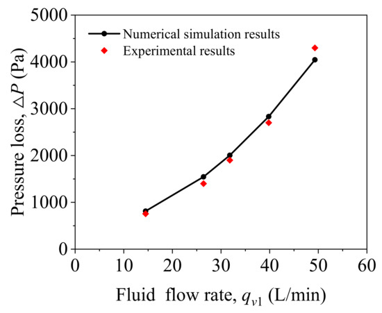
Figure 5.
Verification of experimental results and numerical simulation results.
4. Results and Discussion
Through the experimental research mentioned above, the reliability of the numerical simulation and experimental results has been verified for the helical static mixer model, and further parametric discussion of this model is carried out. As the number of mixing units, the torsion angle of the mixing units and the distance of the mixing units are important to determine the helical static mixer performance, parametric study has been conducted to investigate the effects of pressure loss and coefficient of variation changes of natural gas mixed with hydrogen. In addition, we also further discuss the radial velocity and the change of methane volume fraction of the outlet section of the helical static mixer. Considering the symmetry condition, we choose the data in the radius direction to study.
4.1. Effect of the Number of Mixing Units
In order to investigate the effect of number of mixing units N on the mixing characteristics of methane and hydrogen in the helical static mixer under the steady flow, which includes pressure loss between inlet and outlet in the helical static mixer, the proportion of methane composition and the change of outlet coefficient of variation, N is varied from 0 to 7 while other conditions are fixed in Table 6. The study of this section under the condition of hydrogen mixing ratio at 20% (The volume fraction of methane in the mixed phased is 80%) that achieved by the methane inlet velocity 3 m/s and hydrogen inlet velocity 0.75 m/s.
Table 6.
Related parameters of different mixing units of helical static mixer.
Figure 6 shows the variation of pressure loss and COV with the number of mixing units. As the number of units increases, the pressure loss of the helical static mixer gradually increases, while the coefficient of variation (COV) continues to decrease. When the number of mixing units is two, the COV value is 2.13%. When the number of mixing units is three, the COV value is 1.45%. Considering the application cost, three units is more appropriate. The coefficient of variation with three mixing units is 1.45%, and the pressure loss is 52.8 Pa. Figure 7 shows the methane volume fraction (Phase 1) of outlet section with different number of mixing units. With the number of mixing units increasing, the methane component concentration distribution becomes more uniform. Without the mixer, the outlet methane is obviously stratified, i.e., 80% of methane is mainly concentrated in the middle and lower parts while the upper part is mainly hydrogen. Correspondingly, the coefficient of variation (COV) reaches its maximum of 10.3%. On the other hand, the volume fractions of methane for five and seven units are stable at about 80%.
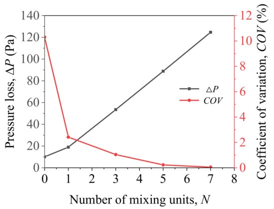
Figure 6.
Pressure loss and coefficient of variation (COV) change with different number of mixing units.
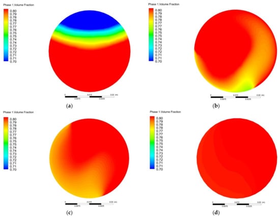
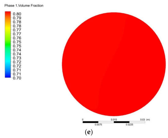
Figure 7.
Variation of outlet section methane volume fraction with different mixing units: (a) N = 0; (b) N = 1; (c) N = 3; (d) N = 5; (e) N = 7.
4.2. Effect of the Torsion Angle of Mixing Unit
As mentioned above, the units inside the mixer are arranged perpendicular to each other at 90°, and the numerical simulation results prove that the three units structure performs better in the mixing of the natural gas with hydrogen. Therefore, the mixing characteristics of methane and hydrogen under different torsion angles θ (θ = 60°,90°, 120°, 150°, 180°) in a three units helical static mixer are further studied. Figure 8 depicts the torsion angle arrangements, and the effect of the torsion angle θ on the pressure loss and the coefficient of variation during the mixing process through numerical simulation is further investigated. Table 7 presents the boundary condition parameters set in the numerical simulation process. The numerical simulation process is still carried out under the condition of 20% hydrogen mixing ratio.
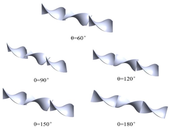
Figure 8.
Schematic diagram of the arrangement model of different torsion angles (60°, 90°, 120°, 150°, and 180°).
Table 7.
Numerical simulation boundary conditions related parameters of 3-units helical static mixer.
It can be seen from Figure 9 that as the torsion angle θ of the mixing unit arrangement increases, the pressure loss of the helical static mixer decreases with the torsion angle. When θ = 180°, it has a minimum value of 38.1 Pa. The coefficient of variation shows a trend of first decreasing and then increasing as the torsion angle increases. When the torsion angle θ = 120°, the COV minimum value is 0.66%. When θ = 60°, the maximum value of COV is 8.54%.
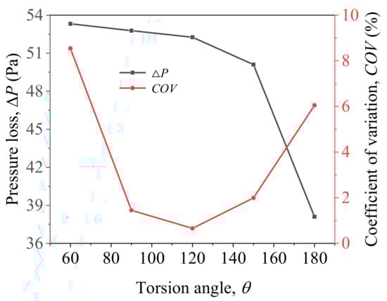
Figure 9.
Pressure loss and COV change with different torsion angle.
Figure 10 shows the influence of different torsion angles on the outlet methane volume fraction. As shown in Figure 10, the methane volume fraction with a torsion angle of 60° has the largest amplitude range. The changes in the methane volume fraction with torsion angles of 90° and 120° are stable, i.e., the methane volume fraction fluctuates quite little around 80%. When the torsion angle is 180°, the outlet methane volume fraction exhibits obvious stratification with the coefficient of variation (COV) of 6%. Considering the coefficient of variation and pressure loss parameters, it is more appropriate to select the torsion angle of 120°.
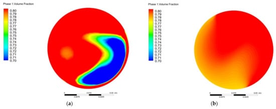
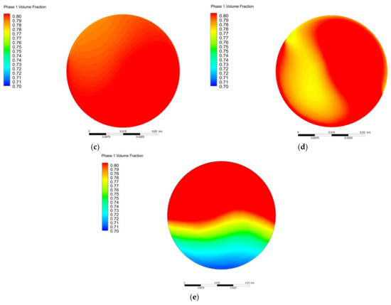
Figure 10.
Variation of outlet methane volume fraction with different torsion angle: (a) θ = 60°; (b) θ = 90°; (c) θ = 120°; (d) θ = 150°; (e) θ = 180°.
4.3. Effect of Mixing Units Distance
In order to explore the gas mixing characteristics, different distance conditions of mixing units are set. According to the different distances of the mixing units, we have established four 3D models with different distances. The distances between different mixing units are marked as (i = 1, 2). Figure 11 shows the schematic diagram of different mixing unit distances. From the figure, it can be seen that the Case A, Case B, Case C, and Case D are selected for investigating the influence of the distances of the mixing units on the gas mixing effect of the helical static mixer. Figure 12 shows the pressure loss and coefficient of variation of the four solutions with the distances of the mixing units. The pressure loss of the four programs has little change. However, Case A has the smallest COV value, and Case C has the largest COV value.
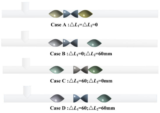
Figure 11.
Schematic diagram of different mixing units distance: (Case A: ; Case B: ; Case C: ; Case D: ).
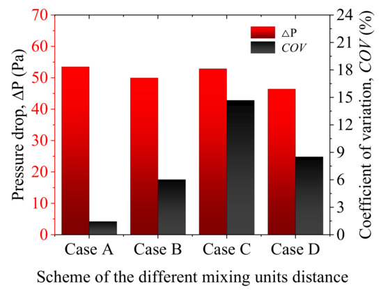
Figure 12.
Pressure loss and COV change with different arrangements.
Figure 13 shows the change of the outlet methane volume fraction for different arrangements. Among the four arrangements, the outlet methane volume fractions of Case B and Case C change more strongly. Essentially, the hydrogen in Case B, Case C, and Case D is mainly concentrated in the middle. Hence, the arrangement of mixing units has a great influence on the mixing behavior and Case A is relatively better with less fluctuation.
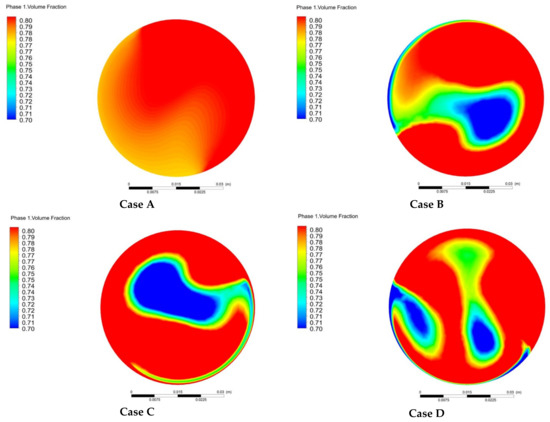
Figure 13.
Variation of outlet methane volume θ fraction with different arrangements: (Case A: ; Case B: ; Case C: ; Case D: ).
5. Conclusions
In this paper, the feasibility of hydrogen blended to natural gas via the helical static mixer in gas network is verified. The mixing of natural gas and hydrogen through the gas network can be widely used in gas stations, factories, domestic, and commercial appliances. The addition of the gas mixer proposed in this article will improve the stratification of the gas mixture, meanwhile the pressure loss of the pipe will not increase too much. According to the multiphase flow mixing evaluation index and numerical calculation method, this article discusses the influence of the number of mixing units, the torsion angle, and the distance of mixing units on the gas–gas (Methane–Hydrogen) mixing. Further, the optimization design criteria for the structure of the mixing device for the natural gas mixed with hydrogen system are proposed to provide a guiding baseline for the subsequent industrial operation. Through the above analysis, following conclusions are obtained:
- (1)
- The pressure loss increases with the number of mixing units increases, while the coefficient of variation gradually decreases. There is an optimum number of mixing units for a good mixing performance with relatively lower pressure loss. Based on our results, optimum number of mixing units are three, corresponding to the pressure loss of 52.8 Pa and the coefficient of variation of 1.45%.
- (2)
- As the torsion angle θ (θ = 60°, 90°, 120°, 150°, and 180°) increases, the coefficient of variation firstly decreases and then increases, while the pressure loss keeps decreasing. When θ = 120°, the COV has a minimum value of 0.66% and the pressure loss become 52.26 Pa.
- (3)
- Through the comparison of the three arrangements, it is found that the distance of the mixing unit has little effect on the pressure loss of the helical static mixer but has a greater effect on the coefficient of variation. The coefficient of variation (COV) from Case A to Case D increases first and then decreases, with a maximum value of 14.68% at Case C and a minimum value of 1.45% at Case A. Therefore, Case A (consecutive arrangement) is most appropriate.
Author Contributions
Conceptualization, C.C. and M.K.; funding acquisition, C.C.; methodology, S.F. and Q.X.; software, S.F.; validation, M.K. and S.F.; formal analysis, M.K. and Z.P.; resources, Z.G.; writing—original draft preparation, M.K.; All authors have read and agreed to the published version of the manuscript.
Funding
This research was funded by Natural Science Foundation of Zhejiang Province (No. LY20E060007).
Data Availability Statement
Data sharing is not applicable to this article.
Conflicts of Interest
The authors declare no conflict of interest.
References
- Forest, C.G.B.W. Effect of hydrogen addition on the performance of methane-fueled vehicles. Part I: Effect on S.I. engine performance. Int. J. Hydrogen Energy 2001, 26, 55–70. [Google Scholar]
- Karim, G.A.; Wierzba, I.; Al-Alousi, Y. Methane-hydrogen mixtures as fuels. Int. J. Hydrogen Energy 1996, 21, 625–631. [Google Scholar] [CrossRef]
- Sierens, R.; Rosseel, E. Variable Composition Hydrogen/Natural Gas Mixtures for Increased Engine Efficiency and Decreased Emissions. J. Eng. Gas Turbines Power 2000, 122, 135–140. [Google Scholar] [CrossRef]
- Chugh, S.; Posina, V.A.; Sonkar, K.; Srivatsava, U.; Sharma, A.; Acharya, G.K. Modeling & simulation study to assess the effect of CO2 on performance and emissions characteristics of 18% HCNG blend on a light duty SI engine. Int. J. Hydrogen Energy 2016, 41, 6155–6161. [Google Scholar] [CrossRef]
- Deng, J.; Ma, F.; Li, S.; He, Y.; Wang, M.; Jiang, L.; Zhao, S. Experimental study on combustion and emission characteristics of a hydrogen-enriched compressed natural gas engine under idling condition. Int. J. Hydrogen Energy 2011, 36, 13150–13157. [Google Scholar] [CrossRef]
- Singh, A.P.; Pal, A.; Agarwal, A.K. Comparative particulate characteristics of hydrogen, CNG, HCNG, gasoline and diesel fueled engines. Fuel 2016, 185, 491–499. [Google Scholar] [CrossRef]
- Genovese, A.; Contrisciani, N.; Ortenzi, F.; Cazzola, V. On road experimental tests of hydrogen/natural gas blends on transit buses. Int. J. Hydrogen Energy 2011, 36, 1775–1783. [Google Scholar] [CrossRef]
- Luo, S.; Ma, F.; Mehra, R.K.; Huang, Z. Deep insights of HCNG engine research in China. Fuel 2020, 263, 116612–116629. [Google Scholar] [CrossRef]
- Melaina, M.W.; Sozinova, O.; Penev, M. Blending Hydrogen into Natural Gas Pipeline Networks: A Review of Key Issues. Durability 2013, 1, 17–34. [Google Scholar] [CrossRef]
- Xiang, L.; Jiang, H.; Ren, F.; Chu, H.; Wang, P. Numerical study of the physical and chemical effects of hydrogen addition on laminar premixed combustion characteristics of methane and ethane. Int. J. Hydrogen Energy 2020, 45, 20501–20514. [Google Scholar] [CrossRef]
- Wang, J.; Huang, Z.; Tang, C.; Miao, H.; Wang, X. Numerical study of the effect of hydrogen addition on methane–air mixtures combustion. Int. J. Hydrogen Energy 2009, 34, 1084–1096. [Google Scholar] [CrossRef]
- Gimeno-Escobedo, E.; Cubero, A.; Ochoa, J.S.; Fueyo, N. A reduced mechanism for the prediction of methane-hydrogen flames in cooktop burners. Int. J. Hydrogen Energy 2019, 44, 27123–27140. [Google Scholar] [CrossRef]
- De Vries, H.; Levinsky, H.B. Flashback, burning velocities and hydrogen admixture: Domestic appliance approval, gas regulation and appliance development. Appl. Energy 2020, 259, 114116. [Google Scholar] [CrossRef]
- Wojtowicz, R. An analysis of the effects of hydrogen addition to natural gas on the work of gas appliances. Nafta Gaz 2019, 75, 465–473. [Google Scholar] [CrossRef]
- Zhao, Y.; McDonell, V.; Samuelsen, S. Experimental assessment of the combustion performance of an oven burner operated on pipeline natural gas mixed with hydrogen. Int. J. Hydrogen Energy 2019, 44, 26049–26062. [Google Scholar] [CrossRef]
- Zhao, Y.; McDonell, V.; Samuelsen, S. Influence of hydrogen addition to pipeline natural gas on the combustion performance of a cooktop burner. Int. J. Hydrogen Energy 2019, 44, 12239–12253. [Google Scholar] [CrossRef]
- Witkowski, A.; Rusin, A.; Majkut, M.; Stolecka, K. Analysis of compression and transport of the methane/hydrogen mixture in existing natural gas pipelines. Int. J. Press. Vessel. Pip. 2018, 166, 24–34. [Google Scholar] [CrossRef]
- Ogden, J.; Jaffe, A.M.; Scheitrum, D.; McDonald, Z.; Miller, M. Natural gas as a bridge to hydrogen transportation fuel: Insights from the literature. Energy Policy 2018, 115, 317–329. [Google Scholar] [CrossRef]
- Quarton, C.J.; Samsatli, S. Should we inject hydrogen into gas grids? Practicalities and whole-system value chain optimisation. Appl. Energy 2020, 275, 115172. [Google Scholar] [CrossRef]
- Wahl, J.; Kallo, J. Quantitative valuation of hydrogen blending in European gas grids and its impact on the combustion process of large-bore gas engines. Int. J. Hydrogen Energy 2020, 45, 32534–32546. [Google Scholar] [CrossRef]
- Nordio, M.; Wassie, S.A.; Van Sint Annaland, M.; Pacheco Tanaka, D.A.; Viviente Sole, J.L.; Gallucci, F. Techno-economic evaluation on a hybrid technology for low hydrogen concentration separation and purification from natural gas grid. Int. J. Hydrogen Energy 2020. [Google Scholar] [CrossRef]
- Judd, R.; Pinchbeck, D. Hydrogen Admixture to The Natural Gas Grid. In Compendium of Hydrogen Energy; Ball, M., Basile, A., Veziroğlu, T.N., Eds.; Woodhead Publishing: Oxford, UK, 2016; pp. 165–192. [Google Scholar] [CrossRef]
- Haeseldonckx, D.; D’haeseleer, W. The use of the natural-gas pipeline infrastructure for hydrogen transport in a changing market structure. Int. J. Hydrogen Energy 2007, 32, 1381–1386. [Google Scholar] [CrossRef]
- Zidouni, F.; Krepper, E.; Rzehak, R.; Rabha, S.; Schubert, M.; Hampel, U. Simulation of gas–liquid flow in a helical static mixer. Chem. Eng. Sci. 2015, 137, 476–486. [Google Scholar] [CrossRef]
- Rabha, S.; Schubert, M.; Grugel, F.; Banowski, M.; Hampel, U. Visualization and quantitative analysis of dispersive mixing by a helical static mixer in upward co-current gas–liquid flow. Chem. Eng. J. 2015, 262, 527–540. [Google Scholar] [CrossRef]
- Das, M.D.; Hrymak, A.N.; Baird, M.H.I. Laminar liquid–liquid dispersion in the SMX static mixer. Chem. Eng. Sci. 2013, 101, 329–344. [Google Scholar] [CrossRef]
- Hammoudi, M.; Si-Ahmed, E.K.; Legrand, J. Dispersed two-phase flow analysis by pulsed ultrasonic velocimetry in SMX static mixer. Chem. Eng. J. 2012, 191, 463–474. [Google Scholar] [CrossRef]
- Lobry, E.; Theron, F.; Gourdon, C.; Le Sauze, N.; Xuereb, C.; Lasuye, T. Turbulent liquid–liquid dispersion in SMV static mixer at high dispersed phase concentration. Chem. Eng. Sci. 2011, 66, 5762–5774. [Google Scholar] [CrossRef]
- Couvert, A.; Sanchez, C.; Charron, I.; Laplanche, A.; Renner, C. Static mixers with a gas continuous phase. Chem. Eng. Sci. 2006, 61, 3429–3434. [Google Scholar] [CrossRef]
- Zhuang, Z.; Yan, J.; Sun, C.; Wang, H.; Wang, Y.; Wu, Z. The numerical simulation of a new double swirl static mixer for gas reactants mixing. Chin. J. Chem. Eng. 2020, 28, 2438–2446. [Google Scholar] [CrossRef]
- Montante, G.; Coroneo, M.; Paglianti, A. Blending of miscible liquids with different densities and viscosities in static mixers. Chem. Eng. Sci. 2016, 141, 250–260. [Google Scholar] [CrossRef]
- Yang, X.; Zhao, L.; He, Z.; Dong, S.; Tan, H. Comparative study of combustion and thermal performance in a swirling micro combustor under premixed and non-premixed modes. Appl. Therm. Eng. 2019, 160, 114110. [Google Scholar] [CrossRef]
- Ozturk, M.; Dincer, I. Development of renewable energy system integrated with hydrogen and natural gas subsystems for cleaner combustion. J. Nat. Gas Sci. Eng. 2020, 83, 103583. [Google Scholar] [CrossRef]
- Thakur, R.K.; Vial, C.; Nigam, K.D.P.; Nauman, E.B.; Djelveh, G. Static Mixers in the Process Industries—A Review. Chem. Eng. Res. Des. 2003, 81, 787–826. [Google Scholar] [CrossRef]
- Mansour, M.; Liu, Z.; Janiga, G.; Nigam, K.D.P.; Sundmacher, K.; Thévenin, D.; Zähringer, K. Numerical study of liquid-liquid mixing in helical pipes. Chem. Eng. Sci. 2017, 172, 250–261. [Google Scholar] [CrossRef]
- Wallis, G.B. The averaged bernoulli equation and macroscopic equations of motion for the potential flow of a two-phase dispersion. Int. J. Multiph. Flow 1991, 17, 683–695. [Google Scholar] [CrossRef]
Publisher’s Note: MDPI stays neutral with regard to jurisdictional claims in published maps and institutional affiliations. |
© 2021 by the authors. Licensee MDPI, Basel, Switzerland. This article is an open access article distributed under the terms and conditions of the Creative Commons Attribution (CC BY) license (https://creativecommons.org/licenses/by/4.0/).