Abstract
Coal heavy-haul railway has been aiming at maximizing capacity utilization, but ignoring energy consumption for a long time. With the focus on green production, heavy-haul railways need transportation organization plans that can balance energy consumption and capacity utilization. Based on this, this paper proposes a data mining + optimization framework that uses train trajectory data to estimate train energy consumption and then uses a mixed integer programming model to simultaneously optimize plans from energy and capacity aspects. We use Gaussian distribution to describe features of energy consumption under different situations, and build a multi-dimensional cube to store these features to connect with the optimization model. In addition, a branch-and-bound algorithm is design to solve the optimization model. From the sensitivity analyses we can conclude that (1) shortening the departure interval from 13 min to 9 min will generate more energy consumption, about 3.6%; (2) combining short-form trains (50 units) with long-form trains (100 units) while increasing the carrying capacity will generate more energy consumption, about 5~14%; and (3) by controlling weights of the optimization model, capacity–energy-balanced plans can be obtained. The results can contribute to improving the sustainability of railways.
1. Introduction
1.1. Research Background
In the coal transportation system, heavy-haul railways have been the backbone because of their high capacity for a long time. In general, maximizing the utilization of the capacity of heavy-haul railway is the main objective of operations. The most common way to achieve this objective is by a pattern that combines two short-form trains (50 units) into one long form train (100 units). However, in daily operation, it is found that although the combination can effectively increase traffic density (which leads to a high ratio of capacity utilization), it also generates more energy consumption. With the focus on green production, it is inadvisable for meeting the capacity utilization or the optimal use of energy consumption unilaterally. Heavy-haul railways are in urgent need of transportation organization solutions that can balance energy consumption and capacity utilization.
However, there are challenges in describing distributions of energy consumption of heavy-haul systems in different dimensions and in depicting the relationship between energy consumption and capacity utilization, and thus in participating in the capacity utilization planning process:
- Although a series of automatic management and control platforms has been deployed in the railway system, the existing research still lacks ways of using these data. It is difficult to depict and analyze the distribution of train energy consumption under conditions of varying directions, time periods, and origin and destination, etc.
- The relationship between energy consumption and capacity utilization is difficult to determine, and there is a lack of transportation organization programming techniques that take both into account.
Motivated by these two problems, this paper proposes a data mining + optimization framework that uses train trajectory data (TTD) to estimate train energy consumption and then uses a mixed integer programming model to simultaneously optimize plans from energy and capacity aspects. We use Gaussian distribution to describe features of energy consumption under varying situations, and build a multi-dimensional cube to store these features to connect with the optimization model. In addition, a branch-and-bound algorithm is designed to solve the optimization model.
1.2. Research Overview
Developing models for assessing the energy consumption of rail freight has received significant attention since the 1970s [1,2,3]. Nowadays, many energy-oriented models are devoted to assessing the energy consumption/air pollution of rail transportation [4,5]. The energy models for freight transportation can be categorized into three types. The first type of model is analytical models, which can be used to estimate emissions of trains based on some assumed stochastic processes [6,7]. The second type of model is based on optimization models [8,9]). These models typically can model the microscopic movement of trains, which is critical for estimating accurate fuel consumption and emissions [10]. Energy-efficient rail train control and management decisions can also be incorporated into the models to analyze the environmental impact of railway movement [11,12,13]. The method to estimate the emissions differs by agency or rail class. The third group of models includes simulation-based approaches [14,15,16]. For example, the train energy model (TEM) that is widely used in the railway community is an effective tool to estimate the energy consumption of trains [17].
When the demand for transportation was greater than the supply, how to maximize the theoretical capacity of the line was the focus of research, and relatively little research was done on energy consumption. Under the new situation of energy conservation and low-carbon environmental protection, countries around the world are paying increasing attention to the construction and development of railways, further highlighting the energy-saving advantages of railways. Although railway transportation provides strong protection for economic development, its energy consumption problem has also become the focus of attention and research among all countries. The existing studies have shown that factors such as the hours a train runs in a network and the headway time affect the energy consumption of the train [18]. In the past, scholars’ research on railway energy consumption was mainly focused on energy consumption calculation, train operation, and control models and algorithms, and there are few studies that correlate the operation diagram with railway energy consumption. Representative works of the abovementioned studies on railway capacity, preparation of transport organization, and energy consumption of trains are shown in Table 1.

Table 1.
Representative literature on the study of railway capacity, preparation of transportation organization, and energy consumption of trains.
The above studies have played roles in the organization of heavy-haul railway transportation, but there are still some gaps, mainly in the capacity–energy relationship: (1) These studies are generally based on microscopic plans before operation, with little research on energy consumption under actual operating conditions. The models they are based on consider the ideal horizontal and vertical slope, with the calculated energy consumption being the reference value prior to operation. The actual energy consumption of the heavy-haul system is poorly depicted and the estimated value differs greatly from the reality. (2) There is a lack of multidimensional energy consumption models that can be used for transportation organization optimization. There is an inability to accurately portray the impact of different dimensions such as OD (volume from Origin to Destination), running time, and load on energy consumption. (3) There is a lack of models for the simultaneous optimization of capacity and energy consumption.
1.3. Main Article Contributions
In order to fill the gaps, in this paper we propose a framework with data analysis methods for estimating the distribution of energy consumption in different dimensions and a mixed integer programming model is used to obtain solutions that can balance capacity and energy consumption. The contributions can be summarized as follows:
- According to methods based on kinematic theory, an energy consumption calculation approach based on TTD is proposed, then the multidimensional energy consumption values are obtained, which include dimensions such as train forms and routes, etc. In order to solve the problem that the discrete energy consumption value cannot support the requirement of continuity of the objective function in the optimization model, we adopt Gaussian distributions under different dimensions as regression models to fit discrete energy consumption points and construct a distribution model with dimensions for the capacity- and energy-balanced optimization model.
- A simultaneous optimization model for timetable scheduling is proposed, considering objectives including capacity and energy consumption and constraints such as section carrying capacity, station loading and unloading capacity, and station recombination capacity, as well as the different energy consumption characteristics of different train paths. The model is based on a time–space network and the granularity on time can be brought down to 5 min. According to the energy consumption multi-dimensional distribution model, edge weights of the network are set. By means of finding and resolving conflicts in the timetable, we propose a branch-and-bound algorithm to solve the model.
- By comparing and analyzing experiments, some quantitative and qualitative patterns were discovered. This can guide future plan scheduling.
The remainder of this paper is organized as follows: In Section 2, we introduce the principles and methods of energy consumption calculation, and a multi-dimensional consumption cube is built in this section. Based on the cube, in Section 3, a mixed integer programming model to simultaneously optimize plans from energy and capacity aspects is illustrated. In Section 4, we make some cases to compare energy consumptions and energy utilizations in varying conditions and discuss the reasons. Section 5 gives conclusions about the research.
2. Framework and Methods for Energy Consumption Estimation
Traction phases are the basic conditions during train operation and include acceleration (TA), coasting (CO), and braking (TB). Different traction phases have different energy consumptions. For this reason, the methods studied in this section start with the detection of traction phases and then we design the energy consumption calculation methods on the basis of the traction phases. To ensure the validity of the calculation results, some data management and noise cleaning methods are designed in the procedure of calculating energy consumption. The designed calculation procedure includes:
- (1)
- TTD series data formation. This includes data pre-processing and formatting to time series data.
- (2)
- State-based traction phase detection. This is combined with the transformation method of traction phase identification; the discrete data points in TTD data are transformed into continuous sequence segments.
- (3)
- Noise cleaning of the TTD data for each traction phase. Correction of the data in each traction phase is completed using the Kalman filter.
- (4)
- Energy consumption measurement method based on traction phases. Individual methods for calculating the energy consumption of trains under traction phases are designed.
- (5)
- Multi-dimensional distribution model of energy consumption based on Gaussian distribution. This is based on the assumption of Gaussian distribution. The energy consumption distribution pattern is analyzed and the energy consumption model is established.
The flow of the energy consumption estimation is shown in Figure 1.

Figure 1.
Logical framework for calculating energy consumption standards based on data mining.
2.1. Data Preparation
This section provides a data structure for the corresponding data in order to standardize the description of the formulae in the model and algorithm later on. The notations involved are shown in Table 2.
Table 2.
Definitions.
This part uses data that include TTD data and line longitudinal and cross-sectional data. The TTD data contain detailed records of the number of trains, locomotive type, routing, grouping information, load information, kilometer sign, distance to the station ahead, ground signals, train operation speed, operation status, and other data during the operation of the train. The line longitudinal and cross-sectional data record parameters such as elevation differences, spatial position, and curve radius. The integration of the two can support the measurement of energy consumption.
The original TTD data contain various pieces of information during the train operation. We need to extract effective data reflecting the train speed, distance, time, and operation conditions. Data pre-processing is also carried out on the longitudinal and cross-sectional data to form a time series with the TTD series data in order to complete the data structure design.
TTD data are time series data, which can be expressed as
where is the TTD data set, is the corresponding data point. is the number of data points, is the time and minute at time , is the train position at time , is the train speed at time , and is the train status at time .
The longitudinal and cross-sectional data are in the form of spatial sequences. The elevation and the curve radius can be expressed respectively as follows:
where and are spatial positions, is the number of segments of elevation difference, is the number of segments of curve radius, is the kilometer sign at the end position of the train operation section, is the original elevation data, and is the original curve radius data. In order to fuse with the TTD data of time series, the longitudinal and cross-sectional data were discretized into time series from moment 1 to moment t as follows:
where is the longitudinal and cross-sectional data and is the longitudinal and cross-sectional data point at .
Through the above steps, the sequence, which records the train operation status, and the sequence, which records the line change condition, can be obtained. In the subsequent steps, the will be detected for the traction phases and the energy consumption will be calculated according to the detected phases segment.
2.2. Traction Phase Detection
The processed TTD data contain a large amount of discrete and fragmented train state information, such as adding front traction, unloading traction, unloading front traction, unloading rear traction, etc. These states can be divided into acceleration, coasting, and braking to facilitate the calculation of energy consumption. In this part, the train state is detected one by one according to the time sequence, and the data of the same state is divided into the same phase segment. The discrete original data is aggregated to extract the traction phase sequence, which can be used for the subsequent energy consumption calculation algorithm to calculate the energy consumption.
2.2.1. Traction Phases Definition
From the whole process of train operation, the operating curve of the heavy train in the coal lanes mainly consists of three parts: acceleration (TA), coasting (CO), and braking (TB). By identifying the state of discrete TTD data during train operation, it can be aggregated into continuous segments of traction service.
With train , the discrete data points during its operation can be expressed as:
where is the TTD data set of train , is the corresponding ith TTD data point, is the number of data points during train operation, is the hour and minute at time i, is the train position at time i, is the train speed at time I, and is the train status at time i.
By detecting continuity, traction phases can be obtained, which can be defined as
where is the set of traction phases of the train . is the information about the position (), moment (), speed (), curve radius (), longitudinal and cross-sectional elevation (), and type of traction phase () corresponding to the phases. is the number of traction phases contained in the train.
According to the above definition, the train status is detected one by one according to the time sequence. Through the designed corresponding relationship, the traction phase set can be obtained. The specific method is described in the next part.
2.2.2. State-Based Traction Phase Detection Method
According to the definition of the previous part, the traction phase segments of train operation can be aggregated according to the continuity of train operation state. TTD data can be used to comprehensively judge the traction phases according to acceleration, air duct pressure, engine speed, and other factors. When acceleration is positive and the engine is revving, it can be judged as traction; when the engine is not revving and the duct pressure is high, it can be judged as coasting; when the engine is not revving and the duct pressure is low, it can be judged as braking. (When the train needs to brake, the driver will turn the brake valve in the cab to the brake position to exhaust air, so as to reduce the air pressure of the train pipe. When the pressure of the auxiliary air cylinder of the train is greater than that of the train pipe, the slide valve is pushed to move so that the air in the auxiliary air cylinder enters the brake cylinder so as to push the brake shoe to generate braking force on the wheel and complete the braking operation.) Based on this, the mapping relationship for the traction phases can be designed as shown in Table 3.
Table 3.
Mapping relationship between train operation status and traction phases.
Under the premise of known TTD data and longitudinal and cross-sectional data, the running status of trains is detected one by one according to the chronological order of data points. If the train status has not changed, detection continues; if the train status has changed, the time and speed information of the current traction phase are recorded, and the detection of a new traction phase begins. The pseudo code of this process is shown in Algorithm 1.
| Algorithm 1. Phase detector algorithm. | |
| Input: TTD data DAL_s and level sequence data. | |
| Read TTD data table → DAL_s | |
| Read the sequence of planimetric sections→HoriVert_s | |
| Output: | |
| 1: | Marking train traction phases: Second_Phases→DAL_s [:].phases |
| 2: | Convert consecutive identical point phase codes to linear phase codes (discrete →continuous). |
| 2.1: | |
| 2.2: | Record the position of consecutive identical phase information by differencing the data before and after→pos pos=diff(DAL_s [:].phases) |
| 2.3: | Scan DAL_s, update while DAL_s[pos+1].phases == DAL_s[pos].phases do: = == = |
| 3: | Scanning of horizontal and vertical cross-sectional sequence data, update for i = 1: m do |
| = Func _Height();= Func _Height(); | |
| = Func _Cur (); | |
| Define the elevation function Func _Height, input the coordinates, and output the elevation of the current coordinate. define Func_Height(): | |
| Where HoriVert_s. | |
| return HoriVert_s. | |
| Define the curve function Func_Cur, input the coordinates, and output the curve radius of the current coordinate. define Func_Cur (): | |
| Where HoriVert_s. | |
| return HoriVert_s. | |
After processing by this algorithm, the original discrete data are aggregated into three main traction phases: acceleration (TA), coasting (CO), and braking (TB), which are then noise-cleaned and ready for energy consumption calculation.
2.3. TTD Data Noise Cleaning for Each Traction Phase
The position, speed, and other sensors in the TTD device have some noise in the actual production environment. The anomalous data caused by this noise have a large impact on the energy consumption calculation, so this paper used the Kalman filter to correct the data in each section of the traction phases based on the identification of traction phases to improve the credibility of the energy consumption calculation results.
Train operation is a dynamic process operated by the driver. Whenever the train status changes (such as cylinder pressure, tube pressure change, locomotive traction phase change, traction current change, etc.), the TTD device will automatically record a set of data. Based on the observation, there is a large number of jagged microscopic adjustment details in the data. On the basis of ensuring accuracy, in order to simplify the calculation process, this part assumes that the locomotive can be regarded as a uniformly accelerated motion when it is under the same traction phase. According to this hypothesis, it is straightforward to use Newtonian mechanics to infer the change in train position and speed at different moments.
Let be the current state, i.e., the vector consisting of position and velocity . When the state of the train at the previous moment t − 1 is known, the state of the train at the current moment t can be expressed according to the Newtonian mechanics formula as
where is the step size of the stage and is the acceleration of the train in that stage. The equation can also be expressed as
where is the state transfer matrix , and is the control matrix .
The acceleration of the train in this phase can be calculated by using the speed of the train at t − 2 and t − 1.
According to the Kalman filter principle, the covariance matrix can be used to represent the correlation between position and velocity, denoted by . This correlation is corrected at each moment by the correlation of the previous moment and the noise , which can be expressed as
The sensor data are assumed to obey a Gaussian distribution, the noise is represented by the covariance R, and the mean value of the Gaussian distribution is the read TTD data. The previously derived state projections are corrected based on the observations, and then
where is the weighted matrix for predicted residuals.
first weighs the magnitude of the predicted state covariance matrix Σ and the observed value matrix covariance R, and uses this to control whether the cleaning results favor the predicted model or the actual observed model. If the predictive model is favored, the data are cleaned more intensely and the cleaned data tend to be flat; conversely, the actual observed model is favored and the noise points can be tolerated and retained. The above process can be described by pseudo-code, expressed as shown in Algorithm 2.
| Algorithm 2. Kalman filter algorithm. |
| Input: TTD raw data |
| Read the TTD raw data table→ |
| Output: TTD date DAL_s |
| Save TTD date (DAL_s)→TTD data table |
| If the train traction phases (Phases) is the same as the previous tense |
| 1: Calculate |
| 2: Calculate optimal predictions |
| 3: Calculate the state transfer matrix |
| 4: Calculate the Kalman gain factor |
| 5: Correct best estimate |
| 6: Correct state transfer matrix |
| otherwise |
| 1: |
| 2: Calculat |
| Return , |
According to the above method, the noise of the TTD series data contained within each traction phase can be cleaned, and all the preparatory work before the energy consumption calculation is completed.
2.4. Method of Calculating Energy Consumption for Each Traction Phase
In this paper, according to the data obtained from the survey, the method introduced above was used to preprocess the data and detect the existing traction phases. This part calculates energy consumption by dynamic differential equations based on different traction phases (acceleration, coasting, braking). The energy consumption in each traction phase mainly includes (1) work done to overcome the train running resistance during train operation, (2) work done to overcome gravity, (3) increase in kinetic energy of the train, and (4) energy consumption of on-board equipment and other energy consumption. Since the energy consumption of on-board equipment and other energy consumption can be calculated according to the “Train Traction Calculation Regulations,” this part of the study treats them as known quantities.
The energy consumption calculation methods for different traction phases are as follows:
- Acceleration
During acceleration, the train locomotive converts the electrical energy in the grid into mechanical and internal energy. According to the principle of energy conservation and function, the energy consumption of train operation is equivalent to the sum of the mechanical energy change and the work done to overcome the total running resistance under the consideration of motor conversion efficiency . The functional transformation equation during the train operation can be described as follows:
where is the total mass of train , is the mass of train locomotive, is the final speed of train operation, is the initial speed of train operation, is the unit basic resistance of train vehicle, is the unit basic resistance of train locomotive, is the additional resistance of train curve, is the neutral acceleration, is the traction phase starting mileage position, is the traction phase ending mileage position, is the traction phase starting position elevation, is the traction phase ending position elevation, is the traction phase curve radius, and are the train running start and end time, is the supply voltage, and is the self-consumption of electricity.
The train running resistance includes basic running resistance and additional resistance. The first half of the formula is the basic resistance, which mainly includes the mechanical frictional resistance between the wheel axle and the wheel rail; the second half of the formula, , is the additional resistance, mainly air resistance, which has a square relationship with the running speed of the train, and is a quadratic polynomial with speed as an independent variable.
According to the railway traction calculation industry standard, empirical parameters can be used as the additional resistance of the curve.
- 2.
- Coasting
In the coasting phase, since the locomotive motor no longer applies tractive force, the tractive force does not do work and the train does work at the cost of mechanical energy (kinetic energy plus potential energy) consumption to overcome the train running resistance. Therefore, the energy consumption of the train only needs to consider the self-consumption of electricity by the locomotive instrumentation, and the specific expression is as follows:
where is the energy consumption value of train coasting phase, is the motor conversion efficiency, and are the train running start and stop times, respectively, is the supply voltage, and is the self-consumption of electricity.
- 3.
- Braking
As the braking method of the train studied in this paper is mainly gate braking and air braking, the motor does not output tractive force during the braking process, and the tractive force does not do any work. Therefore the train energy consumption only needs to consider the locomotive instrumentation self-use electricity consumption. The specific expression is as follows:
where is the energy consumption value of the train braking phase, is the motor conversion efficiency, and are the train running start and stop times, respectively, is the supply voltage, and is the self-consumption of electricity.
- 4.
- Total Energy Consumption
According to the above three train operation traction phases, the calculated can be regarded as the energy consumption generated by the train during operation, and A, B and C are the acceleration, braking, and coasting phases, respectively.
According to the above steps, the energy consumption data of each train can be mined and calculated based on the TTD data.
2.5. Multi-Dimensional Energy Consumption Distribution Model
Based on the above method, the energy consumption data of a single train can be obtained. Based on the assumption of Gaussian distribution, this part condenses the energy consumption standards contained therein to form a multi-dimensional distribution model for reference. The dimensions that determine the energy consumption include the train tonnage rating, different train groups, travel paths, the stopping scheme, etc. By calculating the traction energy consumption of trains according to different running modes, the influence of various conditions on the traction energy consumption of trains such as different destinations, different time periods, different sections, different fixed numbers, different stopping schemes, and different running speeds can be obtained. The above seven dimensions can be expressed as :
where represent the departure and arrival stations of the train, respectively, refer to the start and end time of the train operation, respectively, indicates the combination of train (including long-form train, short-form train, and empty train mode), takes the value to represent different stopping schemes of the train, and indicates the train operation speed, which refers to the train operation in the section, excluding the stopping time of intermediate stations and the additional time of starting and stopping. represents the energy consumption of a specific train under certain data conditions.
Let the individual energy consumption utilization of trains in the same dimension obey a Gaussian distribution, whose probability density function is noted as and can be expressed as:
Through data fitting techniques, the mean μ and variance of the energy consumption in different dimensions can be obtained to construct Gaussian distribution models. The resulting multi-dimensional distribution model dimensions are shown above.
3. Optimization Transportation Plans Considering Capacity and Energy Consumption
Considering constraints such as line interval passing capacity, station loading and unloading capacity, and combined dismantling capacity, this section calculates the energy consumption of trains on different routes based on the results of Section 2, and constructs an optimization model to obtain plans that can balance energy consumption and capacity utilization. An algorithm is designed to solve the model.
3.1. Model Building
3.1.1. Notation Definition
Before defining the parameters, the problem was first hypothesized and the scope of the study was defined.
Rail transportation is based on a 24 h decision cycle. Considering the scale of computing, it is necessary to divide the day into time periods expressed in several minutes, and in each time period the physical stations are replicated and expanded, and so on, forming a time–space network of nodes corresponding to the departure and arrival of heavy trains at each station at any given moment. The lines are assumed to be double lines, and the combined operation of long and short trains can only be performed in the combined stations. Under such assumptions, the relevant knowledge of graph theory was applied to the modeling analysis.
The key to solving the transportation organization optimization problem was to obtain the train operation plan and the specific transportation path for each demand. In view of this, the variables expressing the train operation plan and the transport path guidance variables for demand were designed, and the specific meanings are shown in Table 4. Among them, the upper corner markers in the transport path guidance variables for demand contained both the possible train arcs to take and the waiting arcs for loading or unloading, the stopping arcs after loading is completed, and the transfer arcs at the combination stations.
Table 4.
Model notation.
After determining the decision variables, a series of constraints was constructed, such as flow balance constraints, line and station capacity constraints, decision variables association constraints, combination station combination capacity constraints, combination train succession time constraints, etc., so as to form the transportation organization optimization model of the network flow optimization theory. The parameters involved in the model are detailed in Table 4.
3.1.2. Objective Function
The objective function considering the optimization of heavy-haul railway transportation organization in the coal lanes includes (1) travel distance cost, (2) energy consumption cost of heavy trains, and (3) running time cost, where objectives 1 and 3 represent capacity utilization and objective 2 represents energy consumption. Among them, the travel time and distance cost parameters can be obtained from the actual operation data, and the energy consumption cost parameters are obtained by using the analysis results in Section 2.
- (1)
- The cost of distance traveled by heavy trains is divided into two parts; one is the cost of the actual travel process, and the other is the economic cost of the combined operation.
- (2)
- The energy cost of heavy train transportation is divided into two parts; one is the energy cost spent during the actual travel and the other is the energy cost spent in the combined operation.
- (3)
- The running time span costs accounted for by the train operation plan. The parameter converts the time into other costs by putting energy consumption costs and the travel distance costs on the same scale.
The total objective function can be expressed as follows:
and
3.1.3. Constraints
- (1)
- Flow balance constraint. For an arbitrary demand , the transport path should be guaranteed to have a beginning and an end, as well as continuity in the path. The following three equations establish the flow balance constraints for the start node, intermediate nodes, and end node, respectively.
- (2)
- Establish a connection between the decision variables y and x. y is used to indicate whether an arc is used or not, and x is used to indicate whether a demand is conveyed by a certain arc.
- (3)
- Train loading capacity constraint. This cannot exceed the number of trains available for supply.
- (4)
- Combination station combination capacity constraint. During any time period, the combination station n completed operations cannot exceed the combination capacity of the station.
- (5)
- The section passing capacity constraint. For any section e, the number of trains released in a given time period cannot exceed the maximum passing capacity constraint of the section.
- (6)
- At a station, only one train can leave at most during a time period.
- (7)
- At a station, only one train can arrive at most during a time period.
- (8)
- Headway time constraint for a combination operation. The necessary time should be left between two adjacent trains for a combination operation, and the waiting time should not be too long.
- (9)
- Total demand constraint. The total amount of actual transportation should be exactly equal to the total amount of demand.
3.2. Branch-and-Bound Algorithm
Based on the Section 3.1, train time–space route analysis, the mixed integer programming model, including energy consumption and capacity, was established, and a branch-and-bound algorithm was designed to solve the model. The algorithm pseudo-code is shown in Algorithm 3.
| Algorithm 3. Branch-and-bound algorithm. | |
| Input: train information weighting factor objective function value factor, set of constraint parameters. | |
| Output: 0–1 decision variables 、, train running plans. | |
| 1: | Create a search space based on the seven dimensions of the variable . |
| 2: | Create a time–space network of railway operations and import information on |
| travel cost , energy cost , interchange cost , etc. | |
| 3: | Simplify the search space into a spatial tree. |
| 4: | Search for a feasible solution using a depth-first search strategy and define as |
| the current initial upper bound. | |
| 5: | Continuing the search for other feasible solutions using a breadth-first search |
| strategy, using the branch-and-bound algorithm. | |
| 5.1 Initialization: number of branches , , 5.2 if if go to 5.2 otherwise go to 5.6 otherwise Take the node with the smallest lower bound value from to become the current expanded node . 5.3 , expand all child nodes of the current expansion node Calculate the lower bound value of each child node , get node Delete the current expansion node 5.4 if All extended child nodes of current node are pruned, , go to 5.2 otherwise go to 5.5 5.5 if Add all nodes to node list Delete all nodes then go to 5.2 otherwise go to 5.6 5.6 if Select the optimal node in the node list to obtain the optimal solution otherwise go to 5.5 end | |
| 6: | After all nodes are searched, the algorithm ends, and the optimal train operation |
| plan is obtained | |
4. Numerical Experiments
In this paper, we calculated the actual energy consumption of trains operating on a line segment belonging to a group in northern China in November 2017. Among them, there were 23 stations on the main line excluding Station 25, of which there were four third-class stations, 19 fourth-class stations, and nine stations with 10,000 tons of feeder lines. The total length of the line was 264.6 km, with a maximum restricted slope of 10.9‰ and a maximum speed limit of 82 km/h.
In this paper, the data involved included (1) railway topology data, including railway lines and basic station data; (2) cross- and longitudinal section data, including line length, kilometer markers, gradient and curve radius, etc.; (3) TTD (train trajectory data) for that month. In Figure 2, Station 1–Station 25 is in the upstream direction whereas the opposite is downstream. Station 2, Station 3, Station 4, Station 9, Station 24, and Station 25 were the main loading stations, and trains mainly stopped at these stations. The types of trains included empty trains, short-form trains (50 units), and long-form train (100 units).
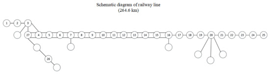
Figure 2.
Diagram of a line belonging to a group in northern China.
The numerical experiment mainly included (1) energy consumption calculations and the construction of a multi-dimensional distribution model, (2) a comparison of the average energy consumption of long- and short-form trains, (3) the effect of departure interval on the energy consumption of long trains, and (4) an analysis of the capacity and energy consumption.
4.1. Energy Consumption Calculations and Construction of Multi-Dimensional Distribution Model
The data in different dimensions (train origin and destination, time period, on-segment, fixed number, stopping scheme, operating speed, etc.) were extracted and used to calculate the energy consumption and analyze energy consumption criteria using the methods mentioned in this section. Due to the large number of dimensions involved, this section takes the interval of Station 24–Station 2 as an example, and the scatter plots of energy consumption for empty trains, short-form trains (50 units), and long-form trains (100 units) in this interval are shown in Figure 3a–c. The observation shows that even in the same dimension, there were differences in the energy consumption of trains, which may be due to (1) the variability of drivers’ driving behavior or (2) the variability due to the sparsity of train tracking in different time periods. The mean values of energy consumption excavation for different types of trains were 17,512.0 kw·h (short-form trains), 9479.9 kw·h (empty trains), and 51,351.6 kw·h (long-form trains), which generally shows that the energy consumption of the long-form train was the highest, the energy consumption of the empty trains was the lowest, and the difference in energy consumption between different empty trains was the smallest.
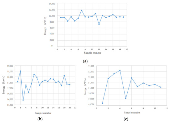
Figure 3.
Scatter diagram of energy consumption (kw∙h) of trains. The study section range is Station 24–Station 2 (a) for the short-form train, (b) for the empty train, and (c) for the long-form train.
The data under different dimensions were fitted separately for Gaussian distribution, and the fitting was done according to the 3σ criterion to determine the range, i.e., the set σ could contain 99.74% of the values in the interval [μ − 3σ, μ + 3σ]. The energy consumption of the individual trains existing in actual operation was calculated and classified and aggregated according to the dimensions, and a series of energy consumption data sets were obtained. The mean μ and standard deviation σ of energy consumption generated by train operation under some dimensions are shown in Table 5. The original station and destination station included Station 2, Station 3, Station 4, Station 9, Station 24, and Station 25. The number of stops was distributed in the range of 0–6, the train travel speed was concentrated in the range of 40–70 km/h, and the time period was in the range of 0–24 h. The closer the value of was to 1, the better the fitting effect was. The results show that was distributed between 0.69 and 0.87, and the overall fitting results were acceptable. The reason for the low fit of some dimensions is that the amount of data in some dimensions in the actual data was not enough, which led to a lack of fit.
Table 5.
Mean and standard deviation of energy consumption of train operation under partial conditions (energy unit: kw·h).
To show the form of the energy consumption criterion more concretely, Figure 4a–c shows the Gaussian distribution of empty, short-form trains (50 units) and long-form trains (100 units) using the Station 24–Station 2 interval as an example. By fitting the curves, it was possible to achieve continuation of discrete data to support subsequent decisions on transportation organization plans.
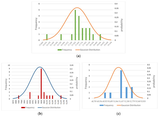
Figure 4.
The Gaussian distribution of energy consumption in the Station 24–Station 2 interval, where (a) is for short-form trains, (b) is for empty trains, and (c) is for long-form trains. The standard deviations are 935.3 kw·h (empty trains), 557.3 kw·h (short-form trains), and 856.2 kw·h (long-form trains).
Observing the parallel axis diagram of the multi-dimensional distribution model, when only a single dimension was considered, there was a certain pattern of energy consumption: The more stops in the same type of train, the greater the energy consumption, and similarly, the higher the speed in the same type of train, the greater the energy consumption, which is consistent with general common sense. However, when different combinations of dimensions were considered, the energy consumption distribution showed a staggered shape, and the relationship between its size and dimensionality was more complicated. Energy consumption distribution patterns of the upper and lower trains in seven dimensions are shown in Figure 5.
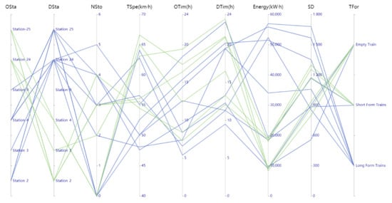
Figure 5.
Energy consumption distribution patterns of the upper and lower trains in seven dimensions.
Among them, OSta is the origin station, DSta is the destination station, NSta is the number of stops, and TSpe is the train travel speed. OTim is the departure time, DTim is the arrival time, TFor is the train combination form, Energy is the mean energy consumption, and SD is the standard deviation of energy consumption.
In order to clarify the relationship between dimension and energy consumption, we compared the average energy consumption of long and short trains, and analyzed the effect of departure interval on energy consumption of long-form trains.
4.2. Comparison of Average Energy Consumption of Long- and Short-Form Trains
In this section, the energy consumption of long-form trains and short-form trains with the same transportation capacity was measured in different characteristic intervals (long distance, short distance, large slope, small slope, etc.), and the results are shown in Figure 6 and Table 6.
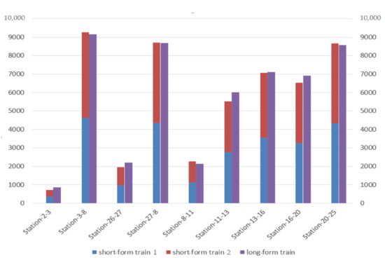
Figure 6.
Example of comparison between the capacity of a long-form train (100 units) and two short-form trains (50 units).
Table 6.
Comparison of energy consumption between a long-form train (100 units) and two short-form trains (50 units).
When in the short distance interval (e.g., Station 2–Station 3, Station 26–Station 27), the energy consumption of long-form trains was greater than that of short-form train with the same transportation volume; when in the large gradient interval (e.g., Station 16–Station 20, Station 11–Station 13), the energy consumption of long-form train was greater than that of short-form trains with the same transportation volume. For Station 26–Station 27, Station 16–Station 20 and Station 11–Station 13, the energy consumption of the long-form train was greater than that of the short-form train for the same transport volume; when in the long-distance interval (e.g., Station 3–Station 8, Station 20–Station 25), the energy consumption of the long-form train was greater than that of the short-form train. Similarly, the energy consumption of the long-form train was smaller than that of the short-form train in the case of small slope interval (e.g., Station 27–Station 8). Train energy consumption was smaller than that of the short-form train. The specific values can be seen in Table 6.
In summary, the combination of short-form trains into a long-form train in the interval with small spacing or large gradient generates more energy consumption (about 5~14%), although it can improve the traffic density and make full use of the passing capacity of the section; on the contrary, in the interval with large spacing or small gradient, the long-form train had certain advantages in energy consumption (about 1–5% can be saved).
4.3. The Effect of Departure Interval on Energy Consumption of Long Trains
In order to study the influence of the departure interval on energy consumption, the long-form train was selected as an example to calculate the average value of energy consumption under different departure intervals (as shown in Figure 7). When the departure interval was longer than 15 min, the trains on the line had less influence on each other, and the energy consumption of trains did not show great changes. If the interval was compressed, the average energy consumption increased as more trains were carried on the section line. For example, if the long-form train interval was compressed from 13 min to 9 min, the energy consumption increased by about 3.6%. Therefore, reducing the departure interval between trains may increase energy consumption while increasing the density and passing capacity.
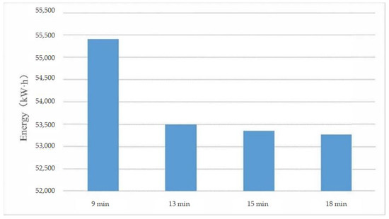
Figure 7.
Distribution of energy consumption for long-form trains with different departure intervals.
In summary, the setting of departure interval and the planning of long- and short-form train grouping affect the energy consumption values. By comparing the experiments, the relationship between capacity utilization decision variables and energy consumption can be found as follows:
- (1)
- Long-form trains generate more energy consumption when the departure interval is short or in a higher-gradient section. When the departure interval is short or in a higher-gradient section, combining short-form trains into a long-form train will generate more energy consumption (about 5–14% more), although it can improve the traffic density and passing capacity of the section; on the contrary, when the departure interval is long or in a lower-gradient section, a long-form train has a certain advantage in saving energy (about 1–5%).
- (2)
- Compressed departure intervals may cause an increase in energy consumption. For example, when compressing the departure interval of long-form trains, the energy consumption of a 9 min departure interval is higher by 3.6% compared to a 13 min departure interval.
4.4. Analysis of Capacity and Energy Consumption
The model solution results in Section 3 were influenced by the parameters , , and .
In this paper, we set up sensitivity analysis experiments to analyze the capacity and energy consumption in different scenarios by controlling parameters , , and in Equation (30). The experimental results are shown in Figure 8.
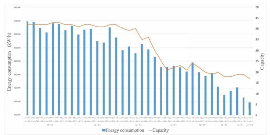
Figure 8.
Experiment on capacity energy utilization analysis.
By constantly changing the value of in the objective function, it was found that as the energy consumption influence parameter increased, the energy consumption of the plan decreased. The capacity value fluctuated and decreased when ≤ 0.3, from the maximum capacity of 43 trains, but the decreasing range was small, and the fluctuation range was between 40 and 43 trains. What is more, with the continuous increase of , the capacity decreased precipitously, which was much larger than that of the previous scenario. When ≥ 0.5, the capacity flattened out again.
It can be viewed that when , at which time the capacity value was 40 trains. However, as energy consumption continued to decrease, the capacity declined rapidly when the energy provided could not support a large number of trains running. Finally, with the reduction in energy consumption, although the capacity remained reduced, it did not change much.
To sum up, for heavy-haul railway systems, energy consumption and capacity can be optimized simultaneously under a parameter set (, , and ). The different parameters of capacity and energy consumption have influence on the plan, and the recommended train plan varies with the value. When the freight volume in the railway line does not reach the top capacity, the plans can be controlled to make the railway energy consumption level around . This way, the railway system can maintain a high level of capacity while minimizing the energy consumption.
5. Conclusions
In this paper, we studied railway coal transportation lanes. Based on the actual TTD data after the line operation and the longitudinal and cross-sectional information of the section where the trains are located, we used data analysis methods to find out the usage patterns of energy consumption, and use the mixed integer programming model to obtain a solution that can balance passing capacity and energy consumption. Specifically, it includes the following: (1) According to the kinematic model, train trajectory data (TTD) are used to depict energy consumption, including different tonnage ratings (tons, regular trains), different phases (acceleration, coasting, braking), and other cases. Through the assumption of Gaussian distribution, we analyzed its distribution pattern, obtained the relationship between energy consumption and the capacity, and obtained the specific energy consumption of multiple dimensions and high detail in different times and spaces, which could be used as the basis for the analysis of the objective function coefficients of the optimization model. (2) Based on time–space state network and the path analysis of train operation, a mixed integer programming model including energy consumption and capacity was established by comprehensively considering the constraints of section passing capacity, station loading and unloading capacity, and combined dismantling capacity. In addition, a branch-and-bound algorithm was designed to solve the model. (3) In this paper, we took a railway in northern China as an example to verify the method. (1) The mean value and standard deviation of train energy consumption with different stopping schemes, tonnage ratings, and combination types of empty and loaded vehicles on the line section were calculated. (2) According to the influencing factors of train energy consumption, the relationship between capacity utilization and energy consumption was analyzed. (3) Transport organization plans with a balanced consideration of capacity and energy consumption were obtained. Among them, according to sensitivity analyses, we concluded that (1) shortening the departure interval from 13 min to 9 min generates more energy consumption, about 3.6%; (2) combining short-form trains (50 units) into long-form trains (100 units) while increasing the traffic density and passing capacity also generates more energy consumption, about 5–14%; and (3) by controlling weights of the optimization model, capacity-energy-balanced plans can be obtained with .
In this paper, when constructing the railway organization optimization model, the influence of locomotive use, vehicle maintenance, and other factors on the train organization process was ignored, so further research can be conducted here. In the meantime, future research can further analyze railway field data comprehensively, so the energy consumption of trains operating in the station can be considered, and methods such as kinematic multi-mass models can be introduced to further improve the calculation of train energy consumption. Similarly, the traffic data used in the numerical experiments of this paper are of a specific period in a specific section, without considering the volatility of the traffic. The impacts of this capacity and energy consumption on train organization in extreme cases, i.e., periods of extreme capacity stress or extreme surplus, can be worth considering in future studies.
Author Contributions
Conceptualization, J.F.; methodology, J.F.; resources, J.F.; writing—original draft preparation, J.F.; writing—review and editing, J.F.; supervision, J.C.; validation, J.C. Both authors have read and agreed to the published version of the manuscript.
Funding
The research was supported by the National Natural Science Foundation of China (grant no. U1734204).
Institutional Review Board Statement
Not applicable.
Informed Consent Statement
Not applicable.
Data Availability Statement
Due to the nature of this research, the participants of this study did not agree for their data to be shared publicly.
Conflicts of Interest
The authors declare no conflict of interest.
References
- Assad, A. Analytical models in rail transportation: An annotated bibliography. INFOR Inf. Syst. Oper. Res. 1981, 19, 59–80. [Google Scholar] [CrossRef][Green Version]
- Assad, A. Analysis of rail classification policies. INFOR Inf. Syst. Oper. Res. 1983, 21, 293–314. [Google Scholar] [CrossRef]
- Bodin, L.D.; Golden, B.L.; Schuster, A.D.; Romig, W. A model for the blocking of trains. Transp. Res. Part B Methodol. 1980, 14, 115–120. [Google Scholar] [CrossRef]
- Kim, N.S.; Van Wee, B. Assessment of co2 emissions for truck-only and rail-based intermodal freight systems in europe. Transp. Plan. Technol. 2009, 32, 313–333. [Google Scholar] [CrossRef]
- Sieminski, A.; Energy Information Administration. International Energy Outlook 2016. Available online: https://www.csis.org/events/eias-international-energy-outlook-2016 (accessed on 12 January 2021).
- Knörr, W.; Seum, S.; Schmied, M.; Kutzner, F.; Anthes, R. Ecological Transport Information Tool for Worldwide Transports—Methodology and Data Update; IFEU: Heidelberg, Germany; INFRAS: Bern, Switzerland; IVE: Hannover, Germany, 2011. [Google Scholar]
- Jorgensen, M.W.; Sorenson, S.C. Estimating emissions from railway traffic. Int. J. Veh. Des. 1998, 20, 210–218. [Google Scholar] [CrossRef]
- Kirschstein, T.; Meisel, F. Ghg-emission models for assessing the eco-friendliness of road and rail freight transports. Transp. Res. Part B Methodol. 2015, 73, 13–33. [Google Scholar] [CrossRef]
- Zhou, X.; Tanvir, S.; Lei, H.; Taylor, J.; Liu, B.; Rouphail, N.M.; Frey, H.C. Integrating a simplified emission estimation model and mesoscopic dynamic traffic simulator to efficiently evaluate emission impacts of traffic management strategies. Transp. Res. Part D Transp. Environ. 2015, 37, 123–136. [Google Scholar] [CrossRef]
- Lindgreen, E.; Sorenson, S.C. Simulation of Energy Consumption and Emissions from Rail Traffic; Technical University of Denmark, Department of Mechanical Engineering: Kongens Lyngby, Denmark, 2005; ISBN 87-7475-328-1. [Google Scholar]
- Patterson, Z.; Ewing, G.O.; Haider, M. The potential for premium-intermodal services to reduce freight co2 emissions in the quebec city–windsor corridor. Transp. Res. Part D Transp. Environ. 2008, 13, 1–9. [Google Scholar] [CrossRef]
- Howlett, P.G.; Pudney, P.J. Energy-Efficient Train Control; Springer Science & Business Media: New York, NY, USA, 2012. [Google Scholar]
- Lukaszewicz, P. Energy saving driving methods for freight trains. Wit Trans. Built Environ. 2004, 74. [Google Scholar] [CrossRef]
- Cortés, C.E.; Vargas, L.S.; Corvalán, R.M. A simulation platform for computing energy consumption and emissions in transportation networks. Transp. Res. Part D Transp. Environ. 2008, 13, 413–427. [Google Scholar] [CrossRef]
- Heinold, A.; Meisel, F. Emission rates of intermodal rail/road and road-only transportation in europe: A comprehensive simulation study. Transp. Res. Part D Transp. Environ. 2018, 65, 421–437. [Google Scholar] [CrossRef]
- Wu, Q.; Spiryagin, M.; Cole, C. Train energy simulation with locomotive adhesion model. Railw. Eng. Sci. 2020, 1–10. [Google Scholar] [CrossRef]
- Drish, W.F., Jr. Train Energy Model—User’s Manual, Version 1.5; Railway Simulators; The National Academies of Sciences, Engineering, and Medicine: Washington, DC, USA, 1989. [Google Scholar]
- Ritzinger, U.; Puchinger, J.; Hartl, R.F. Dynamic programming based metaheuristics for the dial-a-ride problem. Ann. Oper. Res. 2016, 236, 341–358. [Google Scholar] [CrossRef]
- Cucala, A.P.; Fernandez, A.; Sicre, C.; Dominguez, M. Fuzzy optimal schedule of high speed train operation to minimize energy consumption with uncertain delays and driver’s behavioral response. Eng. Appl. Artif. Intell. 2012, 25, 1548–1557. [Google Scholar] [CrossRef]
- Domínguez, M.; Fernández-Cardador, A.; Cucala, A.P.; Gonsalves, T.; Fernández, A. Multi objective particle swarm optimization algorithm for the design of efficient ato speed profiles in metro lines. Eng. Appl. Artif. Intell. 2014, 29. [Google Scholar] [CrossRef]
- Xiang, L.; Hong, K.L. Energy minimization in dynamic train scheduling and control for metro rail operations. Transp. Res. Part B Methodol. 2014, 70, 269–284. [Google Scholar] [CrossRef]
- Chen, D.; Li, S.; Li, J.; Ni, S.; Liu, X. Optimal high-speed railway timetable by stop schedule adjustment for energy-saving. J. Adv. Transp. 2019, 2019, 1–9. [Google Scholar] [CrossRef]
- Zhang, H.; Jia, L.; Wang, L.; Xu, X. Energy consumption optimization of train operation for railway systems: Algorithm development and real-world case study. J. Clean. Prod. 2019, 214, 1024–1037. [Google Scholar] [CrossRef]
- Yang, X.; Chen, A.; Ning, B.; Tang, T. A stochastic model for the integrated optimization on metro timetable and speed profile with uncertain train mass. Transp. Res. Part B Methodol. 2016, 91, 424–445. [Google Scholar] [CrossRef]
- Bocharnikov, Y.V.; Tobias, A.M.; Roberts, C.; Hillmansen, S.; Goodman, C.J. Optimal driving strategy for traction energy saving on dc suburban railways. Iet Electr. Power Appl. 2007, 1, 675–682. [Google Scholar] [CrossRef]
- Yun, B.; Baohua, M.; Fangming, Z.; Yong, D.; Chengbing, D. Energy-efficient driving strategy for freight trains based on power consumption analysis. J. Transp. Syst. Eng. Inf. Technol. 2009, 9, 43–50. [Google Scholar] [CrossRef]
- Xiang, X.; Zhu, X. An optimization strategy for improving the economic performance of heavy-haul railway networks. J. Transp. Eng. 2016, 142, 04016001–04016003.04016013. [Google Scholar] [CrossRef]
- Medanic, J.; Dorfman, M.J. Energy efficient strategies for scheduling trains on a line. IFAC Proc. Vol. 2002, 35, 481–486. [Google Scholar] [CrossRef]
- Albrecht, T.; Oettich, S. A New Integrated Approach to Dynamic-Schedule Synchronization and Energy-Saving Train Control. In Computers in Railways VIII; WIT Press: Southampton, UK, 2002; Volume 61. [Google Scholar]
- Ghoseiri, K.; Szidarovszky, F.; Asgharpour, M.J. A multi-objective train scheduling model and solution. Transp. Res. Part B Methodol. 2004, 38, 927–952. [Google Scholar] [CrossRef]
- Sicre, C.; Cucala, P.; Fernández, A.; Jiménez, J.A.; Serrano, A.A. A Method to Optimise Train Energy Consumption Combining Manual Energy Efficient Driving and Scheduling. In Computers in Railways XII; WIT Press: Southampton, UK, 2010; Volume 114, pp. 549–560. [Google Scholar] [CrossRef]
- Lancien, D.; Fontaine, M. Computing train schedules to save energy: The mareco program. Rev. Gén. Chem. Fer 1981, 100, 679–692. [Google Scholar]


Publisher’s Note: MDPI stays neutral with regard to jurisdictional claims in published maps and institutional affiliations. |
© 2021 by the authors. Licensee MDPI, Basel, Switzerland. This article is an open access article distributed under the terms and conditions of the Creative Commons Attribution (CC BY) license (https://creativecommons.org/licenses/by/4.0/).