1. Introduction
The natural gas industry has undergone a rapid period of expansion in North America, mainly through unconventional resources production like shale gas. The key components that drove shale gas exploitation were technological improvements in drilling and production, and elevated natural gas prices (US Energy Information Administration) [
1]. Unconventional gas reservoirs are characterized by low permeability rocks, including tight sandstones, carbonates, coal, and shale. To improve gas productivity in in these low permeability rocks, techniques such as horizontal drilling and multiple-stage hydraulic fracturing (also known as fracking) are utilized. The fracking process consists of injecting water with sand and chemicals (injection fluid) to create and prop open fractures that allow gas to migrate into the well. Once the hydraulic fracturing process is completed, injected fluid returns to the surface along with the formation water [
2,
3]. During production, the produced water, which is a mixture of formation water and remaining injection fluid, returns to the surface with the gas. The combination of the injection fluid, formation water, and produced water generates large volumes of wastewater (WW), which is characterized by high contents of dissolved salts, heavy metals, and other chemicals [
4,
5,
6]. Shale gas hydraulic fracturing techniques have raised concerns and debates about the risks they pose to the environment, particularly the contamination of surface water and groundwater [
7,
8,
9]. Furthermore, WW spills have a greater likelihood of occurrence due to the vast amounts of WW produced and transported via trucks and pipelines [
3,
10]. Unfortunately, insufficient research has been carried out to assess the environmental impacts from unconventional resource exploitation and, more specifically, the risk related to potential water contamination from shale gas wastewater (WW) [
8]. Recent comprehensive reviews of hydraulic fracturing identified the contamination of surface water and shallow groundwater from spills, leaks, and/or the disposal of inadequately treated shale gas wastewater as major concerns [
7,
8,
9].
In its review of hydraulic fracturing in British Columbia, the B.C. Scientific Review Panel considered the potential for leaks from WW containment ponds to be moderate to high based on the fact that two of four WW containment ponds that had previously been decommissioned were subsequently found to have leaked. In both cases, the ponds had dual liners [
11]. The Panel found it difficult to judge the overall culture of the industry in relation to preventing and mitigating spills and leaks. It noted that many larger operators appear to have clear and responsible protocols for spill prevention, identification, and reporting, but whether this culture extends across the industry could not be assessed. The Panel also noted that the reporting of spills to B.C. Oil and Gas Commission (BCOGC) is only required for “large releases”, but cumulatively, a series of “small releases” can result in the same volume over a period of time. Finally, the Panel identified that no groundwater monitoring is required, except at oil and gas facilities (i.e., not surrounding well pads or WW ponds).
While the likelihood of spills and leaks occurring in areas of shale gas development is largely related to regulatory requirements and enforcement, and industry best practices, the potential for those leaks and spills to lead to the contamination of water depends on the physical environment (e.g., soil and substrate permeability) and the volume and rate of the release [
12]. However, previous modelling of generic spill scenarios and the transport of brine through the vadose zone and into the saturated zone did not consider the density-dependent flow associated with dense brines [
12]. Other studies on WW spills have been specific in nature, typically following major releases and focusing on spill characterization and in situ remediation [
13,
14,
15]. In addition, frameworks have been proposed for assessing the risk to wildlife habitats from various spills [
16], but no study to the authors’ knowledge has investigated WW spills at a regional scale with applications for source water protection.
This study focused on mapping the areas that are the most vulnerable to groundwater quality deterioration due to WW spills across Northeast British Columbia (NEBC). Within the region, the majority of the sand and gravel aquifers are exposed at the surface and located within the most active gas plays (Montney and Horn River Basin plays) [
17], making them highly susceptible to contamination from potential WW spills and leaks. In addition, most water wells in the area are screened within the first 30 m below the ground surface [
18], making the shallow groundwater resource vulnerable to contamination. Mitigation practices currently in place in B.C. may not be sufficient because, while the number of spill events is decreasing each year, the magnitude, volume, and extent of spills or leaks are all rising. This trend suggests an increase in the probability of a significant event (spill/leak) specifically related to WW [
19,
20,
21]. Thus, it is crucial to determine the fate and transport of WW to assess and prevent the potential impact of a spill or leak.
2. Materials and Methods
The approach used to map areas in NEBC that are most vulnerable to groundwater quality deterioration builds on the shallow groundwater intrinsic vulnerability map for the study region [
22]. The map was created using the DRASTIC methodology [
23], which evaluates the pollution potential of a defined area based on hydrogeological characteristics. The DRASTIC method focuses on the potential for contamination from land surface sources, thus limiting the results to the ground surface area. However, contamination can also be present below the ground surface and move laterally through an aquifer. Therefore, to account for lateral movement below the ground surface, a series of three-dimensional, density-driven flow and transport models were constructed using TOUGH2 [
24] to quantify the time and distance of the travel of WW plumes originating as spills/leaks for different hydrogeological settings. The modelling results (
Section 3) are represented as a series of specific vulnerability maps (
Section 4) that show the travel time to the water table and the radial and vertical distance travelled in each of the unsaturated and saturated zones.
2.1. DRASTIC Mapping
The DRASTIC method is a ranking system based on weights and rates of seven factors: Depth to water, Recharge, Aquifer media, Soil media, Topography, Impact of the vadose zone and Conductivity of the aquifer, which all influence the intrinsic vulnerability of an aquifer. The methodology assigns a weight (1 to 5) to each factor on the basis of the relative importance of the factor on influencing the migration of contaminants into an aquifer [
23].
Each DRASTIC factor has a range of potential ratings from 1 to 10 (low to high); rating tables specific to each factor represent different degrees of impact on groundwater pollution [
23]. Often, DRASTIC mapping is carried out using a geographic information system (GIS) with each factor being assigned a rating in each grid cell. The ratings for all factors are then summed using the factor weights. The advantage of the DRASTIC methodology is that the rates of each factor can be adapted to suit a particular study area [
23,
25].
Holding and Allen [
22] characterized the ranges for each factor on the basis of the limited and sparse datasets available for the NEBC study area. The estimated mean depth to water ranged from 21 to 26 mbgs (metres below ground surface). Recharge was estimated using a combination of climate and near-surface data using the U.S. Environmental Protection Agency’s Hydrologic Evaluation of Landfill Performance (HELP) software [
26]. The modelling results showed an average annual recharge for most of the area between 0 to 200 mm/year, with values close to zero in areas underlain by till and glaciolacustrine sediments. Similarly, low estimates of recharge (5 mm/year) have been reported for regional aquifers in the Western Glaciated Plains region of North America, e.g., as shown by the authors of [
27]. Aquifers were classified on the basis of bedrock and surficial geology maps, assuming that potential aquifers are located within subsurface materials. The most common geologic materials in the area are shales, till, clay, silt, sandstone, limestone, sand, and gravel. The soil in the area was classified on the basis of the soil survey map for NEBC and sorted by drainage capacity. The topography was calculated and characterized using a 25 m digital elevation model, while the vadose zone was categorized based on surficial geology maps. Regarding hydraulic conductivity, only five pumping tests were available for the whole area; hence, the classification was based on the aquifer media and typical hydraulic conductivity values from the literature. Overall, the results showed that higher vulnerability areas occur mostly in high elevation area where the recharge is high and the bedrock with weathered, and in river valleys where the water table is shallow and there is a large fraction of surficial sand and gravel [
22].
2.2. The Depth to Water, Impact of the Vadose Zone, and Conductivity of the Aquifer Material (D-I-C) Factors
For this study, the hydrogeological characteristics of the subsurface are based only on three DRASTIC factors: Depth to water, Impact of the vadose zone, and Conductivity of the aquifer materials (D-I-C). Therefore, the DRASTIC method was not specifically employed. The rationale for the selection of only these factors is that they have the greatest influence on contaminant migration, particularly in the shallow subsurface zone (up to a depth of 30 m). Although recharge influences the vertical migration of fluids, it is dependent on precipitation rates, and for most of NEBC the precipitation rates are less than 500 mm/year [
22], leading to very low recharge values. Hence, recharge was not considered an important factor. The aquifer factor was excluded because the conductivity factor captures the aquifer hydraulic conductivity. The soil factor was excluded because soils are thin and strongly reflect the vadose zone materials.
Each D-I-C factor was reclassified from the original map by Holding and Allen [
22]. Factor D has three different classes of depth to the water table (
Table 1), which represent the thicknesses of the vadose zone (layer 1). A shallow water table ranks higher (Rank 1) because contaminants originating at the ground surface reach the saturated zone more quickly than if the water table is deeper (Rank 3).
Factor I characterizes the type of material in the vadose zone (
Table 1). In NEBC, surficial materials comprise primarily coarse-grained sediments, fine-grained sediments (clay and silt), and till [
22]. The glaciolacustrine and till sediments were ranked together (Rank 1) because of their typically low permeability. Bedrock was ranked alone (Rank 2) because it is found throughout the area and is commonly fractured and/or exposed at the surface, potentially allowing for rapid infiltration. The coarse-grained glaciofluvial, fluvial, and eolian sediments were grouped as Rank 3 and comprise mostly sand and gravel.
Lastly, Factor C describes the materials beneath the water table (layer 2). Glaciolacustrine sediments and shale were assigned the lowest rank (Rank 1), assuming their low hydraulic conductivity, followed by till (Rank 2) and sandstone (Rank 3). The last category was for high hydraulic conductivity materials, including glaciofluvial and eolian sediments; thus, they were given the highest rank (Rank 4). Each of the materials was assigned a hydraulic conductivity on the basis of published values [
28,
29].
Appendix A shows the reclassified maps for each of depth to water (D), impact of vadose zone (I) and aquifer conductivity (C).
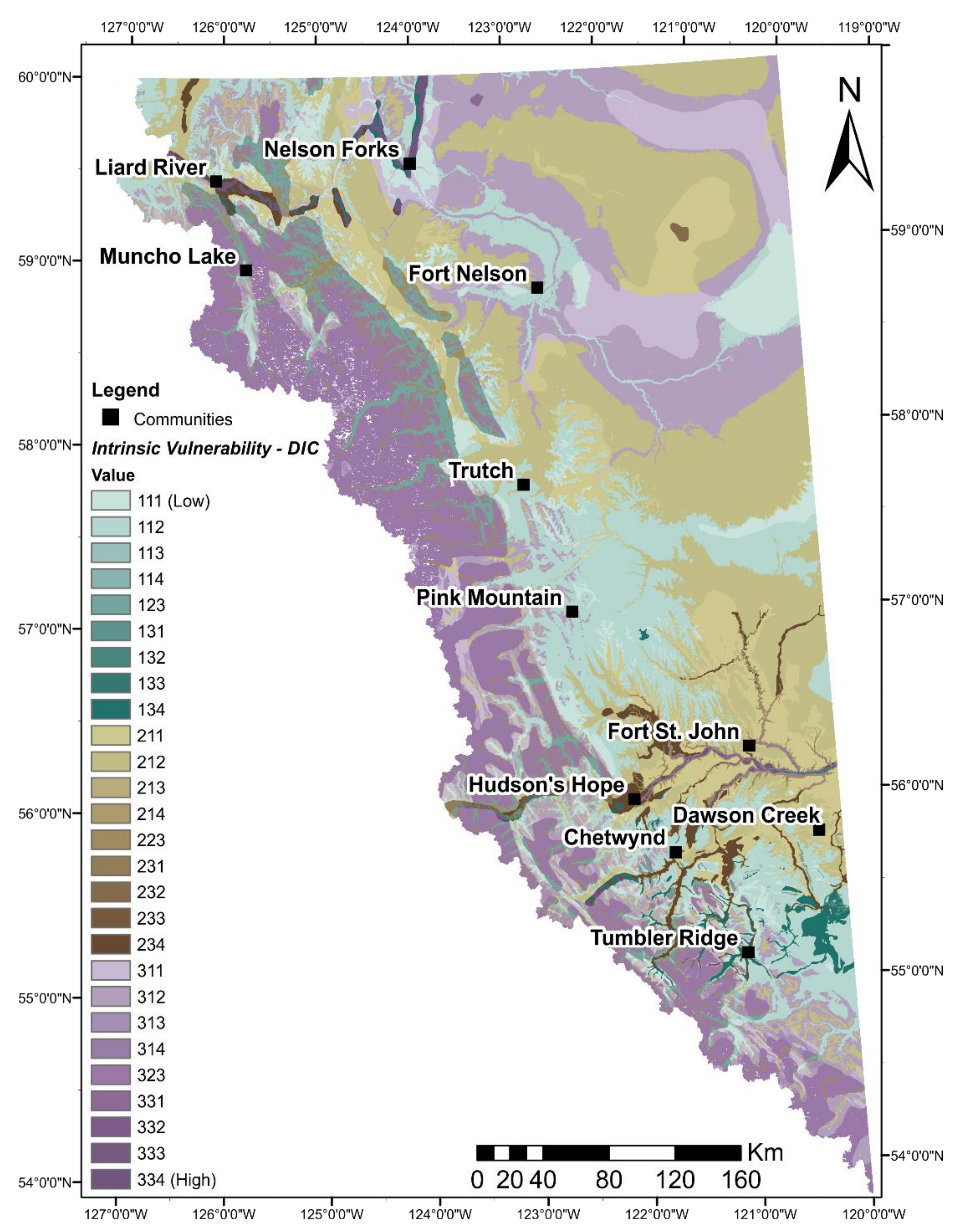
The D-I-C intrinsic vulnerability map (
Figure 1) was constructed by combining the three factors using the GIS raster calculation tool. The final output raster was a combination of three numbers that represent the D-I-C factors: for example, 1-1-2, representing D = 1 (water table depth range 24–30 mbgs), I = 1 (glaciolacutrine sediments forming the vadose zone), and C = 2 (glaciolacustrine sediments in the saturated zone). The legend in
Figure 1 lists the factor combinations according to their relative intrinsic vulnerability to contamination from the surface.
The different ranks of each factor resulted in 36 combinations, although only 27 combinations (scenarios) were considered, as some of the scenarios were unrealistic because they represent bedrock on top of Quaternary sediments.
2.3. Numerical Modelling
2.3.1. Model Setup
A series of 3D density-dependent flow and transport simulations were run using the TOUGH2 code, a simulator for non-isothermal multiphase flow in porous media [
24]. TOUGH2 calculates the thermophysical properties of fluids through different equation-of-state (EOS) modules. For this study, the EOS7 module was used to describe multiphase mixtures of water, brine, and air with density and viscosity effects in both the gas and liquid phase [
30].
A typical site in NEBC was conceptualized as a 200 m by 200 m base box model, 30 m deep. The base box model is defined as a quadrant of the full, tridimensional box model gridded as 400 m × 400 m × 30 m (
Figure 2). The purpose of having a ¼ size base box model was to reduce the computational time. An edge distance of 200 m was selected to allow for ample space for the plume to travel. This distance is comparable to the 100 m distance threshold stated in the
BC Oil and Gas Activities Act, which is related to the closest a well [oil and gas] can be to a natural boundary of a water body [
31]. The 30-m depth of the model was based on knowledge that the bedrock surface throughout the area is largely within 30 m of ground surface [
18].
It was assumed there was no flow across the boundaries of the model; thus, all the model edges were set to no flow (zero flux) except for the injection cells, which were used to represent the spills or leaks. The simulations were set to run for 10 years with no regional flow or recharge. Overall, 27 model scenarios were constructed to represent the range of combinations of D-I-C factors and ranks (
Table 1). Additional simulations examined the effect of regional flow on WW transport. For these regional flow models, full box models were used with injection at the centre. A sensitivity analysis was also performed to explore the effect of changing different model parameters including permeability, porosity, and capillary pressure values, as well as the volume and injection rate of the WW fluid. Details regarding the regional model setup and the sensitivity analysis, along with the results, are provided by Rosales-Ramirez [
32]. This paper focuses primarily on spills and the results of the ¼ base box models, because the modelling results were used to construct the specific vulnerability maps.
Model domains were constructed with three layers representing the unsaturated zone (Layer 1 = L1), a saturated zone (Layer 2 = L2), and bedrock (Layer 3 = L3) (
Figure 2). The thicknesses used for L1 were based on the ranks for Factor D, using the median value of the range of depth to water table (
Table 1); thus, these measurements represent the vadose (henceforth unsaturated) zone thickness. The discretization in the Z direction was 30 cells of 1 m thickness each. Consequently, the number of cells varied within L1 and L2 depending on the thickness of the unsaturated zone. For example, for a depth to the water table of 27 m, the discretization of L1 was 27 cells, for L2 it was 2 cells, and for L3 it was 1 cell. Laterally, the grid was refined closer to the injection cells (
Figure 2). In preliminary modelling, the extent of the spill was found to be contained within the first ~105 m from the injection area; thus, a coarser grid was assigned after 100 m to improve computational time.
Permeability and porosity values for the different material types, representing Factors I and C, are given in
Appendix B (
Table A1). Values are based on the literature ranges for the material types found in NEBC [
28,
29]. Permeabilities in the Z direction were assigned values one order of magnitude lower than in the X-Y directions [
33].
The models involved the flow of two immiscible fluids (water and air) in the unsaturated zone; therefore, capillary pressure (Cp) and relative permeability (Rp) relationships were taken as a function of fluid saturation [
24].
Appendix B shows the van Genuchten [
34] equations and associated curve fitting parameters (
Table A2) that were summarized from experimental results reported in the literature [
35,
36,
37,
38,
39,
40,
41]. In this study, the van Genuchten–Mualem model [
42] was used to calculate Rp.
2.3.2. Spill Volume
There are more than 44,500 km of pipelines in NEBC regulated by the BCOGC [
43]. The majority of these pipelines are buried, and currently, over 39,000 km are operating and transporting refined or unrefined products, such as sour natural gas, natural gas, crude oil, and water (freshwater, produced water, saltwater, and sour water), among other products. Spill volume estimates for this study were based on the pipeline performance reports and the spill incident map from BCOGC [
44]; it should be noted that the incident map does not show incidents prior to 2009. The BCOGC defines an incident as an event resulting from oil and gas activities outside of normal operations, which may or not be an emergency. Particularly, a “spill” is the unauthorized release or discharge of a substance into the environment. In the case of produced/saltwater, a permit holder must report the incident to the BCOGC if the spill is equal to or greater to 200 kg or 200 L, or if it impacts waterways [
45].
A total of 1675 incidents were reported from 2000 to 2018, with 916 liquid spill or leakage incidents and 270 events identifying the product release as produced/saltwater (17 events reported the product as unknown), although early data from 2000–2006 could also include produced/saltwater as a miscellaneous liquids release. Overall, the incident reports showed limited information regarding spills from 2004 to 2018. The registered volume of liquid discharge was sparsely reported (or not reported), but varied between 0.03 and 4000 m
3 (see [
32] for a listing of all reported spills and spill volumes from 2004 to 2018). Data on the extent of a spill were not provided in the majority of the incidents, except for a few events reporting covering areas between 3 and 200 m
2. Some incidents were reported to be less than 200 m away from surface water bodies (one incident reported the drilling location 32 m away from a river), although winter conditions resulted in the fluid spill freezing, facilitating the cleaning and remediation procedures. The BCOGC Incident Map does not include non-BCOGC regulated pipelines and National Energy Board (NEB)-regulated pipelines. The NEB reported 256 incidents in B.C. from 2008 to 2018 (June), with only one incident identified as a 20 m
3 produced water spill, which occurred in 2015 [
46]. Based on the reported spill incidents, the median volume of a fluid spill (mostly produced water) in NEBC was 10,000 L.
In TOUGH2, sources and sinks are used to define the flow in a cell (in or out) by specifying the time and rate of injection of a defined fluid. For these models, the injected fluid is brine, which is similar to the high-density WW. To represent the fluid release of WW in the models, a spill was simulated using 16 injection cells (4 by 4 cells), in the top left corner of the model when viewed in cross-section (
Figure 2), with a size of 1.25 m by 1.25 m in the X-Y axis and 1 m in the Z direction. In total, 16 cells were used for injection, covering a total area of 25 m
2 with a volume of 20 m
3.
The brine was modeled as a NaCl solution and the brine density was adjusted according to the total dissolved solids (TDS) values reported for flowback water from 24 wells, completed in the Montney Formation. The TDS values ranged between 24,000 and 228,000 mg/L, with mostly Cl and Na composition [
47]. For the models, the brine density was set to 1208.5 kg/m
3, reflecting a TDS value of ~230,000 mg/L. The reference temperature was 25 °C and the reference pressure 1.013 × 10
5 Pa. The effects of salinity on density, viscosity, and gas solubility are accounted for in the EOS7 module of TOUGH2 [
24].
Consistent with the median reported spill volume, a 10,000 L volume was injected over 15 days at a rate of 50.4 kg/day per injection cell to simulate a spill.
2.3.3. Initial Conditions and Solver Settings
Initial pressure distributions were obtained by performing a series of preliminary TOUGH2 runs. The first run used single-phase conditions for the entire model and a temperature of 6.5 °C, based on the average groundwater temperatures measured in samples in NEBC [
18], and a default pressure of 1.013 × 10
5 Pa. Thereafter, the pressures for each cell obtained from this initial run were used as the initial conditions. The subsequent run was used to establish the unsaturated zone conditions, where L1 was designated as two-phase with an initial gas saturation of 0.80. The final run provided the correct pressure distribution (air and water) for the model under saturated and unsaturated conditions as well as the unsaturated zone gas saturation; these were used as the initial conditions for the 10 years simulation. This approach of pressure estimation was performed for all models before the injection cells were added. The biconjugate gradient solver was used for all simulations; the various solver settings are provided in
Table A3.
3. Results
3.1. Transport Simulations
Overall, the modelling results showed that WW plumes travel vertically downward to the water table and begin to spread laterally when they reach a lower permeability basal layer. Plumes within highly permeable materials travel faster and migrate further, while in low permeability materials, the migration rate is slower. For example, the model scenario characterized by glaciofluvial materials in the unsaturated and saturated zone, and for the shallowest water table (scenario 3-3-4), showed the WW traveling rapidly in the unsaturated zone with almost no radial spreading until reaching the basal low permeability material at 30 m, with a plume extent of ~24 m after 10 years (
Figure 3). After the fluid was injected, the plume reached the saturated zone in ~60 days and the bottom of the aquifer at approximately 4.5 years, where it continued to spread radially. There was some lateral migration at the base of the unsaturated zone and in the middle to upper portion of the saturated zone; however, this tended to diminish over time as the downward directed flux dominated in these regions. The rest of the models categorized as Rank 3 for Factor D, but with different aquifer materials (models 3-3-3, 3-3-2, and 3-3-1), showed a similar behavior as model 3-3-4 regarding the WW footprint.
In the scenarios with highly permeable material in the unsaturated zone and lower permeability material in the saturated zone, lateral migration dominated and there was no appreciable penetration into the saturated zone.
Figure 4 shows an example for the unsaturated zone comprised of glaciofluvial sediments overlying a sandstone aquifer.
The regional flow models showed that the presence of a head gradient results in greater lateral migration rates, enhancing the plume footprint in the direction of the regional flow. As the gradient increased, the WW plumes were longer and narrower compared to the zero gradient models. Simulation results for all combinations of D-I-C factors and the regional models are described in detail by Rosales-Ramirez [
32].
3.2. Plume Travel Times
The scenarios with depth to the water table of 12 m (Rank 3 for Factor D) and an unsaturated zone characterized by glaciofluvial materials (Rank 3 for Factor I) showed the fastest travel times during the simulations (
Figure 5). The highest velocities were encountered within the unsaturated zone where there was a higher gravity force. As the plume moved from the injection area towards the edges of the model, the plume slowed. In some models, the WW did not reach the saturated zone during the 10-year simulation, particularly in those models with a depth to water table of 21 and 27 m (Rank 2 and Rank 1 for Factor D, respectively) and characterized by an unsaturated zone comprised of sandstone or glaciolacustrine/till material (Rank 2 and Rank 1 for Factor I, respectively).
As seen in
Figure 5, there was a trend in the models characterized by Rank 3 for Factor I (unsaturated zone characterized by glaciofluvial materials) clustering near the 0 year mark and showing faster migration rates, while the models of Rank 2 and Rank 1 for Factor I (unsaturated zone characterized by sandstone and glaciolacustrine materials, respectively) showed longer travel times to water table. Thus, regardless of the depth to water table, the material characterizing the unsaturated zone appeared to be the primary control on the plume migration rates.
In models with Factor D and Factor I, both of Rank 3, the WW reached the water table in less than 90 days, with the WW in model 3-3-4 reaching the water table between 60 and 70 days. The combination of a shallow water table and glaciofluvial material in the unsaturated zone resulted in the fastest travel times to reach the water table. Based on plume migration to the water table (12 m), rates were estimated between 48.6 and 73 m/year. Although, by the end of the simulation, the velocities were dramatically reduced (~1 × 10⁻² m/year), reflecting how the driving forces decrease over time as the plume migrates. Velocities through the unsaturated zone where the water table was at 21 m were approximately 29.5 m/year, and for the 27 m water table they were approximately 18 m/year. The slowing of the migration rate reflects the diminishing driving force as brine becomes residually trapped in the pore space of the unsaturated zone and reduces the mass of water that is able to flow.
In models characterized by Rank 3 for Factor D (12 m depth) and Ranks 2 and 1 (sandstone and glaciolacustrine/till, respectively) for Factor I, the WW did not reach the water table during the 10-year simulation (outside the red areas in
Figure 5). Thus, for these models, the low permeability of the unsaturated material completely controlled the migration rate of the plumes. Using the vertical distances travelled during the 10-year simulation, it was estimated that in these models the WW could take thousands of years to reach the water table depending on the unsaturated zone material. However, these estimates were not based on modelling for the entire time frame. It was expected that, in longer-term models, the brine would remain as residual water in the unsaturated zone and there would be no driving force to promote migration.
In general, most of the models showed fluid velocities decreasing as the plume reached the water table, particularly in models where there were different materials characterizing the unsaturated and saturated zone. In addition, migration rates tended to be slower beneath the water table, because once the WW enters the aquifer, there is less density contrast between the brine and the water in comparison with the unsaturated zone (brine/air). As was observed, the WW migration rate and direction depend on the material characterizing each zone; thus, permeability is mostly governing the fluid behavior. Moreover, the material comprising the unsaturated zone regulates the rate at which the brine is entering the aquifer. Materials characterized by high permeability showed the highest velocities in comparison with materials of low permeability, which had the lowest velocities.
3.3. Plume Travel Distances
The plume distance refers to the total distance migrated in the saturated zone in the X-Y and the Z directions. In some scenarios, the plume did not reach the saturated zone within the 10-year simulation, particularly in models with an unsaturated zone characterized by low permeability materials (
Figure 6, models at 0 m). The longest plume distances in the X-Y direction were encountered in the models characterized by a glaciofluvial unsaturated zone for any depth to water table; and similar results were observed in the Z direction (results not shown). However, in all directions, a shallower water table also influenced some of the modelling results.
Beginning with the radial distance (
Figure 6), similar behavior was observed in models with the unsaturated zone comprised of glaciofluvial materials (Rank 3 for Factor I). As the WW is moving downward, the unsaturated zone below the spill/leak becomes more saturated. When the brine reaches the water table it either continues to migrate downward, if the aquifer is permeable, or migrates laterally. Once the plume reaches the water table interface, the difference in permeability due to the lower permeability aquifer material causes the plume to spread along in the X-Y direction. Thus, a shallow water table promotes longer radial distances versus a deeper water table. Overall, the WW plume migrated laterally between 10 m and ~24 m. Thus, these models recorded the longest radial distance during the 10-year simulation regardless of the depth to water table.
As seen in
Figure 6 (first four models in color purple), the longest distances recorded were for the models characterized by glaciofluvial materials in the unsaturated zone for a 12 m water table depth. In these models, the brine flows down faster through the glaciofluvial materials until it reaches the saturated zone or a low permeability material where it sits and spreads laterally (see
Figure 3). After 10 years, the radial distances in these models ranged between 23.5 and 24.5 m, followed by models with a 21 m depth to water table (brown models in
Figure 6) with radial distances ranging from 12.3 to 16.6 m; and lastly, models with a deep water table reached radial distances between ~10 and 12 m. In general, the radial extent reduces as the water table depth increases. Finally, in the models where the WW did not reach the saturated zone, both the saturated and unsaturated zone had low permeability materials, which promote lower migration rates through the unsaturated zone. Thus, the plume’s footprint is shorter and does not reach the water table.
3.4. Plume Concentrations
In all of the models, the brine concentration decreased as the plume migrated from the injection area. Higher brine concentrations occurred downgradient in areas adjacent to the spill/leak source (injection cells) and mostly on top of the water table. The models displayed similar behavior in the plume concentration, depending on the material characterizing the unsaturated zone at any water table depth. As soon as the plume entered the saturated zone, the concentrations rapidly decreased because of dilution.
High brine concentrations in models with Rank 3 for Factor I (glaciofluvial materials in the unsaturated) were found mostly within the area below the injection cells and above the water table. In general, during early times after the injection period, the plume had a brine concentration between 1.00 and 0.90 within the first 3 mbgs, whereas in the X-Y direction, these high concentrations extended up to ~4.5 m. As the brine approaches the saturated zone, the concentrations begin to dilute because of mixing with the residual water in the unsaturated zone pore space. At 10 years, the highest concentrations were found within the unsaturated zone below the injection cells extending 4.8 m radially, whereas in the saturated zone, the concentrations were appreciably lower, ranging from 0.1 to 0.00001. Similar concentration patterns were observed in models with a glaciofluvial unsaturated zone at any depth to water table. Thus, in
Figure 7 it can be observed that for a deep water table (i.e., models 2-3-4 and 1-3-4), the plume travels a longer distance; thus, there is a larger area with high brine concentration in the models with a 21 and 27 m depth to water table. As the brine migrates through glaciofluvial materials in the unsaturated zone, it becomes quickly saturated, whereas in the saturated zone, the brine rapidly dilutes. Overall, in these models after 10 years of simulation, elevated brine concentrations were found only within the unsaturated zone, and gradually decreased as the plume migrated down and laterally.
Models with an unsaturated zone comprised of bedrock and glaciolacustrine/till materials displayed similar plume footprints and concentration distributions. As low permeability materials define the unsaturated zone, the highest concentrations were found within this area, in smaller footprints and mostly lateral spreading.
The combination of a low permeability layer and the unsaturated environment promoted lower migrations rates and favored transport in the X-Y direction. Within the unsaturated zone, there was a residual water content (average 20% of porosity); hence, lower concentrations occurred through dilution. Therefore, the highest concentrations in the models were encountered closest to the injection site.
Generally, the lower concentrations along the edges of the plume are due to dispersion and dilution occurring in the saturated zone. Although TOUGH2 does not explicitly account for hydrodynamic dispersion, the code produces a certain amount of numerical dispersion dependent on velocity. The aquifer thickness is also a factor that determines the ability and rate for the groundwater to dilute the brine plume. A thicker aquifer allows for more dilution, resulting in lower concentrations in comparison with a thinner aquifer. In addition, it was expected that once the injected brine in the unsaturated zone was exhausted, the plumes would keep on spreading, leading to an even greater decrease in concentration and larger footprint.
Lastly, it was found that after 10 years, a large proportion of the injected brine and high brine concentrations were present within the unsaturated zone despite the material or depth to water table. As mentioned above, as the driving forces diminish during plume migration, some brine is left behind, filling the pore space. The residual brine remains present in this volume unless a recharge by precipitation is taking place. In this study, recharge was not modelled, but it is expected to increase the vertical migration of the WW, particularly through the unsaturated zone. High recharge rates likely dilute and transport the remaining brine down through the unsaturated zone, posing a longer-term threat of water quality deterioration.
4. Discussion
The vulnerability maps were constructed on the basis of the modelling results and are presented as a series of specific vulnerability maps. Areas highly vulnerable to water quality deterioration from a WW spill can be seen in all maps (
Figure 8,
Figure 9 and
Figure 10), specifically in the areas around Dawson Creek, Chetwynd, and Fort St. John, as well as a small area in the northwest close to Nelson Forks.
Figure 8 shows the travel time to reach the water table. The high vulnerability areas are river valleys characterized by sand and gravel materials in both the unsaturated and saturated zones with shallow water tables. In these areas, the WW reached the water table in less than 1 year of simulation (
Figure 8).
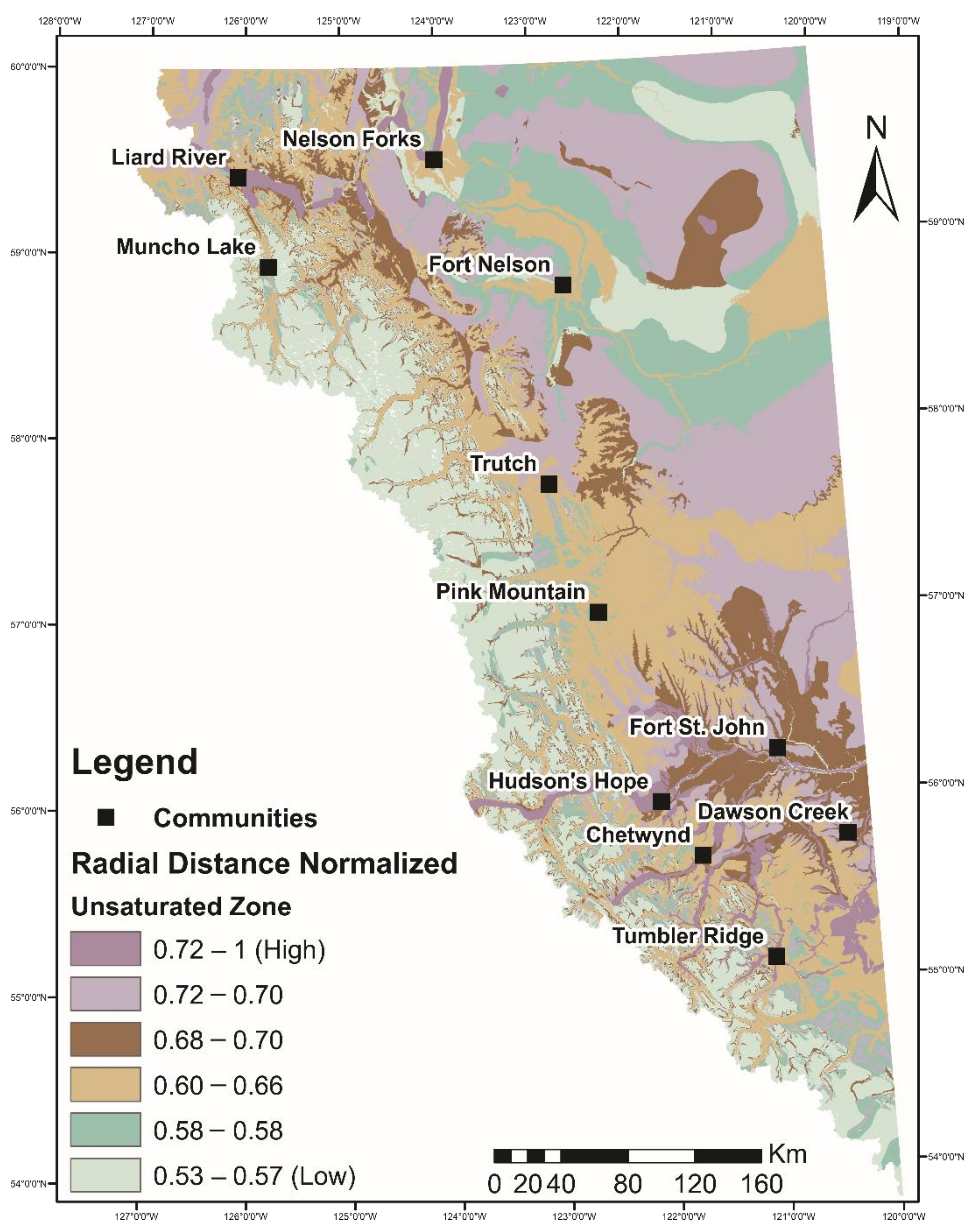
Figure 9 and
Figure 10 show the distances reached during the 10-year simulation in the unsaturated zone for the “X-Y” (radial) and “Z” (vertical) directions, respectively. Normalized distances are shown on these maps, which is the distance reached as a proportion of the maximum distance reached during the 10-year simulation period. Normalized distances are used to give an indication of the relative vulnerability of the different model scenarios. For example, in
Figure 9, the maximum radial distance reached was 7.5 m at the end of the 10-year simulation period, while in
Figure 10, the maximum vertical depth reached was 27 m.
Vulnerability to radial plume migration in the unsaturated zone ranged from the lowest values of 0.53 to the highest values of 1 (
Figure 9). The least vulnerable are areas characterized by till or glaciolacustrine materials (teal-colored areas), which promote slower migration rates. On the other hand, in the Z direction it can be observed that most areas have low vulnerability as a result of the plume not reaching the water table within the 10-year simulation (
Figure 10). Longer vertical distances were only simulated in areas characterized by high permeability materials, which allow for faster migration rates despite the depth to water table. Overall, vertical migration is faster than radial migration because gravitational driving forces influence the WW.
Maps illustrating distances reached during the 10-year simulation period in the saturated zone (both radial and vertical) are not shown because the distances are very short, except in the more permeable sediments found in river valleys. As mentioned above, once the plume enters the saturated zone the migration and plume footprint are controlled by the permeability of the materials. Thus, in the saturated zone, the longest distances reached correspond to glaciofluvial materials in comparison with the short ones from glaciolacustrine materials. As expected, the vulnerability in the saturated zone is closely related to the permeability characterizing the unsaturated zone, which controls whether the WW reaches the saturated zone and continues to migrate radially.
In areas characterized by a vadose zone consisting of fractured bedrock (Rank 2 for Factor I), the simulations suggest that the WW plume will not reach the water table within 10 years, even when combined with a shallow water table (
Figure 5). However, these models might underestimate the vulnerability in these areas, because they simulate flow and transport through a porous medium. It is expected that fractures lead to faster migration rates.
Overall, across NEBC, the distribution of materials in the subsurface is poorly constrained; however, if there is a shallow water table with till overlying a sand and gravel aquifer, then there is potential for the brine to migrate into those aquifers and redistribute, especially if recharge or other driving forces are present. The low permeability materials in the unsaturated zone promote slower migration rates, and local higher brine concentrations; thus, groundwater quality deterioration is low in these areas. Moreover, much of the region is characterized by deeper water tables; hence, there is a lower potential for the brine to migrate to those greater depths. Ultimately, the most vulnerable areas are a result of the combination of highly permeable materials characterizing the unsaturated and saturated zones, resulting in faster migration rates in all directions (purple areas in all maps).
The results of this study are generally consistent with generic spill scenario modelling, which is aimed at identifying whether produced water-release scenarios (i.e., WW-release scenarios) may impair groundwater [
12]. In the study by the authors of [
12], the model scenarios differed from this study in terms of (1) the modelling software used (as mentioned earlier, that study did not consider the effects of density-dependent flow on the transport of brine); (2) slightly lower brine concentrations (100,000 ppm vs. more than twice that in this study-230,000 mg/L); (3) much larger spills (up to 1.6 × 10
6 L vs. 1 × 10
4 L in this study); and (4) representation of the surface spills (surface thickness vs. injection rate in this study). Despite these differences in model setup, the main outcomes are the same, namely that shallow depth to water table and high permeability substrates are dominant controls on travel times, distance travelled, and concentrations.
5. Conclusions
This study identified the physical controls dominating the flow and transport of a WW spill in the shallow subsurface zone. The type of material, and hence, its permeability, influences the WW footprint (radial and vertical extent). Accordingly, the NEBC vulnerability maps show the areas that are most susceptible to water quality deterioration from a WW spill. These maps were provided to the BCOGC as a decision-making tool to reduce the risk of potential groundwater contamination and improve the understanding of vulnerable areas, as well as to raise awareness and promote better monitoring and spill mitigation practices. A major finding of this research is that the combination of a high-impact vadose zone rating (Factor “I”) and the conductivity of the aquifer material rating (Factor C) increased the vulnerability to water quality deterioration in the shallow subsurface.
Figure 11 shows that across NEBC there are a large number of pipelines (~6400 km) operating near high vulnerability areas. It is estimated that ~1.5% of the current active and new pipelines are located within high vulnerability areas, and that ~5% are within moderate vulnerability areas. Furthermore, spills can also occur during transportation or on/near the well pad. It was assessed that ~50 km
2 of roads (permitted) are in areas of high to moderate vulnerability, while ~8% of the current oil and gas wells and facilities in NEBC are in moderate to high vulnerability areas. Of particular interest are the areas near communities like Dawson Creek, Hudson Hope, and Fort St. John, where most of the aquifers are unconfined and characterized by sand and gravel materials (
Figure 11). In these areas, a WW spill can reach the saturated zone most rapidly, hence the need for constant monitoring and faster spill response protocols.
Although spills cannot be predicted, their impacts can be greatly reduced and perhaps even prevented by enforcing regulations and enhancing monitoring practices, particularly where pipelines or roads and moderate to high vulnerability regions intersect. This research does not account for or fully predict the degree to which an aquifer can be contaminated; however, the vulnerability maps can be used as a preliminary risk assessment tool, as they are based on the main factors influencing the potential of a WW spill to contaminate an aquifer.
The models in this study were developed using the current available data; however, because shale gas and other petroleum development is ongoing in NEBC, new available data can easily be incorporated within the groundwater vulnerability method. At that point, the D-I-C parameters, the numerical models, and thus, the vulnerability maps, can be updated and refined. The advantage of the groundwater vulnerability method combined with the D-I-C—numerical modelling approach is that the methodology is not area specific, which allows for modification and adaptations to other study areas with current or future shale gas development.


