Identification of Road Traffic Injury Risk Prone Area Using Environmental Factors by Machine Learning Classification in Nonthaburi, Thailand

Abstract

Road traffic injuries are a major cause of morbidity and mortality worldwide and currently rank ninth globally among the leading causes of disease burden regarding disability-adjusted life years lost. Nonthaburi and Pathum Thani are parts of the greater Bangkok metropolitan area, and the road traffic injury rate is very high in these areas. This study aimed to identify the environmental factors affecting road traffic injury risk prone areas and classify road traffic injuries from an environmental factor dataset using machine learning algorithms. Road traffic injury risk prone areas were set as the dependent variables for the analysis, with other factors that influence road traffic injury risk prone areas being set as independent variables. A total of 20 environmental factors were selected from the spatial datasets. Then, machine learning algorithms were applied using a grid search. The first experiment from 2017 in Nonthaburi and Pathum Thani was used for training the model, and then, 2018 data from Nonthaburi and Pathum Thani were used for validation. The second experiment used 2018 Nonthaburi data for the training, and 2018 Pathum Thani data were used for the validation. The important factors were grocery stores, convenience stores, electronics stores, drugstores, schools, gas stations, restaurants, supermarkets, and road geometrics, with length being the most critical factor that influenced the road traffic injury risk prone model. The first and second experiments in a random forest model provided the best model environmental factors affecting road traffic injury risk prone areas, and machine learning can classify such road traffic injuries.

1. Introduction

According to the World Health Organization (WHO), 1.2 million people die because of road traffic collisions every year. On average, 3242 people are killed daily. Approximately, 20–50 million people are injured or disabled in traffic collisions. Furthermore, road traffic injuries are a leading cause of death among young people (15–19 years of age). Approximately, 90% of road traffic deaths occur in low- and middle-income countries [1].

Road traffic injuries are a major cause of morbidity and mortality worldwide, especially in low- and middle-income countries, and they currently ranks ninth globally among the leading causes of disease burden regarding disability-adjusted life years lost.

Studies have shown that road traffic accidents (RTAs) have complicated consequences, which are caused by human, vehicle, and environmental factors. The impact of the environmental factors, in terms of road traffic accidents, has been of interest to researchers for a long time. Researchers are interested in weather/seasonal effects on road traffic injuries. Jones et al. [2] studied the influence of geographical variations on RTAs and found a significant association between rainy and foggy days with an increase in the number of road traffic accidents, while some researchers are interested in the influence of lighting conditions on road traffic injuries. Light conditions can be affected by mist and dewdrops that noticeably and continuously fluctuate around the environment. Lam et al. [3] focused on the impacts of light on pedestrian-related accidental cases. In addition, some researchers are interested in the point of interest (POI) that affects road traffic accidents. Jia et al. [4] studied a spatial clustering method for macro-level traffic crash analysis based on open-source POI data and traffic crashes. They found that residential density, bank, and hospital POIs have significant positive impacts on traffic crashes, whereas stores, restaurants, and entertainment venues are found to be irrelevant for traffic crashes. Therefore, environmental factors have great importance due to their effects on traffic accident severity and their injuries. More importantly, some of these factors are controllable by addressing engineering and track designing problems.

For many years, identifying hotspots and traditional statistical modeling have been standard methods for finding the causes of road traffic injuries. Identifying the hotspots of road traffic injuries is an important factor for detecting risk-prone areas. Hotspot detection techniques, such as Getis-Ord Gi*, local Moran’s I, and kernel density estimation, have been used to investigate the impacts of accidents [5,6]. Moreover, the spatial correlations between crash occurrence and the spatial dependence of crashes have also been investigated [7]. Ulak et al. [7] compared the accuracy and performance of hotspot delineation using different hotspot detection techniques (Getis-Ord Gi*, local Moran’s I, KLINCS (K-function local indicators of network-constrained clusters), and KLINCS-IC (Inverse Cost)) under different roadway network-based spatial weights. Several similar research projects have been conducted for hotspot analysis comparison purposes [8]. Several types of research have examined the correlation between behavior and location. Bil et al. [9] studied the spatiotemporal expression of a hotspot by using the kernel density estimation (KDE)+ from crash data over 3 years, as did Liu and Sharma [10].

Hotspot analysis is case-based and requires a road traffic injury dataset to analyze the hotspot. This method does not indicate factors influencing road traffic injuries and is not applicable if road traffic injuries data are not available.

Over the last decade, traditional statistical techniques have been implemented to study the relationship between road severity and influencing factors. Yan et al. [11] illustrated that seven road environment factors (number of lanes, divided/undivided highway, accident time, road surface condition, highway character, urban/rural, and speed limit), five factors related to prominent roles (vehicle type, driver’s age, alcohol/drug use, driver’s residence, and gender), and four factors related to struck roles (vehicle type, driver’s age, driver’s residence, and gender) are significantly associated with the risk of rear-end accidents. Furthermore, a significant interaction effect was observed among those risk factors when analyzed with logistic regression. Karacasu et al. [12] showed that vehicle type, purpose, education level, seat belts, and traffic signs are related to traffic accidents. However, different road accident severities depend on the independent variable, which means risk-prone areas depend on their environment.

Traditional statistical techniques are based on parametric assumptions and are useful in finding relationships between variables and the significance of those relationships. Machine learning algorithms can learn from the data without relying on rule-based programming. To overcome the limitation of traditional statistical techniques, nonparametric methods and artificial intelligence models have been used in different domains, including traffic accidents. Yeoum and Lee [13] developed an accident prediction model to predict the chance of accident occurrences for the Republic of Korea Air Force using an artificial neural network (ANN) and logistic regression analysis. Aircraft accident records for 30 years were used during the analysis and revealed that 9 out of 13 selected variables influence these incidents. Machine learning and artificial intelligence are also becoming popular in other domains, such as hydrology [14] and the construction industry [15].

In the context of traffic accidents, many researchers have tried to improve accuracy by focusing on area and population techniques. For instance, Elvik et al. [16] focused on a road bridge in Norway, and Yang et al. [17] attempted to study two-wheel electric vehicle drivers at intersections. However, these techniques are limited to a small dataset, and a detailed analysis of factors associated with accidents is recommended. In Thailand, there remains a scarcity of studies on the prediction of road traffic injuries with a large dataset. The assessment and prediction of road traffic injuries in risk-prone areas is now a necessity to reduce these incidents.

Spatial prediction of road traffic injuries in risk-prone areas is a crucial step for road traffic injury hazard mitigation and management. The spatial probability of road traffic injuries in risk-prone areas can be expressed as the probability of spatial occurrence of a set of environmental conditions. Producing a reliable spatial prediction of road traffic injuries in risk-prone areas is not possible. For this reason, various approaches have been proposed in the literature.

The ability to solve nonlinear problems makes machine learning algorithms applicable to traffic accident analysis. Chong et al. [18] summarized the performance of four machine learning paradigms applied to model the severity of the injuries that occur during traffic accidents. Experimental results revealed that among the machine learning paradigms considered, a hybrid decision tree-neural network approach outperformed the individual approaches. Rahman et al. [19] evaluated the machine learning techniques to analyze pedestrian and bicycle crashes at a macro-level. A gradient boosting method outperformed other competing traditional techniques for macro-level crash prediction models. Similarly, Kashani et al. [20] studied the injury severity of pillion passengers in Iran over four years.

Moreover, machine learning algorithms can learn from a large training dataset at a fast learning rate. Arhin and Gatiba [21] implemented support vector machines (SVMs) and Gaussian naïve Bayes classifiers (GNBCs) to predict the injury severity of crashes. A total of 3307 crashes that occurred from 2008 to 2015 were used to develop the models (eight SVM models and a GNBC model). The SVM model based on the radial basis kernel function was found to be the most accurate model. This model was able to predict accident-related injury severity with an accuracy of approximately 83.2%. GNBC showed the lowest classification accuracy of 48.5%.

In this study, there are two research questions: (1) Can machine learning predict road traffic injuries in the same study area but for different years? (2). Can machine learning of a road traffic injury model for the Nonthaburi area predict road traffic injuries in the Pathum Thani area?

This paper is structured as follows: Section 2 provides information about the study area: Nonthaburi and Pathum Thani, both of which are developing areas near Bangkok with frequent road traffic accidents. This section describes the datasets that are used for analysis. Section 3 details the experiments and results. The overall methodology of the research is described in Section 4, which provides a discussion, conclusions of the research, and recommendations for further improvement. Recommendations for policymakers are also included.

2. Data and Methods

2.1. Case Study

Two developing provinces of Thailand, Nonthaburi and Pathum Thani, were selected for this research. Both provinces are adjacent to Bangkok, the economic center of Thailand, and are secondary areas of the city.

Nonthaburi has two city municipalities, seven town municipalities, and eleven subdistrict municipalities. Pathum Thani has one city municipality, nine town municipalities, and seventeen subdistrict municipalities. Nonthaburi is a densely populated city, whereas Pathum Thani is a densely industrial city. As of 2017, the human achievement index of Nonthaburi and Pathum Thani was 0.68 and 0.64, respectively.

Nonthaburi and Pathum Thani comprise part of the greater Bangkok metropolitan area. They incur a high number of road traffic injuries. Road traffic injuries occur in places of cities where residential, industrial, and commercial areas are located. These areas are the focus of all kinds of human activities, providing economic opportunities to their inhabitants, which attract the rural population in mass. In these urban areas, a large proportion of people, including migrants from rural areas, commute every day using different modes of transportation, exposing them to the risk of road traffic injuries.

2.2. Data

To analyze the correlation between environmental factors and road traffic injury risk prone areas, the road traffic injury risk prone areas were set as dependent variables, and other factors that influence those road traffic injury risk prone areas were set as independent variables. A total of 20 environmental factors were considered from the spatial datasets. Road traffic injuries datasets obtained from 2017 and 2018 were used for the training and validation, respectively. The factors from the maps were resampled into a 50 m × 50 m grid format using the FISHNET tool in QGIS. 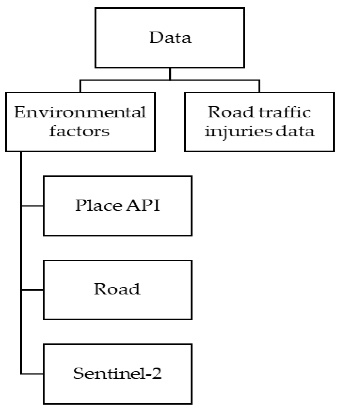Figure 1 shows data of this study.

2.2.1. Environmental Factors

It is not easy to obtain accurate and reliable dataset from the government. This is an obstacle to spatial data analysis. However, with the help of open-source data, the data at the point of interest are reliable. POIs can be collected from many sources. However, they may not be a common factor used to analyze traditional road traffic injuries. Nevertheless, these POI data are specifics of land use factors with accurate location data that are expected to be related to users’ characteristics and road traffic injuries.

Due to the fact that traffic volume data do not include historical data in the year required, the study focused on POI-based spatial data analysis, including a road dataset and satellite index. The POI data were included with road traffic injury data later. The advantage of POI data is that the data precisely represent land use, which leads to precise solutions. The environmental factors were collected from three sources: Place Application Programming Interface (Place API), the road, and Sentinel-2. Place Application Programming Interface (Place API) Current open-source data provide precise location intelligence and comprehensive location data. For this study, the environmental factors affecting road traffic accidents and the set of environmental factors derived from the point of interest were used as input factors for machine learning algorithms to predict road traffic accident injuries. For the analysis, a dataset of twenty explanatory variables was derived from a web map service. The variables include grocery stores, convenience stores, home goods stores, food stores, clothing stores, electronics stores, furniture stores, car repair shops, clothing stores, hardware stores, health care facilities, pet stores, bicycle stores, electronic repair shops, drugstores, supermarkets, shoe stores, schools, gas stations, and restaurants.

Each explanatory variable was reclassified using standard deviation. All of the reclassified variables were then converted to a 50 m × 50 m grid format using a spatial joins operation.

Road

Although the study focused on POI data, common factors were also used to analyze traditional road traffic injuries, such as length and road data intersection.

A road dataset was obtained from the Nonthaburi office of public works and town and country planning. Two explanatory variables, length, and intersection were derived from the road dataset. Each explanatory variable was reclassified using standard deviation and then converted into a 50 m × 50 m grid format using a spatial joins operation.

Sentinel-2

The normalized difference built-up index (NDBI) has been useful for mapping urban built-up areas. Sentinel-2 satellite images covering the study area on 27 April 2017 were downloaded, and the NDBI was extracted. The NDBI raster was also reclassified and reprojected to a 50 m pixel size.

Descriptive statistics of the independent variables of Nonthaburi and Pathum Thani Provinces are given in

Table 1. Characteristic parameters of the road environment in Nonthaburi Province 2017.

Environmental Factors	Sum	Average	Max	Min	Standard Deviation
Grocery	434	0.17	6	0	0.55
Convenience	308	0.12	7	0	0.49
Home goods	434	0.17	6	0	0.55
Clothing	132	0.05	6	0	0.29
Electronic	189	0.07	3	0	0.31
Furniture	182	0.07	5	0	0.36
Car repair	143	0.05	4	0	0.28
Hardware	30	0.01	2	0	0.12
Health	39	0.01	2	0	0.13
Pet	44	0.02	2	0	0.15
Bicycle	29	0.01	2	0	0.11
Drugstore	30	0.01	3	0	0.12
Supermarket	21	0.01	2	0	0.09
Shoe	22	0.01	4	0	0.12
School	200	0.08	4	0	0.32
Gas station	338	0.13	8	0	0.56
Food store	2777	1.06	26	0	2.86
Intersection	38,874	14.85	135	0	17.75
Length	3,976,807	1519.02	7624.64	0	1205.52

and

Table 2. Characteristic parameters of the road environment in Pathum Thani Province 2017.

Environmental Factors	Sum	Average	Max	Min	Standard Deviation
Grocery	862	0.14	9	0	0.56
Convenience	481	0.08	11	0	0.42
Home goods	366	0.06	4	0	0.29
Clothing	128	0.02	6	0	0.18
Electronic	319	0.05	13	0	0.36
Furniture	320	0.05	9	0	0.33
Car repair	272	0.04	21	0	0.49
Hardware	73	0.01	3	0	0.12
Health	53	0.01	3	0	0.10
Pet	42	0.01	3	0	0.09
Bicycle	47	0.01	2	0	0.09
Drugstore	47	0.01	2	0	0.09
Supermarket	35	0.01	2	0	0.08
Shoe	33	0.01	2	0	0.07
School	313	0.05	5	0	0.28
Gas station	489	0.08	8	0	0.43
Food store	3261	0.52	30	0	2.03
Intersection	33,123	5.26	120	0	8.37
Length	5,662,197	898	6238	0	856

, respectively, and show the amount of data in the study area. The average column is the average number of data layers found in an area. The max column is the maximum number of data layers found in an area, and the min column is the minimum number of data layers found in an area. The table includes the number of points in POI dataset from grocery to intersection and the length of the road is measured in meters.

According to the dataset in Table 1 and Table 2, the data are unbalanced and distributed. Some data layers have a high standard deviation because the data points are spread out over an extensive range of values. Table 1 and Table 2 shows which point of interests are popular in the study area.

2.2.2. Road Traffic Injury Data

Thailand is ranked third in the world for road traffic deaths base on The World Health Organization (WHO) report published in 2013. Traffic accident data were provided by the Road Accidents Data Center for Road Safety. Accident severity data were obtained from the Road Accidents Data Center for Road Safety Culture in Thailand. Traffic Accident data was collected from claims that had been filed under the Protection for Motor Vehicle Victims Act from RVP Company Limited in the provinces under study. The dataset includes the location of deadly accidents across the country and other reliable information about the accidents.

Table 3. Example of road accident data from the Center for Road Safety Culture in Thailand dataset.

Date	Time	Type	Injury	Fatality	Description	Latitude	Longitude
1/1/2015	05:20	Motorcycle 75 CC	1	0	Inverted car	13.80	100.45
1/1/2015	17:00	Motorcycle 75 CC	2	0	Inverted car	13.83	100.37
1/2/2015	01:00	Truck	1	0	Car crash people	13.82	100.46

shows the dataset, which includes the date, time, type of vehicle, number of injuries, fatalities, and the description of the accident including the coordinates (latitude, longitude) of the accident.

In this research, road traffic injuries that occurred from 2017-01-01 00.00 CET to 2018-12-31 23.59 CET in Nonthaburi and Pathum Thani Provinces were considered.

In total, from 2017 to 2018 there were 5766 incidents with 6893 victims in Nonthaburi Province. In Pathum Thani Province, the number of reported incidents was 11,965 with 14,092 victims.

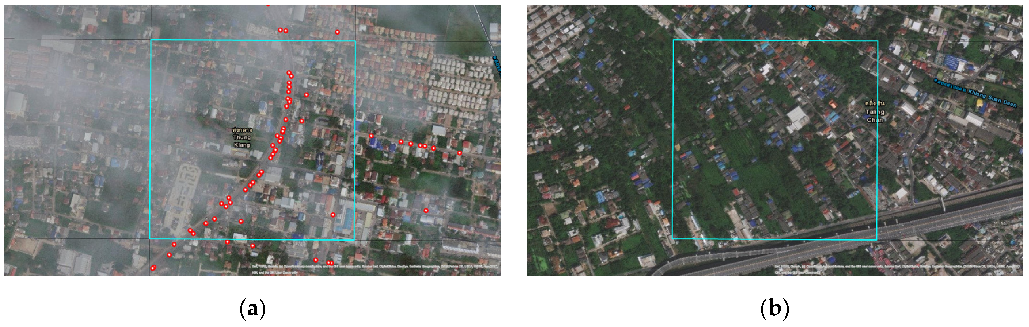
Figure 2 shows the grid area with the location of road traffic injury incidents in the high and low road traffic injury grid, respectively. The number of red dots represents the frequency of road traffic injuries.

2.2.3. Road Traffic Injury Risk Prone Areas

To analyze the relationship between factors related to road traffic injuries, the researchers were required to create a road traffic injury risk prone area map to store the data of dependent variables on the map. All independent variables were then added to the map. Finally, we took a statistical analysis to find the independent variables related to the dependent variables. For the preparation of the road traffic injury risk prone area map, the researchers used kernel density estimation techniques to manage the data-dependent variables.

The kernel density estimation (KDE) method has been considered as one of the best approaches to study and explain the spatial patterns that exist in various parameters [22]. Compared to methods such as the statistical hotspot and clustering approaches, KDE has been found to produce better results. KDE is more advantageous as the use of the density function allows one to define an arbitrary spatial unit that is homogenous for the given area. This ultimately assists in the comparison and classification task.

A count model was used to aggregate the preprocessed data. Furthermore, KDE was used to generate a probability distribution function for the POI features. The natural breaking algorithm was applied to identify the optimal arrangement of POI density values, and the clusters were then reclassified.

In KDE, an asymmetrical surface is placed over each point, and a mathematical operator is used to evaluate the distance between a reference location and the points. The distances from the reference location to all the points on the surface.

The density estimates from KDE were classified into several classes based on the levels of the density areas using a natural break cluster. The natural break algorithm was used as it minimizes the inter-class variance and maximizes the intra-class variance. This algorithm iteratively calculates the breaking points to obtain the sets of breaks with minimum in-class variation and maximum between-class variation. The ordered data were divided into groups.

The independent variables of this study are environmental factors, such as point of interested road and the NDBI, and the dependent factor of this study is the road traffic injury risk prone area.

The classes of accident severity, which are the numbers of traffic accidents with injuries per grid unit (50 m × 50 m) per period, were examined in the grid. The study’s period for training was the calendar year of 2017 and that for testing was the calendar in 2018. The sequence was divided into the following three levels:

• A low number of injured persons per a grid had an accident severity of 0–2 cases.
• A moderate number of injured persons per a grid had an accident severity of 2–15 cases.
• A high number of injured persons per a grid had an accident severity of more than 15 cases.

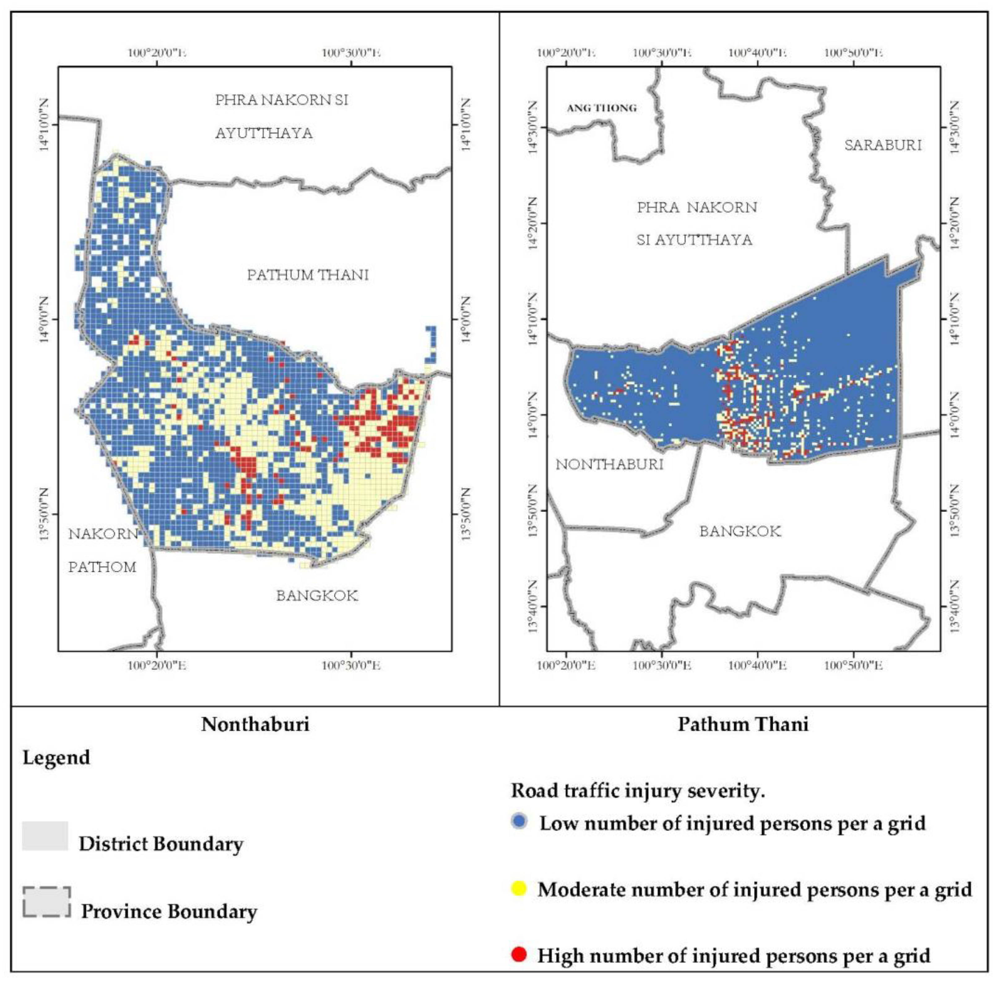
Figure 3 shows the road traffic injuries and risk-prone area severity distribution in Nonthaburi and Pathum Thani Provinces. The database used for road traffic injury severity analysis also includes other independent variables for each crash: point of interest, road characteristics, and urban index, as shown in

Table 4. Characteristic parameters of the road environment in Nonthaburi Province in 2017.

	Mean			Standard Deviation
	Low Number of Injured Persons	Moderate Number of Injured Persons	High Number of Injured Persons	Low Number of Injured Persons	Moderate Number of Injured Persons	High Number of Injured Persons
Grocery	0.14	0.29	0.47	0.50	0.70	1.12
Convenience	0.07	0.38	0.73	0.33	0.93	1.34
Home goods	0.14	0.29	0.47	0.50	0.70	1.12
Clothing	0.04	0.15	0.20	0.22	0.51	0.83
Electronic	0.05	0.16	0.36	0.26	0.48	0.71
Furniture	0.05	0.17	0.37	0.28	0.59	0.96
Car repair	0.04	0.16	0.27	0.22	0.53	0.58
Hardware	0.01	0.02	0.02	0.11	0.16	0.13
Health	0.01	0.04	0.07	0.10	0.24	0.25
Pet	0.01	0.05	0.03	0.12	0.26	0.18
Bicycle	0.01	0.03	0.03	0.09	0.20	0.18
Drugstore	0.01	0.02	0.05	0.11	0.15	0.22
Supermarket	0.01	0.01	0.03	0.09	0.11	0.18
Shoe	0.00	0.03	0.05	0.07	0.29	0.29
School	0.05	0.23	0.24	0.26	0.56	0.60
Gas station	0.08	0.43	0.66	0.41	1.06	1.31
Food store	0.76	2.87	4.46	2.25	4.77	5.85
Length	1.35	1.69	1.81	0.48	0.46	0.39
Intersection	2.50	2.70	2.73	0.54	0.58	0.52
NDBI	2.49	2.64	2.69	0.56	0.57	0.50

and

Table 5. Characteristic of road environment in Pathum Thani Province in 2017.

	Mean			Standard Deviation
	Low Number of Injured Persons	Moderate Number of Injured Persons	High Number of Injured Persons	Low Number of Injured Persons	Moderate Number of Injured Persons	High Number of Injured Persons
Grocery	0.11	0.60	1.25	0.49	1.17	1.43
Convenience	0.04	0.63	1.29	0.30	1.04	1.63
Home goods	0.04	0.29	0.61	0.24	0.63	0.99
Clothing	0.01	0.14	0.25	0.13	0.54	0.59
Electronic	0.03	0.31	0.46	0.30	0.84	1.10
Furniture	0.03	0.36	0.64	0.23	0.96	1.25
Car repair	0.03	0.28	0.75	0.37	1.41	1.11
Hardware	0.01	0.07	0.04	0.11	0.26	0.19
Health	0.01	0.02	0.07	0.09	0.13	0.26
Pet	0.00	0.04	0.11	0.08	0.18	0.31
Bicycle	0.00	0.06	0.07	0.06	0.27	0.26
Drugstore	0.00	0.05	0.07	0.08	0.23	0.26
Supermarket	0.01	0.01	-	0.08	0.10	-
Shoe	0.00	0.04	-	0.06	0.18	-
School	0.04	0.24	0.36	0.24	0.60	0.87
Gas station	0.05	0.50	1.18	0.33	1.06	1.81
Food store	3.45	7.25	1.43	5.15	7.02	3.45
Length	1.41	1.81	2.00	0.50	0.42	-
Intersection	2.51	2.69	2.68	0.57	0.50	0.55
NDBI	2.51	2.62	2.61	0.58	0.52	0.50

.

Road traffic injury risk prone area severity was classified into three levels. level 1, representing low-frequency injuries, which accounted for 59.8% of the total crashes in Nonthaburi Province and 87.54% of the total crashes in Pathum Thani Province; level 2, denoting moderate-frequency injuries, which accounted for 33.95% of the total crashes in Nonthaburi Province and 9.24% of those in Pathum Thani Province; and level 3, representing high-frequency injuries with small proportions of 6.25% and 3.22% of the total crashes in Nonthaburi and Pathum Thani, respectively. The road traffic injury risk prone area severity distribution in Nonthaburi and Pathum Thani is shown in Figure 3.

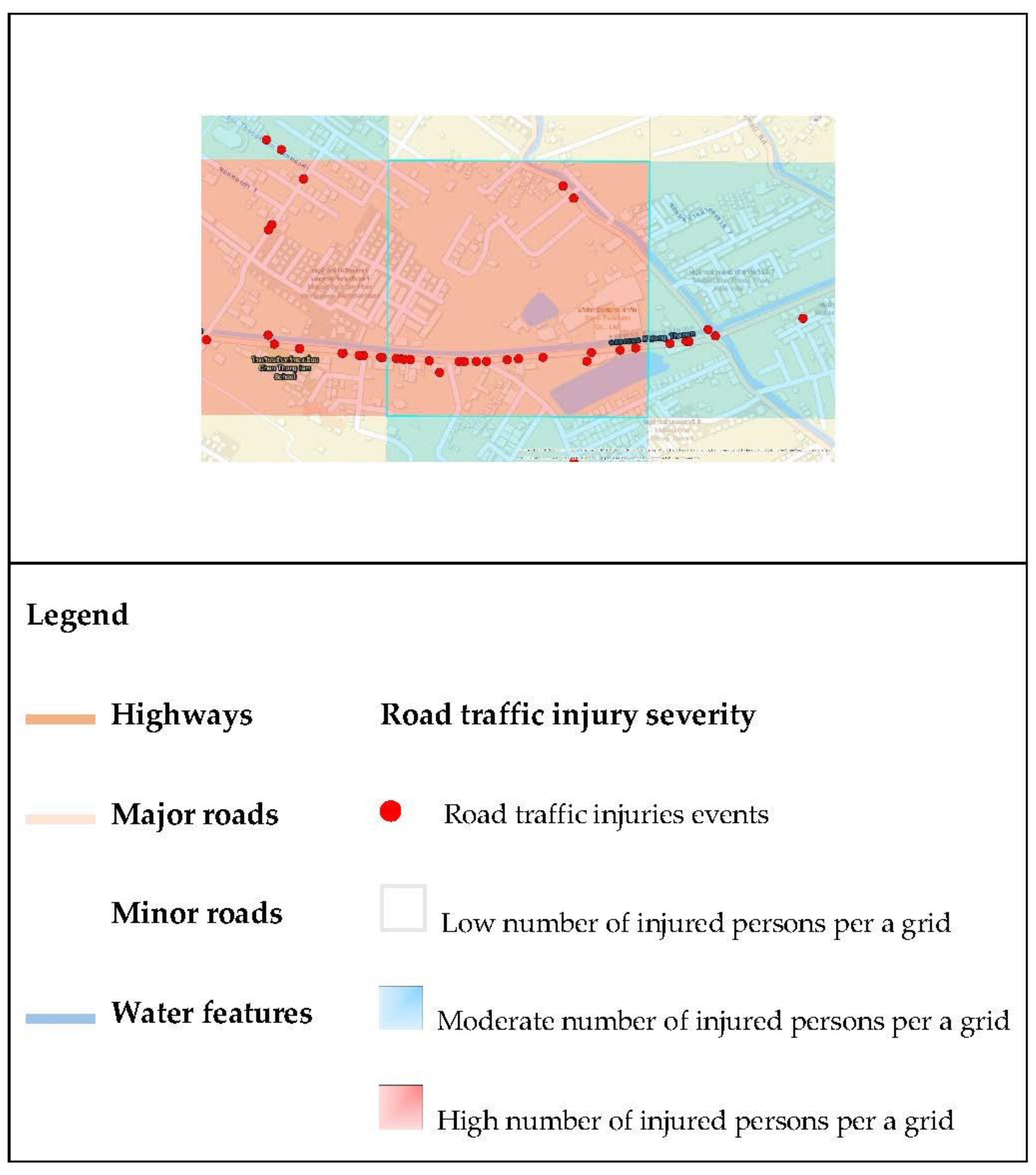
Figure 4 shows examples of environmental factors, such as roads of various sizes, water features, and land use. The transparent red box represents the high-frequency injury area. The transparent blue box represents the moderate-frequency injury area, and the remaining area represents the low-frequency road traffic injury area.

Table 4 and Table 5 shows each data layer’s average and standard deviation by splitting the data into three groups: first, a low number of injured persons per grid; second, a moderate number of injured persons per grid; and third, a high number of injured persons per grid.

The class of independent variables analyzed from the grid is the number of independent variables with a grid unit (50 m × 50 m) per period. The grid was regrouped by using kernel density estimation values from road traffic injuries previously mentioned in the Section 2.2.3; the independent variables obtained from each group of road traffic injuries were counted, and the descriptive statistic of each groups are shown.

Table 4 and Table 5 show the low number of injuries in the grid in Nonthaburi; the most common POIs in Nonthaburi’s grid are restaurants, which is the same for Pathum Thani. Restaurants displayed the same value in both the moderate and low numbers of injured persons sections. In the high number of injured persons sections, restaurants, and gas station can be observed. It is noted that as the number of injuries increases, the average of each type of data increases accordingly.

The relationship between the dependent variable and the independent variable can be summarized with the following mathematic equation:

$${\mathrm{Y} = \mathsf{\beta }}_0{ + \mathsf{\beta }}_1{\mathrm{X}}_1{ + \mathsf{\beta }}_2{\mathrm{X}}_2{ + \dots + \mathsf{\beta }}_{\mathrm{i}}{\mathrm{X}}_{\mathrm{i}}$$

$$\mathrm{Y} = \mathrm{Dependent} \mathrm{variable} \mathrm{or} \mathrm{road} \mathrm{traffic} \mathrm{injuries};$$

$${\mathsf{\beta }}_0= \mathrm{Intercept};$$

$${\mathsf{\beta }}_{\mathrm{i}}{ = \mathrm{Slope} \mathrm{for} \mathrm{X}}_{\mathrm{i}};$$

$$\mathrm{X} = \mathrm{Independent} \mathrm{variable} \mathrm{or} \mathrm{environmental} \mathrm{variables}.$$

2.3. Overall Methodology

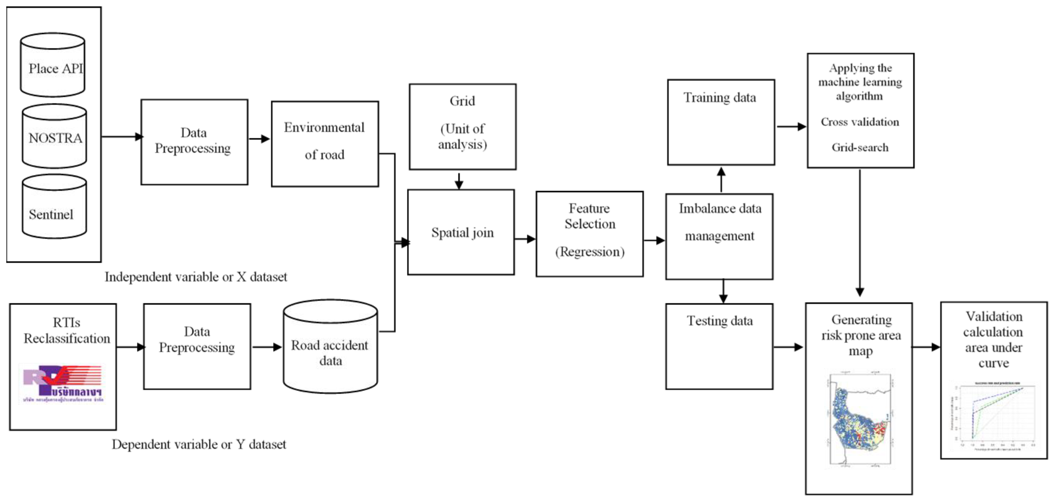
Figure 5 shows the flow chart of machine learning algorithms for the classification of road traffic injury risk prone areas.

To analyze the correlation between environmental factors and road traffic injury risk prone areas, the relevant factors were collected from Place API, the road, and Sentinel maps. Each unit analysis in the training dataset has a label that indicates the road traffic injury risk prone area level (dependent variable), as they are paired with individual environmental factors (independent variables).

A multiple linear regression model was developed to analyze the relations between the response (dependent) variable and the predictor (independent) variables. The annual frequency of road traffic accidents was used as the basic variable to conduct statistics and analysis. Regression analysis helps in understanding the association between one or more predictor (independent) variable and one continuous dependent (or outcome) variable. In regression analysis, the dependent and independent variables are denoted by “Y” and “X”, respectively. Thus, in this research, “Y” represents the road traffic injuries and “X” represents environmental variables.

From the research methodology, an important challenge is class imbalance data management. Imbalanced classification issues are common in many science fields, To overcome imbalanced dataset problem, many approaches have been developed. As the road safety domain is based on a matched case–control design [23], synthetic minority oversampling [24,25], or a combination of minority over-sampling and maximum dissimilarity undersampling [26], the production of a balanced training dataset was proposed in this study. The algorithm area is based on bootstrap aggregation [27].

The synthetic minority oversampling technique (SMOTE) is a popular oversampling technique that generates new synthetic datasets around the minority samples. The synthetic data for the minority classes are generated by interpolating around the nearest neighbors of the consecutive minority class [28]. The SMOTE is useful for well-sampled lower dimensional data compared to higher dimensional data. The generative bias (the generation of synthetic instances within majority classes or not near the minority classes) in the good samples’ lower dimension data is lower. The combination of bootstrap aggregation (bagging) and under-sampling has been found to outperform other strategies for handling imbalanced datasets [29].

In this research, balanced bootstrap training samples were generated, and then an ensemble of classifiers were used for classification task [29].

The strategy implemented is as follows:

• Random splitting of the dataset into training and test datasets in the ratio of 70:30.
• From the training set, n bootstrap samples are taken.
• Random down sampling is used to balance each of the samples.
• A classifier is trained to the balanced samples.
• The classifier is used on the test dataset, and the outcome is predicted.
• The final decision is made based on majority voting.
• The metrics are derived using the model’s outcomes and the actual observation in the holdout, and the classifier’s performance is assessed.

The process is iterated n times to obtain robust results; thus, it is somewhat similar with a nested cross-validation concept [30]. In the present case, n = 5 iterations (i.e., ensembles) features different randomly sampled training and test datasets as they are carried out.

Machine learning algorithms were then implemented using a grid search. Grid search is the process of scanning the data to configure optimal parameters for a given model. The grid search approach can be implemented across a variety of machine learning algorithms to identify the best parameter combination [31].

Once the best model was obtained using the grid search, the model’s performance was assessed on the test data. By comparing the predicted and observed severity of road traffic injury risk prone area levels, the accuracy, which indicates the correctly classified proportion, was calculated. Accuracy indicated the model’s classification performance.

In this study, we used three machine learning algorithms, namely, naïve Bayes, a support vector machine, and random forest. This is because (1) the naïve Bayes classifier is a quick and simple algorithm that can solve various classification problems, and it is easy to implement, as only the probability is calculated. (2) SVM works well when there is a clear margin of separation between classes and excellent theoretical guarantees regarding overfitting. It can work well with an appropriate kernel even if data are not linearly separable in the base feature space, and it is often used for text classification problems that have very high dimensions. (3) Random forest works well with nonlinear data and large datasets. Like SVMs, it seems to be quite popular nowadays, but it has some advantages over SVMs, such as its fast speed and scalability, and it does not concern many parameters like SVM does. All of these algorithms have their own merits.

As previously mentioned, three machine learning algorithms, SVM, naïve Bayes, and random forest, were assessed in this research. In addition, this study also used cross-validation and grid search techniques to reduce the risk of losing important patterns/trends in the dataset, which in turn increases error induced by bias.

In road traffic injury modeling, the primary step was the development of the models, which was conducted over several phases. The data were randomly split into two sets: training and validation sets, and there are three research questions of this study. For this study, machine learning was tested in terms of two research questions.

First research question: Can machine learning predict road traffic injuries in the same study area but for different years?

Second research question: Can machine learning of a road traffic injury model for the Nonthaburi area predict road traffic injuries in the Pathum Thani area?

3. Experiments and Results

3.1. Variable Control for the Machine Learning Model

The experiment was divided into three types: own province with a different year, dataset, own province with a different area dataset, and own province for the grid search. The first research question is as follows: can machine learning predict road traffic injuries in the same study area but for different years?

In the first case (different year dataset), the dataset for 2017 was used to train the model, and the dataset for 2018 was used for validation. In Nonthaburi Province, 2639 records in 2017 were used for model development, and 2639 records in 2018 were used to test the model’s performance. Likewise, in Pathum Thani Province, 6302 records from 2017 were used for the development of the model, and 6302 records from 2018 were used for the validation of the model.

The second research question is as follows: can machine learning of the road traffic injuries in the Nonthaburi area predict road traffic injuries in the Pathum Thani area?

In the second case (different area dataset), the dataset of Nonthaburi Province in 2017 was used for model development, and the model was tested in Pathum Thani Province for the same year. Thus, 2639 records from Nonthaburi Province were used for the development of the model, and 6302 records from Pathum Thani were used to validate the developed model for implementation in Pathum Thani Province.

3.2. Validation Methods

An assessment of the model’s performance using an imbalanced dataset may not be reliable, as the performance metrics used to evaluate the quality of the model may result in misleading conclusions.

Several metrics can be calculated and used to describe and evaluate the quality and overall predicted performance of the machine learning models. For the classification task, most of the metrics can be derived from the confusion matrix. The confusion matrix is a two-dimensional contingency matrix that illustrates the performance of classifiers on a set of test data whose actual values are already known.

ACC = “TP+TN”/“TP + FN + FP + TN”

SST = “TP”/“TP + FN”

SPE = “TN”/“TN + FP”

PPV = “TP”/“TP + FP”

NPV = “TN”/“TN + FN”

F1 = 2 × “PPV × NPV”/“PPV + NPV”

where TP represents true positive, TN represents true negative, FP represents false positive, FN represents false negative, TC represents the correctly classified pixel count, and TD represents the incorrectly classified pixel count. A represents the road traffic injury pixel count, B represents the non-road traffic injury pixel count, N represents the number of samples in the dataset, ${\mathrm{y}}_i$ represents the predicted value of the ith sample, and ${\overline{\mathrm{y}}}_i$ represents the measured value of the ith sample.

Accuracy (ACC) indicates the ability of a binary classification test to identify or exclude an outcome correctly. It is the ratio of correct predictions to the total number of samples. When the dataset is severely imbalanced, the overall accuracy is not enough to explain the performance of the model, as the overall accuracy can be higher with most of the samples being classified into majority class.

Sensitivity (SST), or exact positive rate or recall, is the ratio of correctly classified positives to the total number of samples that are actually positives. As sensitivity represents the correct classification rate of the accident class, it is an important indicator to evaluate and compare classifiers with.

Specificity (SPE), or exact negative rate, is the ratio of correctly classified negatives to the total number of samples that are actually negative. Specificity is nearly identical to accuracy as the number of events are lower.

Precision, or positive predictive value (PPV), is the ratio of correctly classified positives to the total number of samples that are classified as positives.

Fallout, also known as the false-positive rate (NPV), is the ratio of correctly classified negatives to the total number of samples that are classified as negatives. It represents the percentage of “false alarms” and is a complementary rate to specificity.

The F1 score is computed as the harmonic mean of precision and sensitivity.

3.3. Training of Naïve Bayes, Random Forest and Support Vector Machine, and Generation of the Road Traffic Injury Risk Prone Area

3.3.1. Support Vector Machine

In the case of SVM, this model with its optimal parameters for searching played a crucial role in the performance of the model. The kernel function used in this research was the radial basis function (RBF). The training process was initiated by using a grid search approach to search for the optimal kernel parameters. To prevent overfitting, five-fold cross-validation was implemented with the grid search. Thus, the training dataset was randomly divided into five equally sized subsets. Each subset was used as a test dataset for the SVM model developed from the remaining four chunks. The cross-validation process was then repeated five times with each of the five subsets used once as a test dataset.

The two kernel parameter influencing the RBF kernel function are $\complement$ and γ. The following procedure was used: (1) a grid space of ($\complement$, γ), where $\complement$ = $2^{-5}$, $2^{-4}$, …, $2^{10}$ and γ = $2^{10}$, $2^9$, …, $2^{-4}$, was set; (2) for each parameter, using the pair of ($\complement$, γ) in the grid space, five-fold cross-validation on the training dataset was conducted; (3) the parameter pair of ($\complement$, γ) that had the highest accuracy classification was chosen; (4) finally, the best parameters were used to construct an SVM model for road traffic injury predictions. The best $\complement$ and γ were determined as 128 and 0.11342, respectively. The correctly classified rate of 91% was obtained. The Support vector machine with the radial basis function (RBF) kernel grid search results was shown in

Table 6. Support vector machine with the radial basis function (RBF) kernel grid search results.

Sigma	C	Accuracy	Kappa
0.11	0.25	0.83	0.74
0.11	0.50	0.85	0.78
0.11	1.00	0.87	0.81
0.11	2.00	0.88	0.82
0.11	4.00	0.89	0.84
0.11	8.00	0.90	0.85
0.11	16.00	0.90	0.85
0.11	32.00	0.90	0.86
0.11	64.00	0.90	0.86
0.11	128.00	0.91	0.86

Tuning parameter “sigma” was held constant at a value of 0.11. The final values used for the model were sigma = 0.11 and C = 128.

.

3.3.2. Random Forest

Random forest includes an implementation of probability forests for estimating individual probabilities for response, according to Malley et al. (2012), where the forest probability estimate is obtained as the average of all probability estimates for every single tree. A detailed accuracy assessment for Random Forest is shown in

Table 7. Random Forest grid search results.

mtry	Accuracy	Kappa
1.00	0.75	0.62
2.00	0.86	0.78
3.00	0.91	0.86
4.00	0.91	0.87
5.00	0.91	0.87
6.00	0.92	0.87
7.00	0.92	0.87
8.00	0.92	0.87
9.00	0.92	0.87
10.00	0.92	0.87
11.00	0.92	0.87
12.00	0.92	0.88
13.00	0.92	0.88
14.00	0.92	0.88
15.00	0.92	0.88

The final value used for the model was mtry = 13.

. It can be observed that the precision, F-measure, and TP rates are all higher (>90%) than the FP rate (<10%). This implies that the model shows good performance for the training dataset, and there is good agreement between the observed and the predicted values. The best mtry was 13. The correctly classified rate of 92% was obtained.

3.3.3. Naïve Bayes

Naïve Bayes computes the probability of each output class, and then the classification is performed for the class with the higher posterior probability. The NB model obtained an overall classification accuracy of 82.6%.

Table 8. Naïve Bayes grid search results.

	Usekernel	fL	Adjust	Accuracy
1	TRUE	1	5	0.826
2	TRUE	0	5	0.825
3	TRUE	2	5	0.824
4	TRUE	3	5	0.823
5	TRUE	4	5	0.822

The final values used for the model were fL = 1, usekernel = TRUE and adjust = 5.

shows the model assessment and performance results.

After the models (SVM, RF, and NB) were trained and the outputs were generated, open-source geospatial software (QGIS) was used for further analysis.

3.4. Results

3.4.1. Factor Importance

Table 9. Variable ranks extracted using the regression selection method.

Estimate	Std.	Error	t Value	Pr (>|t|)	Std.
(Intercept)	30.4472	6.8302	4.458	0.00000857	***
Grocery	16.879	0.5018	33.635	<2 × 10−16	***
Convenience	10.2248	0.8601	11.888	<2 × 10−16	***
Electronics	−10.1203	0.7483	−13.524	<2 × 10−16	***
Drugstore	−31.1778	1.9051	−16.365	<2 × 10−16	***
Restaurant	3.2839	0.9755	3.366	0.00077	***
Length	1.6609	0.4675	3.553	0.000387	***
Supermarket	15.0796	4.1839	3.604	0.000318	***
School	−4.2553	0.637	−6.68	2.81 × 10−11	***
Gas station	5.0706	0.6387	7.938	2.8 × 10−15	***

Signif. codes: 0 ‘***’ 0.001 ‘**’ 0.01 ‘*’ 0.05 ‘.’ 0.1 ‘ ’ 1. Residual standard error: 9.654 on 3214 degrees of freedom. Multiple R-squared: 0.8038, Adjusted R-squared: 0.8027. F-statistic: 731.6 on 20 and 3214 Degrees of Freedom, p-value: <2.2 × 10⁻¹⁶.

shows the results of the multiple linear regression model results and the variable assignments based on quartiles. The regression model showed a relatively high coefficient of determination (R² = 0.80, F = 1511709.75, P < 0.001). It was observed that the regression model fits the data well. Overall important variable metrics are shown in

Table 10. Model development in different years in the Nonthaburi dataset.

Model		Sensitivity	Specificity	Precision	Recall	F1	Accuracy
NB	Low-frequency injury	1.00	0.79	0.68	1.00	0.81	0.89
	Moderate-frequency injury	0.38	0.89	0.65	0.38	0.48	0.64
	High-frequency injury	0.68	0.83	0.69	0.68	0.68	0.76
RF	Low-frequency injury	0.93	0.93	0.85	0.93	0.89	0.93
	Moderate-frequency injury	0.79	0.88	0.77	0.79	0.78	0.84
	High-frequency injury	0.83	0.96	0.92	0.83	0.87	0.89
SVM	Low-frequency injury	0.61	0.91	0.76	0.61	0.67	0.76
	Moderate-frequency injury	0.51	0.72	0.49	0.51	0.50	0.62
	High-frequency injury	0.82	0.83	0.71	0.82	0.76	0.82

. Unsurprisingly, grocery and convenience stores prevailed as the most important features in the regression selection method. In addition, electronics and drug stores were also very important variables in this context.

The results show that certain public welfare factors, including schools and gas stations, are variables of high importance. In addition, two variables related to food, such as restaurants and supermarkets, were related with the highest occurrence rates of road traffic injuries. Road geometrics such as length were statistically significant.

3.4.2. Model Performance

The validations of nine road traffic injury susceptibility maps were performed by comparing them with the level of road traffic injury risk prone area locations using prediction rate methods. The road traffic injury susceptibility map consists of three algorithms in different years in Nonthaburi Province and three algorithms in different years in Pathum Thani Province. Moreover, three algorithms using the Nonthaburi 2018 dataset for training and the Pathum Thani 2018 dataset for testing were used.

This shows that all the models have an excellent prediction capability. The highest prediction capability is from RF, followed by NB and SVM-RBF, respectively.

First research question: can machine learning predict road traffic injuries in the same study area but for different years?

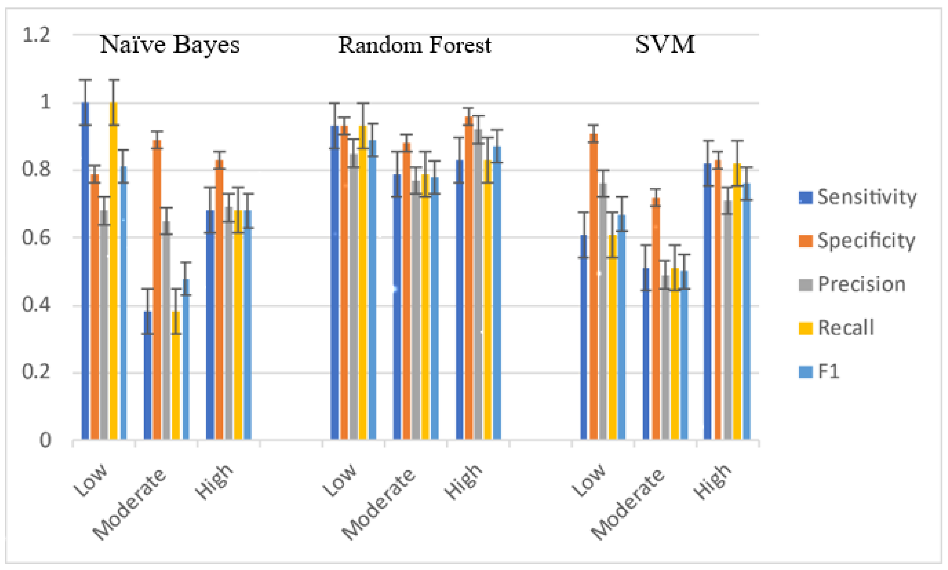
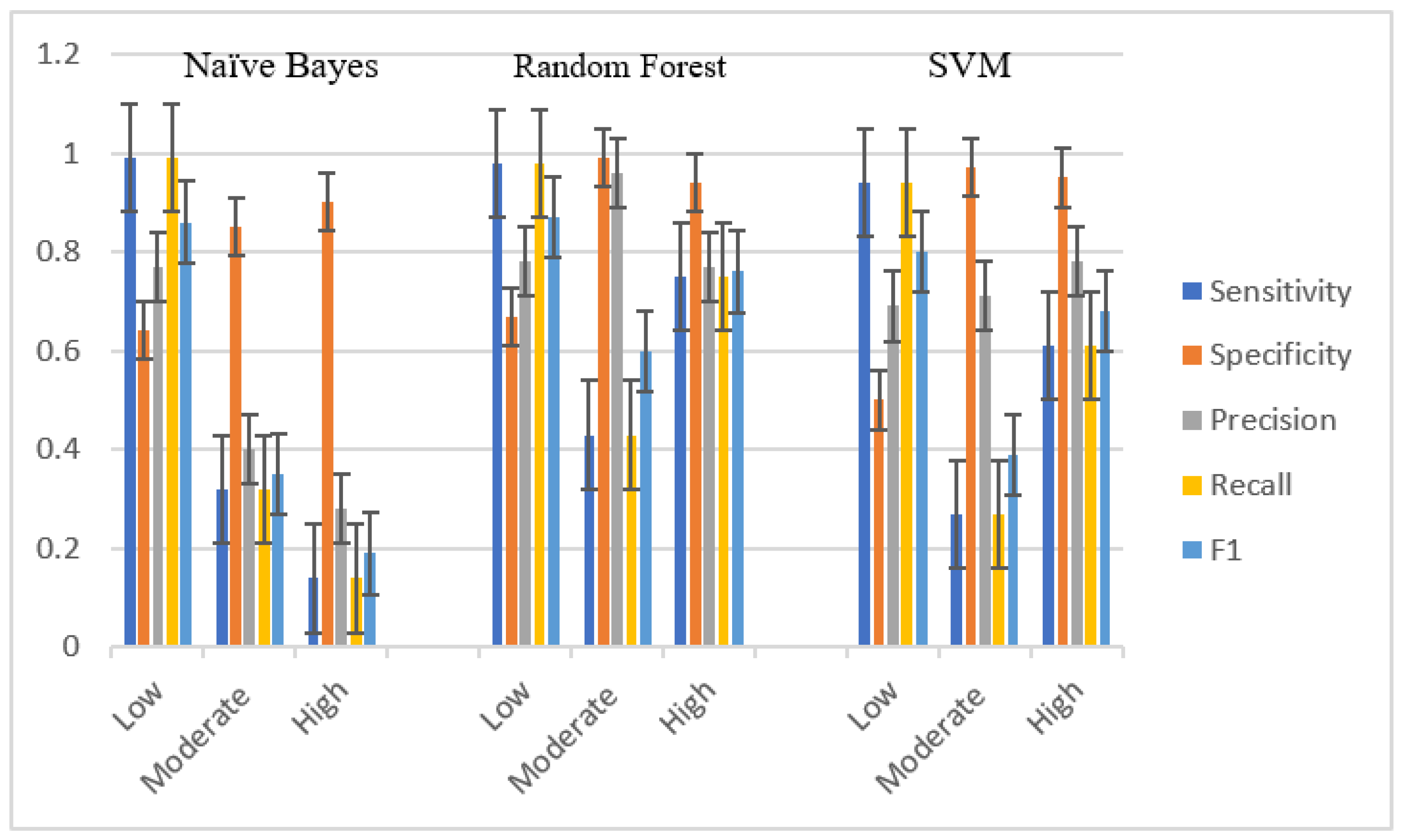
Table 10 and Figure 6 shows the model development in different years in the Nonthaburi dataset. For low-frequency injury cases, NB (1.0) had the highest sensitivity, followed by RF (0.93) and SVM (0.61), respectively. Meanwhile, for moderate-frequency cases, RF (0.79) had the highest sensitivity. RF (0.83) was the same in high-frequency cases. In terms of specificity, it was found that low-frequency RF (0.93) cases had the highest specificity, just as in the high-frequency cases (0.96). Meanwhile, for moderate-frequency cases, NB (0.89) and RF (0.88) gave similar results. When bringing precision and recall to the F1 score to identify the best harmonic mean models, RF had the best F1 score.

Table 11. Model development in different years in the Pathum Thani dataset.

Model		Sensitivity	Specificity	Precision	Recall	F1	Accuracy
NB	Low-frequency injury	1.00	0.82	0.71	1.00	0.83	0.91
	Moderate-frequency injury	0.56	0.85	0.67	0.56	0.61	0.71
	High-frequency injury	0.64	0.91	0.80	0.64	0.71	0.78
RF	Low-frequency injury	0.94	0.89	0.78	0.94	0.85	0.91
	Moderate-frequency injury	0.63	0.86	0.71	0.63	0.67	0.75
	High-frequency injury	0.80	0.92	0.85	0.80	0.82	0.86
SVM	Low-frequency injury	0.88	0.81	0.68	0.88	0.77	0.85
	Moderate-frequency injury	0.72	0.80	0.65	0.72	0.68	0.76
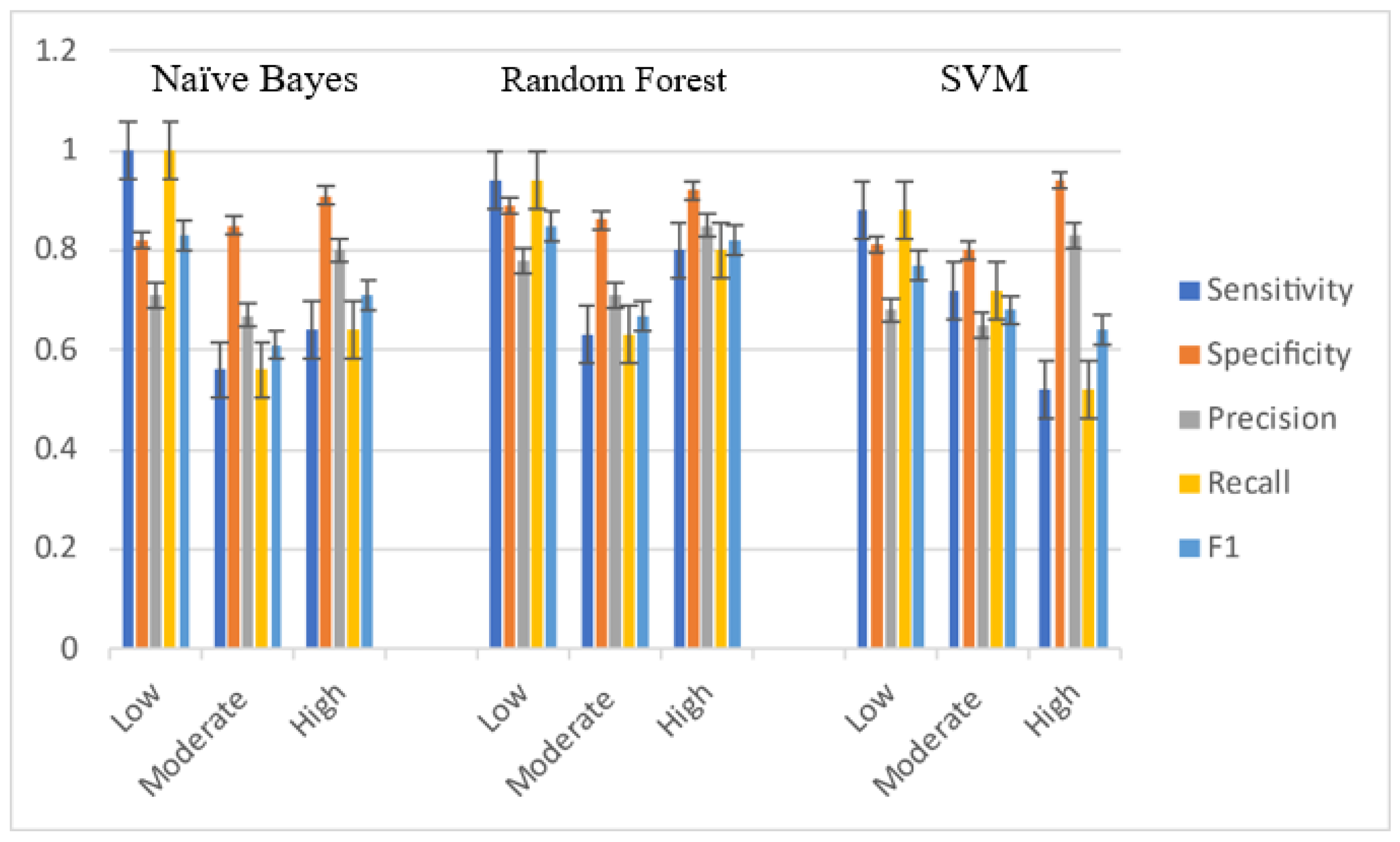
	High-frequency injury	0.52	0.94	0.83	0.52	0.64	0.73

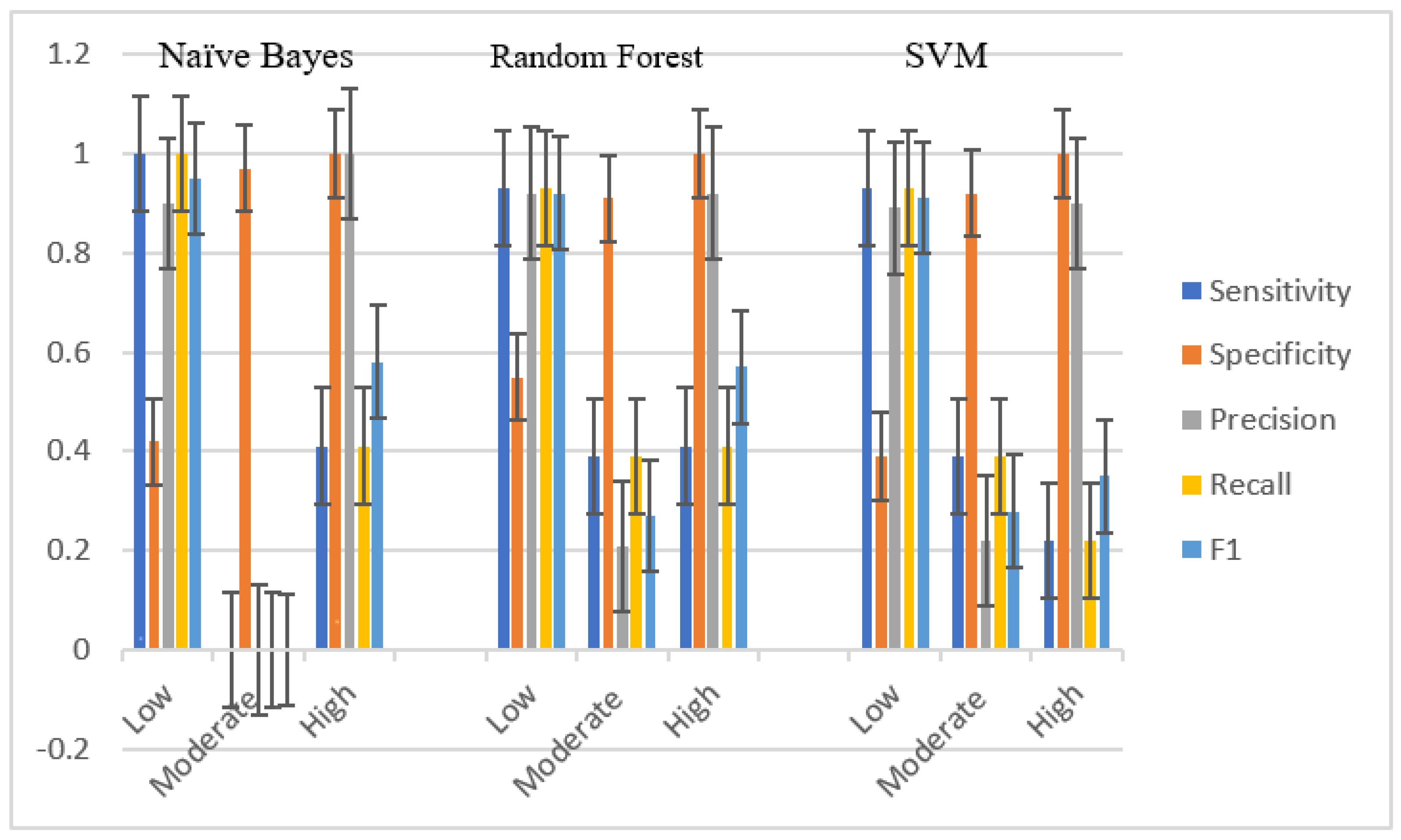
and Figure 7 show model development in different years in the Pathum Thani dataset. For low-frequency injury cases, NB (1) had the highest sensitivity, followed by RF (0.94) and SVM (0.88), respectively. Meanwhile, for moderate-frequency cases, SVM (0.72) had the highest sensitivity, and in high-frequency cases, RF (0.8) had strong sensitivity. In terms of specificity, it was found that in low-frequency cases, RF (0.89) had the highest specificity, and the same was true for moderate-frequency (0.86), while in serious cases, SVM (0.94) was slightly different from RF (0.92) and NB (0.91). When bringing precision and recall to the F1 score to identify the best harmonic mean models, RF had the best F1 score, the same as in Nonthaburi Province.

Second research question: can a machine learning of road traffic injury model for the Nonthaburi area predict road traffic injuries in the Pathum Thani area?

Table 12. Model development for all districts in the Nonthaburi dataset and Pathum Thani dataset.

Model		Sensitivity	Specificity	Precision	Recall	F1	Accuracy
NB	Low-frequency injury	1.00	0.74	0.61	1.00	0.76	0.87
	Moderate-frequency injury	0.65	0.83	0.66	0.65	0.66	0.74
	High-frequency injury	0.47	0.97	0.91	0.47	0.62	0.72
RF	Low-frequency injury	0.77	0.96	0.88	0.77	0.82	0.86
	Moderate-frequency injury	0.79	0.73	0.61	0.79	0.69	0.76
	High-frequency injury	0.69	0.93	0.85	0.69	0.76	0.81
SVM	Low-frequency injury	0.81	0.43	0.36	0.81	0.50	0.62
	Moderate-frequency injury	0.29	0.80	0.44	0.29	0.35	0.55
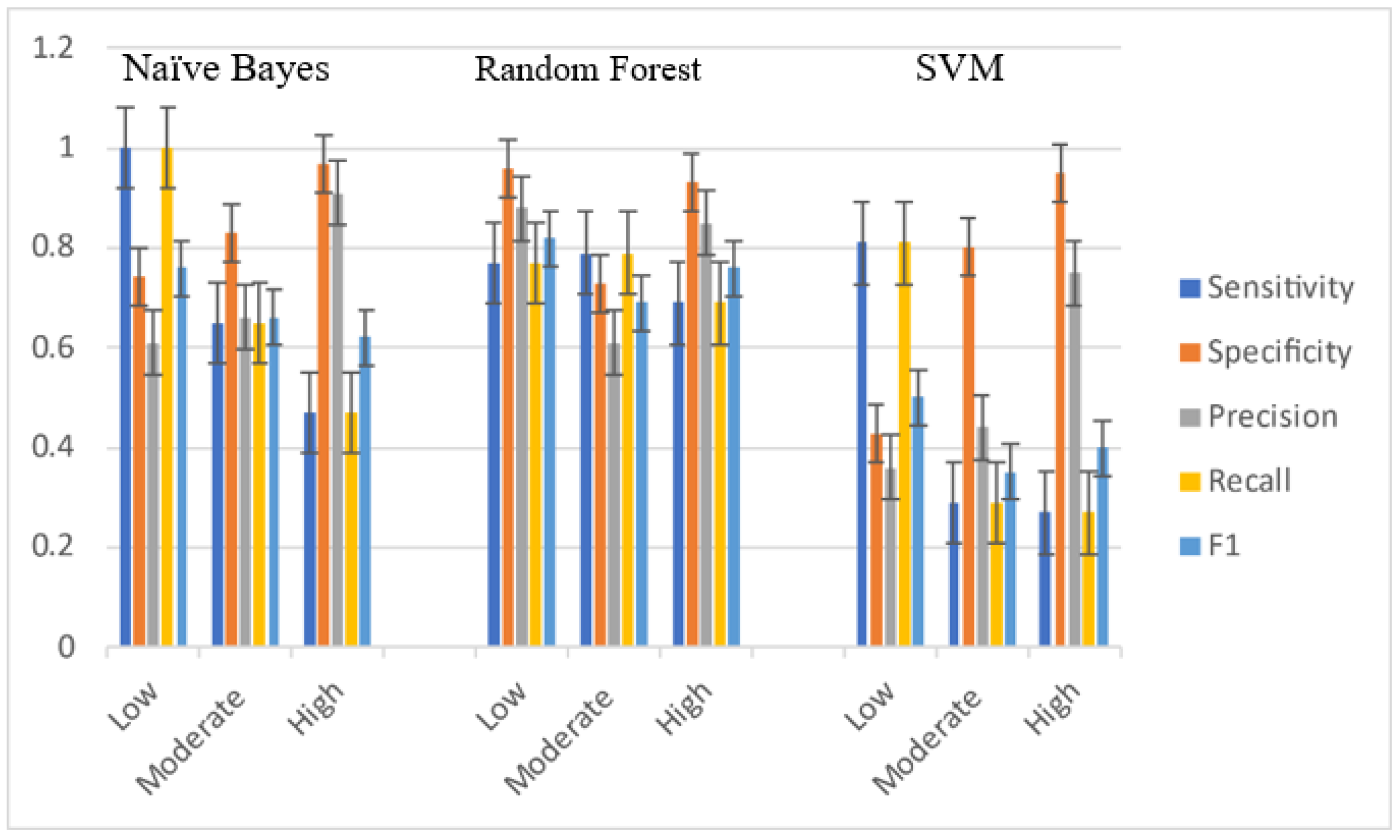
	High-frequency injury	0.27	0.95	0.75	0.27	0.40	0.61

and Figure 8 shows model three in different provinces, the Nonthaburi 2018 training area, and Pathum Thani Province in 2018 as a testing area. It can be observed that RF models have the highest accuracy, the same as that of model one and model two.

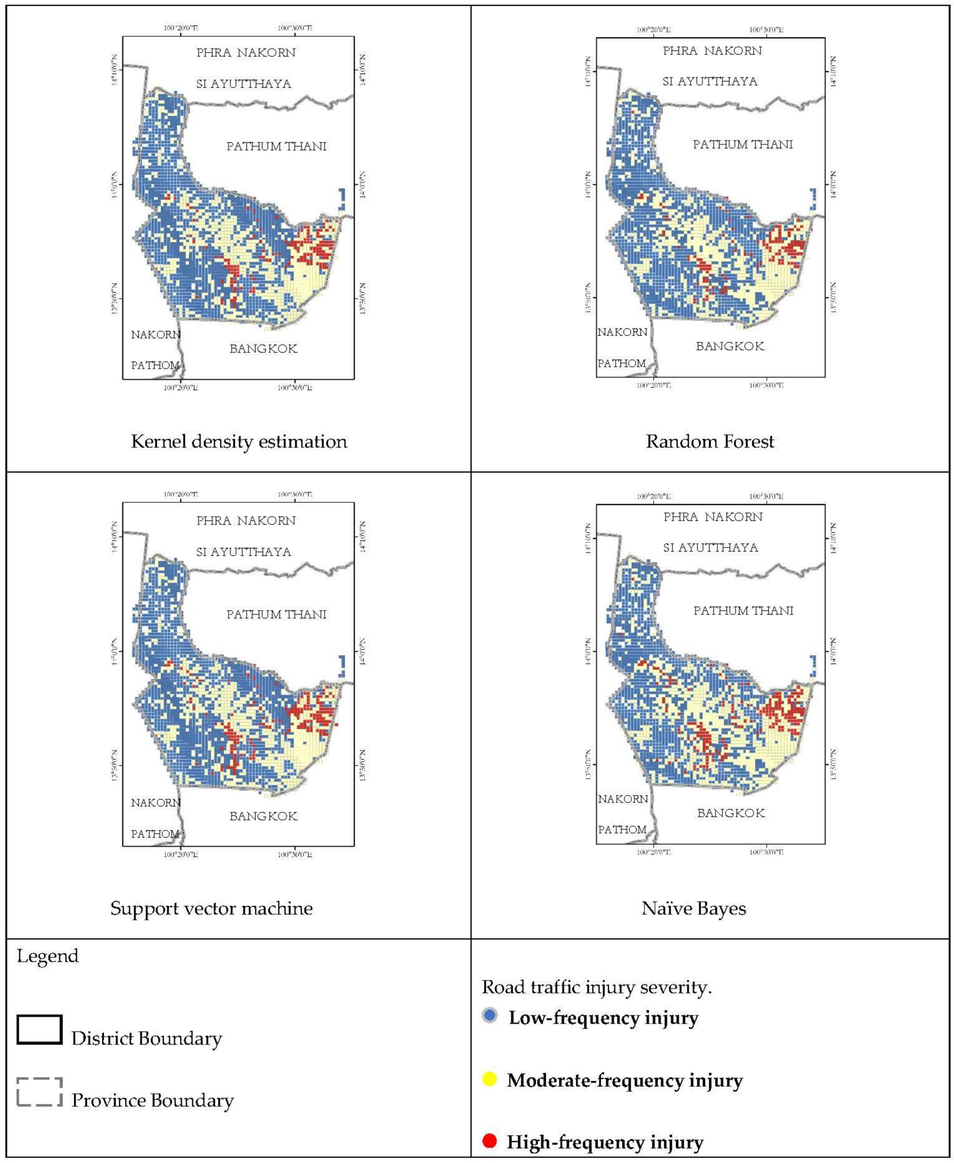
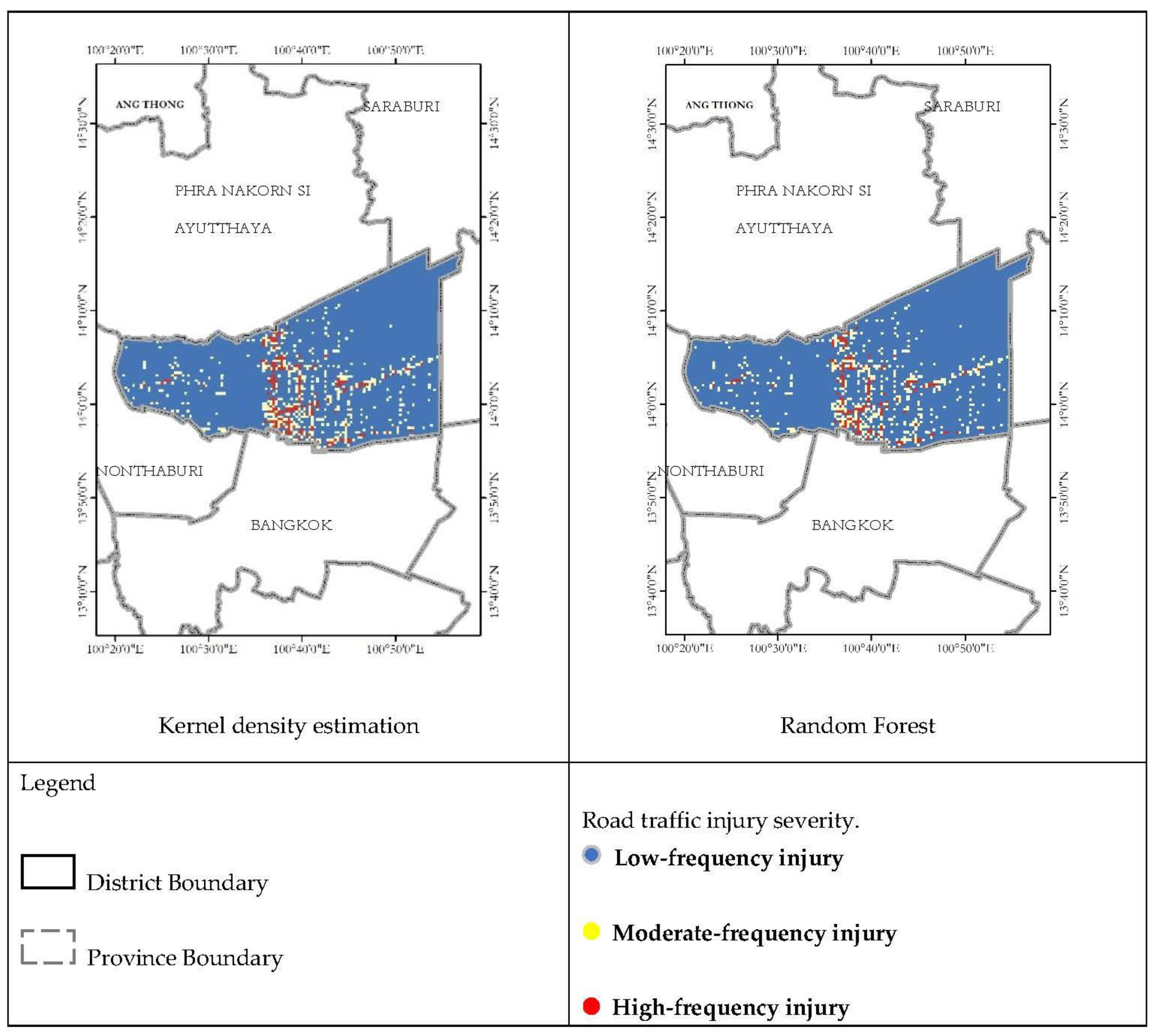
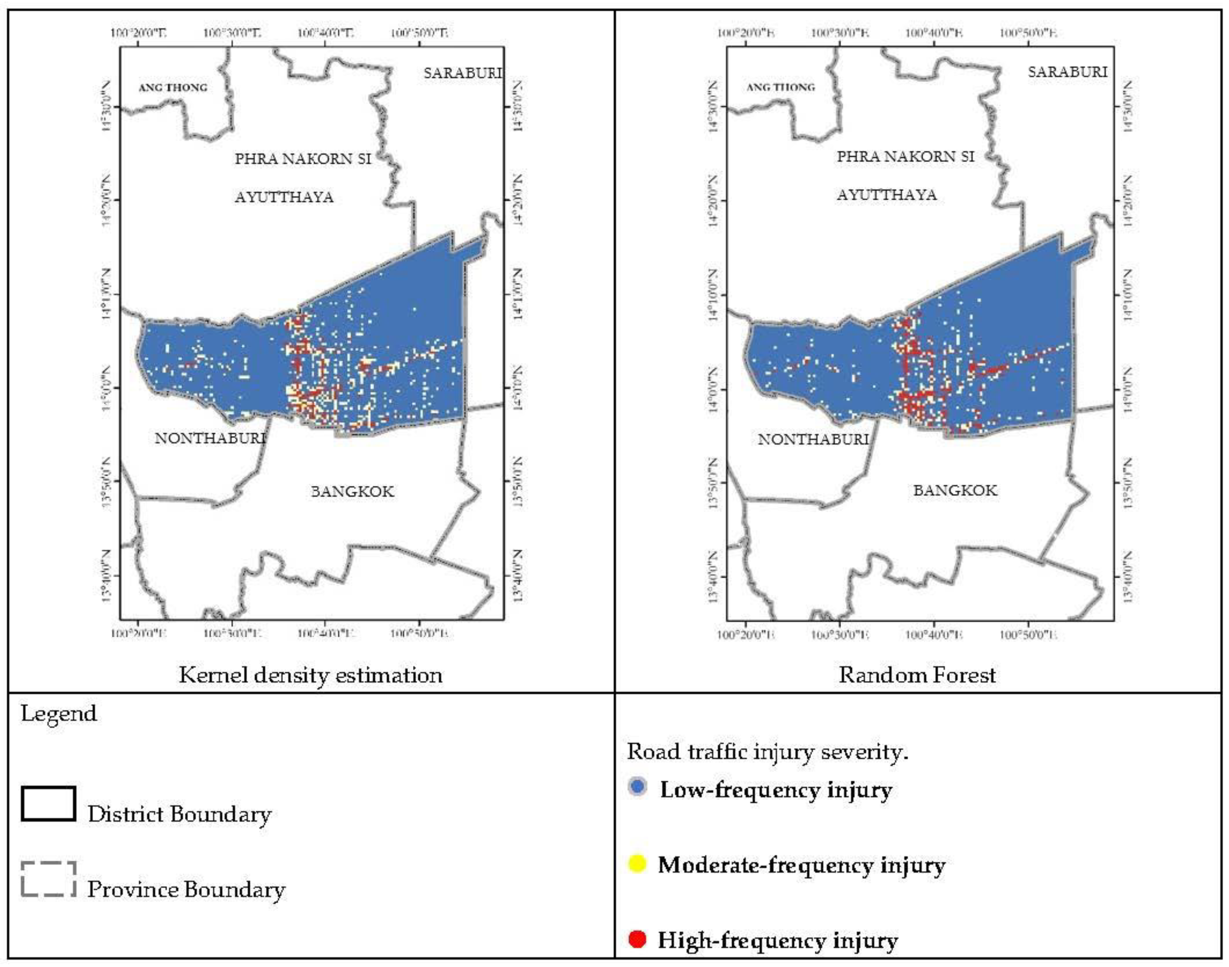
The resulted map of first question was shown in Figure 9 and Figure 10. Then, the resulted map of second research question was shown in Figure 11.

For low-frequency injury cases, NB (1) had the highest sensitivity. Meanwhile, for moderate-frequency cases, RF (0.79) had the highest sensitivity, and in high-frequency cases, RF (0.69) had strong sensitivity. In terms of specificity, it was found that in low-frequency cases, RF (0.96) had the highest specificity, while in moderate-frequency, NB displayed the highest sensitivity (0.83). In serious cases, NB (0.97) was slightly different from SVM (0.95) and RF (0.95, When bringing precision and recall to the F1 score to i the best harmonic mean models, RF had the best F1 score.

All of the developed models were validated and compared with each other using suitable metrics. Finally, the maps representing the road traffic injury risk prone areas of the study area were prepared and classified into low-frequency injury areas, moderate-frequency injury areas, and high-frequency injury areas.

Using critical factors that affect road traffic injuries, main roads and minor roads were examined. Then, the grid model unit that overlaps the main road in the area before training the model was selected. The same step was taken for minor roads in the area.

Table 13. Model development for major road in the Nonthaburi and Pathum Thani dataset.

Model		Sensitivity	Specificity	Precision	Recall	F1	Accuracy
NB	Low-frequency injury	0.99	0.64	0.77	0.99	0.86	0.81
	Moderate-frequency injury	0.32	0.85	0.40	0.32	0.35	0.58
	High-frequency injury	0.14	0.90	0.28	0.14	0.19	0.52
RF	Low-frequency injury	0.98	0.67	0.78	0.98	0.87	0.83
	Moderate-frequency injury	0.43	0.99	0.96	0.43	0.60	0.71
	High-frequency injury	0.75	0.94	0.77	0.75	0.76	0.85
SVM	Low-frequency injury	0.94	0.50	0.69	0.94	0.80	0.72
	Moderate-frequency injury	0.27	0.97	0.71	0.27	0.39	0.62
	High-frequency injury	0.61	0.95	0.78	0.61	0.68	0.78

and Figure 12 show three models in the major road; the major road in Nonthaburi 2017 was a training area, and the major road in Pathum Thani Province in 2017 was a testing area. It can be observed that the RF models have the highest accuracy. However, while the moderate frequency section was not very well classified, the overall accuracy was close to that shown in Table 12.

Table 14. Model development for minor road in the Nonthaburi and Pathum Thani dataset.

Model		Sensitivity	Specificity	Precision	Recall	F1	Accuracy
NB	Low-frequency injury	1.00	0.42	0.90	1.00	0.95	0.71
	Moderate-frequency injury	0.00	0.97	0.00	0.00	0.00	0.49
	High-frequency injury	0.41	1.00	1.00	0.41	0.58	0.70
RF	Low-frequency injury	0.93	0.55	0.92	0.93	0.92	0.74
	Moderate-frequency injury	0.39	0.91	0.21	0.39	0.27	0.65
	High-frequency injury	0.41	1.00	0.92	0.41	0.57	0.70
SVM	Low-frequency injury	0.93	0.39	0.89	0.93	0.91	0.66
	Moderate-frequency injury	0.39	0.92	0.22	0.39	0.28	0.65
	High-frequency injury	0.22	1.00	0.90	0.22	0.35	0.61

and Figure 13 show minor road cases; the predicted results were not as good as expected. However, RF came first in the classification results. The reason may be that the POI of the area was like that of the major road, but there was not a high volume of road traffic, resulting in few road traffic injuries.

4. Discussion and Conclusions

4.1. Discussion

Ratanavaraha et al. [32] studied the factors affecting accident severity on expressways in Thailand by using accident data for the period of 2007 to 2010. The multiple logistic regression technique was applied by identifying factors and their statistical relationships with the severity of crashes, which were categorized into three groups: property damage only, injury accident, and fatal accident. The results of the study were satisfactory. However, it was found that such studies on expressways are clearly factors, but road traffic injuries often occur in dynamic areas. In addition, there are factors that require urgent attention, a considerable amount of time, and a large budget before the government conducts surveys.

As a result of this problem, the data do not catch up to solve the problem. Place API is an alternative to this study. Moreover, supposing the factors change a lot, traditional statistics may not be suitable for data analysis because they cannot play the role of tuning parameters like machine learning algorithms, which can be flexible in supporting data analysis situations that data change.

Therefore, this study focused on using place APIs for experiments, and we intended to use machine learning in many situations to accommodate the area’s changing conditions.

4.2. Conclusions

4.2.1. Factor Importance

The determination of the areas that are high road traffic injury risk prone areas is one of the essential steps in reducing road traffic injuries in Thailand. This study is more robust than previous studies for three main reasons. First, many scholars have performed analysis by splitting the dataset into training and test datasets only. In this study, five-fold cross-validation was used. More robust results were obtained by averaging the outcomes from different models (ensembles), Second, in this study, the models were trained with a grid search, which yielded the most optimal results based on the training data. Third, a repeated cross-validation procedure was applied as a robust method, which aided in preventing over-optimistic performance results in the research.

Thus, we developed an ensemble modeling approach to improve the performance of the model and achieve the most accurate and reliable estimate of road traffic injuries for a risk-prone area map. In this study, a feature selection method was implemented, and the features were ranked based on importance score. It was revealed that grocery stores, convenience stores, electronics stores, drug stores, schools, gas stations, restaurants, supermarkets, and road geometrics such as length were the most critical factors that influenced the road traffic injury risk prone model, because these variables are important elements in the livelihood of the city. Many people need to buy goods for everyday consumption, making the area crowded with people and traffic. These variables are also frequently accessed, so road traffic injuries can easily occur.

4.2.2. Model Performance

We were able to delineate the environmental factors in terms of road traffic injury risk prone areas, and so we used SVM, random forest, and naïve Bayes techniques. Apart from providing a distribution map of road traffic injury risk prone areas for Nonthaburi and Pathum Thani Provinces, the study shows that machine learning, especially random forest, can predict road traffic injury risk prone areas. Likewise, the research results can aid in the development of monitoring systems for protection against road traffic injuries.

Machine learning analysis differs from hotspot analysis, as a historical dataset of road traffic injuries is not required. Machine learning algorithms can predict road traffic injury risk prone areas from various environmental factors and are particularly convenient for assessing the risk of road traffic injury in areas that do not have a historical record of road traffic injuries.

The significance of this research is its contribution to the literature by (1) identifying factors that influence road traffic injuries; (2) illustrating the effectiveness of machine learning algorithms to identify road traffic injury risk prone areas from environmental factors; and (3) verifying the model with different years and province datasets.

The advantages of this study are as follows: (1) the delineation of the environmental factor in terms of road traffic injury risk prone areas; (2) the strengthening of the prompt decision-making process; (3) the incorporation of different stakeholders for a faster and effective decision-making process, (4) the formulation of and suggestions regarding an organizational framework to minimize road traffic injury; and (5) the development of monitoring systems for protection against and the prevention of road traffic injury.

The limitation of this study is that the dataset is used in a static format. This may result in the need to update the data and the model frequently.

This study is a multidisciplinary approach based on algorithms used for diagnoses in many fields, and a machine learning approach was developed. The developed approach can be used in many fields with suitable modifications. The integration of dynamic data can help to overcome the limitations caused by a continuously transforming city.