Article

Mode Choice Change under Environmental Constraints in the Combined Modal Split and Traffic Assignment Model

Department of Data Centric Problem Solving Research, Korea Institute of Science and Technology Information, Dajeon 34141, Korea
Sustainability 2021, 13(7), 3780; https://doi.org/10.3390/su13073780
Submission received: 26 February 2021 / Revised: 23 March 2021 / Accepted: 24 March 2021 / Published: 29 March 2021
(This article belongs to the Special Issue New Perspectives on Transportation Mode Choice Decisions)

Abstract

:
With the increasing level of air pollution and fine dust, many countries are trying to prevent further environmental damage, with various government legislations, such as the Kyoto Protocol and the Paris Agreement. In the transportation field, a variety of environmental protection schemes are also being considered (e.g., banning old diesel vehicles, alternate no-driving systems, electric car subsidies, and environmental cost charging by tax). Imposing environmental constraints is a good approach to reflect various environmental protections. The objective of this research was to analyze the mode-choice and route-choice changes based on imposing environmental constraints. For the objective, a combined modal split and traffic assignment (CMA) model with an environmental constraint model was developed. For the environmental constraint, carbon monoxide (CO) was adopted, because most of the CO emissions in the air are emitted by motorized vehicles. After a detailed description of the model, the validity and some properties of the model and algorithm are demonstrated with two numerical examples (e.g., a small and a real network in the city of Winnipeg, Canada). From the numerical results, we can observe that imposing the small restriction (or strict) value has more efficiency in mode change and reducing network emission.

1. Introduction

It is well-known that the transportation system increases the level of air pollution. As the number of motorized vehicles increases, the congestion level on a road network is also increased. From the increased congestion level, the level of air pollution is increased. As a result, environmental deterioration is accelerating. Based on the United States Environmental Protection Agency [1,2], 35% of carbon dioxide (CO2) emissions are contributed by transportation, and the greatest sources of carbon monoxide (CO) in outdoor air are motorized vehicles (e.g., passenger car and truck). Kheirbek [3] estimates the emissions contributed by motorized vehicles in New York City. According to their research, motorized vehicles produced 1817 tons of particulate matter (PM2.5), 43,934 tons of nitrogen oxides (NOx), 20,613 tons of total Volatile Organic Compounds (VOCs), and 336 tons of sulfur dioxide (SO2), and these values are 17.5%, 38.3%, 21.9%, and 4.6% of emissions, respectively. Kim [4] analyzed the greenhouse gas emissions emitted from the transportation sector in Korea and showed that the GHG growth rate emitted from the transportation sector is higher than those emitted from other sectors. From the issues, many countries are trying to prevent further environmental damage with various government legislations (i.e., Kyoto Protocol [5] and the Paris Agreement [6]). For the alleviation of the environmental deterioration, transportation authorities have an effort on the implementation of traffic management strategies and traffic-control policies. For example, old diesel vehicles are banned on the road in Korea, German, India [7,8,9], etc., and an alternate no-driving system [10] starts in Korea. However, most environmental protections only focus on alleviating the environmental deterioration, without considering travel behaviors. Hence, more systematic modeling is required for long-term transportation planning.
Imposing environmental constraints is a good approach to reflect various environmental protection [11]. When the environmental constraints are imposed in a certain area, travelers should either give up their travel or change their mode. However, it is difficult to estimate how many travelers give up their travel or change their mode. Hence, vehicle restriction related to environmental protection strategies should be systematically modeled.
The objective of this research is to analyze the mode-choice changes based on imposing environmental constraints. For the objective, the combined modal split and traffic assignment problem with environmental constraints (CMA-EC) is proposed. The combined modal split and traffic assignment problem (CMA) is considered to resolve the inconsistency issue of the sequential travel-demand forecasting procedure between the modal split and traffic assignment steps (e.g., see Refs. [12,13,14,15,16]). Imposing environmental constraints is considered as one of the side constraints, and Hearn and Ribera [17] suggested that adding side constraints in the route-choice model is a good approach to estimate traffic-flow patterns. In the urban transportation system, there are many different types of side constraints that can be used to improve the reality of the resulting traffic forecast. However, there are a few studies considering the side-constraints problem in the combined model (e.g., see Refs. [18,19,20,21]), and these researches focus on the combined distribution and assignment problem.
In the paper, the mode-choice changes by explicitly incorporating environmental constraints in the CMA model are explored. For the environmental constraints, CO emission is considered. It is well-known that there are many emission pollutants from the motorized vehicles (i.e., carbon monoxide (CO) and nitrogen oxide (NOx), and carbon dioxide (CO2)). Among these emission pollutants, CO is typically considered an important measurement because CO is the most critical pollutant and other pollutants have a similar pattern to CO emission [22]. In addition, although the portion of carbon monoxide (CO) is very small in greenhouse gas, it has important indirect effects on global warming [23].
The mode-choice and route-choice probability are obtained by the multinomial logit probability function which is based on random utility theory. To model the CMA-EC, mathematical programming (MP) formulation is first provided, and then the solution algorithm is described. In the solution algorithm, an iterative balancing scheme is adopted to solve the real size network. Figure 1 depicts an overall flowchart of the proposed model.

2. Environmental Constraint

Larsson and Patriksson [24] described that imposing traffic restraints as a side constraint is a good approach to reduce error generated in traffic assignment models. Among the varying side constraints models (e.g., modeling queuing delays [25,26,27,28] and restraining traffic flows [28,29,30]), Chen et al. [28], Ferrari [29], Xu et al. [11], and Chen and Kim [31] developed imposing the environmental constraints in the traffic assignment model.
For environmental constraints, a road network G = (N,A) is first considered, consisting of a set of nodes N and a set of directed links A. A general form of side constraints can be written as follows:
g a ( x a ) 0 ,   a A ¯
where x a is the vehicle volume on link a, A ¯ is a subset of links ( A ¯ A ) in the network, and g a ( x a ) is a function of link flows on link a.
If g a ( x a ) is the environmental constraint that restricts the emission emitted by a vehicle, the emission constraint that restricts the amount of vehicular pollutants to be less than or equal to the predetermined environmental threshold ( g ¯ a ) on link a can be written as follows.
g a ( x a ) x a g ¯ a ,   a A ¯
With Equation (2), different types of emission models can be modeled. As described in the introduction, we adopt CO emission. For CO estimation, the nonlinear macroscopic model proposed by Wallace et al. [32] is adopted.
g a ( x a ) = 0.2038 t a ( x a ) exp ( 0.7962 l a t a ( x a ) )
where g a ( x a ) is the amount of CO pollution in grams per vehicle (g/veh) on link a, t a ( x a ) is the travel time (in minutes) of link a, and l a is the length (in kilometers) of link a.
Note that the adopted CO measure in Equation (3) has also been used for the transportation model related to air quality [11,28,31,33,34,35,36,37,38,39,40].
Yang et al. [38] verified the above emission function is monotonically increasing if the free-flow travel speed is less than 201.96 km/h, using the Bureau of Public Roads (BPR) function as a travel time function. Figure 2 shows the example when BPR function is t a ( x a ) = 10 ( 1 + 0.15 ( x a / 1000 ) 4 ) and la = 5 km.
With the property, which is monotonically increasing, Equation (2) can be rewritten as follows.
x a v a ( g ¯ a ) ,   a A ¯
where v a ( g ¯ a ) is the threshold link flow based on the predetermined environmental threshold ( g ¯ a ) on link a.
In the above example, if g a ( x a ) x a ( g ¯ a = 5000 ) in Equation (2), it is converted to x a 1111 in Equation (4).

3. Combined Modal Split and Traffic Assignment Problem with the Environmental Constraints

In this section, the combined travel demand model problem is briefly reviewed, and then the CMA model with considerations of the environmental constraints is followed.

3.1. Review of the Combined Models

The combined travel model is considered to resolve the inconsistency issue in the sequential travel demand model (e.g., four-step model) [41]. In the transportation literature, various combined models have been developed, based on different assumptions:
  • Combined distribution and assignment (CDA) model [42,43];
  • Combined modal split and traffic assignment (CMSTA) problem [13,14,15,44,45,46];
  • Combined trip distribution, modal split, and traffic assignment model [47,48,49];
  • Combined trip generation, trip distribution, modal split, and traffic assignment model [50,51].
In the CMA models, Florian [12], Florian and Nguyen [47], and Abdulaal and LeBlanc [13] used a stochastic model in the mode choice and a deterministic model in the route choice. Although they used a combined model between the mode choice and the route choice, an inconstancy issue still exists (i.e., using a stochastic model in the mode choice and a deterministic model in the route choice). Later, García and Marín [15] and Cantarella [45] developed the CMA model with the stochastic mode-choice model and with the user equilibrium model or the stochastic user equilibrium (SUE) model in the route choice. Wu and Lam [44] and Oppenheim [50] adopt the stochastic model, which is the multinomial logit (MNL) model for modeling both mode choice and route choice. Recently, Kitthamkesorn et al. [46] used the nested logit (NL) model in the mode choice and the cross nested logit (CNL) model in the route choice.

3.2. Combined Mode and Route Choices

As mentioned above, the combined mode and route choices aim to determine consistent level-of-service and flow values of the modal split and traffic assignment steps. Figure 3 depicts the hierarchical structure of these two travel choices with explicit considerations in the mode-choice step and route overlapping in the route-choice step.
With the hierarchical structure of these two travel choices, the mode choice and the route choice probabilities on the CMA model is as follows:
  • Mode-choice probability
    P m | r s = q m r s q r s = exp ( τ w m r s ) n M exp ( τ w n r s ) , r s R S ,   m M * w m r s = 1 θ ln k K m r s exp ( θ c k m r s ) ,   r s R S ,   m M
    where P m | r s is the mode-choice probability of choosing mode m, given mode set M between origin–destination pairs (O–D pair) rs; q m r s is the demand of mode m between O–D pair rs, q r s is the total demand between O–D pair rs; τ is the dispersion parameters for mode choice; w m r s is the expected received disutility of all routes between O–D pair rs; RS is a set of O–D pairs; θ is the dispersion parameters for route choice; and c k m r s is the route cost on route k between O–D pair rs in mode m.
  • Route choice probability
    P k | m = f k m r s q m r s = exp ( θ c k m r s ) k K m r s exp ( θ c k m r s ) ,   m M ,   k K m r s
    where P k | m is the route-choice probability of choosing route k, given route set K m r s in mode m; f k m r s is the flow on route k of mode m between O–D pair rs; and K m r s is the route set of O–D pairs in mode m.
To consider the perception error of mode choice and route choice, the hierarchical logit choice problem based on the random utility theory is assumed. Note that the linkage between the two travel choices is through w m r s , which is a well-known log-sum term in the random utility theory. Finally, the route flow can be calculated as follows:
f k m r s = q r s P k | m r s P m | r s = q r s exp ( θ c k m r s ) k K m r s exp ( θ c k m r s ) exp ( τ θ ln k K m r s exp ( θ c k m r s ) ) n M exp ( τ θ ln k K m r s exp ( θ c k m r s ) )

3.3. Mathematical Programming Formulation with Environmental Constraints

The mathematical programming (MP) formulation for the model is provided as follows:
min   Z = Z 1 + Z 2 + Z 3 + Z 4 = m M a A 0 x a m t a m ( w ) d w + 1 θ m M r s R S k K m r s f k m r s ( ln f k m r s 1 ) + ( 1 τ 1 θ ) m M r s R S q m r s ( ln q m r s 1 ) m M r s R S q m r s ψ m r s
subject to the following:
k K m r s f k m r s = q m r s ,   r s R S ,   m M
m M q m r s = q r s ,   r s R S
g a m ( x a m ) x a m g ¯ a m ,   a A ¯ x a v a ( g ¯ a ) ,   a A ¯
f k m r s 0 ,   k K m r s ,   r s R S ,   m M
q m r s 0 ,   r s R S ,   m M
where we get the following:
x a m = r s R S k K m r s f k m r s δ k a r s ,   a A ,   m M
where x a m is the flow on link a of mode m, δ k a r s is equal to 1 if link a is on route k between O–D pair rs and 0; otherwise, ψ m r s is the exogenous utility of mode m between O–D pair rs, and other variables are defined above. Note that the dispersion parameter value of route choice ( θ ) has a larger value than the dispersion parameter of mode choice ( τ ), ( τ θ ). Equation (8) is the objective function of CMA-EC model, which consists of four terms. Each term has its own meaning and its contribution to the Karush–Kuhn–Tucker conditions in deriving the mode choice and route choice. These four terms are as follows: m M a A 0 x a m t a m ( w ) d w is the Beckmann’s transformation [52], corresponding to the additive route cost; 1 θ m M r s R S k K m r s f k m r s ( ln f k m r s 1 ) is the well-known entropy term for the route choice [53], reflecting the stochastic effect of random perception; ( 1 τ 1 θ ) m M r s R S q m r s ( ln q m r s 1 ) represents choice users of the modal split function; and m M r s R S q m r s ψ m r s is the attractiveness term incorporated to model the exogenous modal utility. Equations (9) and (10) are the conservation constraints for the mode-specific O–D demand and total O–D demand between O–D pair rs, respectively. Equation (11) is the environmental constraint to restrict the assigned link flows to be less than the environmental threshold ( g ¯ a ). The constraint can be replaced to x a v a ( g ¯ a ) with a monotonically increasing assumption as shown in Equation (4). Equations (12) and (13) are the non-negativity constraints on the modal splits and path flows, and Equation (14) is the definitional constraint on the mode-specific link flow by summing up all path flows from all O–D pairs passing through link a.
To show the equivalence between the MP formulation in Equations (8)–(14) and the CMA-EC model, construct the Lagrangian as follows:
L = Z + r s R S λ r s ( m M q m r s q r s ) + m M r s R S φ m r s ( k K m r s f k m r s q m r s ) + a   ¯ A ρ a ( r s R S k K m r s f k m r s δ k a r s v a ( g ¯ a ) )
where λ r s and φ m r s denote the dual variables for the flow conservation constraints in Equations (9) and (10), and ρ a is the dual variable for the environmental constraints in Equation (11). Take the partial derivative of the Lagrangian L with respect to path flow ( f k m r s ) and O–D demand ( q m r s ), and then we have the following:
L f k m r s = 0 a A t a m ( x a m ) δ k a r s + 1 θ ln f k m r s + φ m r s + a A ¯ ρ a δ k a r s = 0 f k m r s = exp ( θ ( c k m r s + a A ¯ ρ a δ k a r s ) ) exp ( θ ( φ m r s ) ) P k | m r s = f k m r s q m r s = exp ( θ ( c k m r s + a A ¯ ρ a δ k a r s ) ) k K m r s exp ( θ ( c k m r s + a A ¯ ρ a δ k a r s ) ) * a A t a m ( x a m ) δ k a r s = c k m r s
L q m r s = 0 1 τ ln q m r s 1 θ ln q m r s + λ r s φ m r s ψ m r s = 0 q r s m = exp ( ( τ θ θ τ ) ( λ r s φ m r s ψ m r s ) ) P m r s = q r s m q r s = exp ( τ ( ψ m r s 1 θ ln k K m r s exp ( θ ( c k m r s + a A ¯ ρ a δ k a r s ) ) ) ) n M exp ( τ ( ψ n r s 1 θ ln k K n r s exp ( θ ( c k n r s + a A ¯ ρ a δ k a r s ) ) ) )
Equations (16) and (17) give the corresponding MNL route choice and mode-choice probabilities. In other words, the MP formulation in Equations (8)–(14) indeed provides the logit mode choice and route choice for the CMA-EC model. For the uniqueness of solutions (e.g., path flows and modal splits), the second-order conditions are performed. Differentiating Equations (16) and (17) by another path-flow variable and mode-demand variable gives the following:
2 L f k m r s f l c o d = { ( c k m r s + a A ¯ ρ a δ k a r s ) f k m r s + 1 θ f k m r s i f   f k m r s = f l c o d 0 o t h e r w i s e , m M ,   c M ,   k K r s m , l K o d c ,   r s R S ,   o d R S
2 L q m r s q c o d = { ( 1 τ 1 θ ) 1 q m r s i f   q m r s = q c o d 0 o t h e r w i s e , m M ,   c M ,   r s R S ,   o d R S
Since the diagonal elements are equal to ( c k m r s + a A ¯ ρ a δ k a r s ) f k m r s + 1 θ f k m r s and ( 1 τ 1 θ ) 1 q m r s , the matrix f 2 and q 2 , respectively, are positive definite. Hence, the objective function (8) is strictly convex, and the path-flow and mode-demand solutions are unique.

4. Solution Algorithm

In the literature, the penalty method is a well-known algorithm for solving convex programs with side constraints. However, if the adequate penalty value is not selected, convergence is not guaranteed. In this paper, an iterative balancing scheme [54] is used. Basically, an iterative balancing scheme is to adjust the primal variables (i.e., f k m r s ) to satisfy the environmental constraints with the dual variable adjustment related to the constraints.

4.1. Dual Variable Adjustment

In an iteration, the algorithm is iterated with the adjustment equations until the convergence criteria are satisfied. The purpose of the dual variable adjustment is to prevent the primal variables from violating the constraints. In this section, the adjustment equations for the O–D demand conservation constraint (i.e., Equation (10)) and environmental constraint (i.e., Equation (11)) are provided. Based on Equations (16) and (17), it needs to find an adjustment factor for each dual variable (i.e., π r s for λ r s and β a for ρ a ), such that the derivatives vanish.
Consider the environmental constraints in Equation (11) and the definitional constraints in Equation (14). An adjustment factor ( β a ) for the dual variable ( ρ a ) is used to ensure the environmental constraints. The adjustment factor is derived by substituting Equations (16) and (17) into Equation (11).
r s R S k K m r s [ exp ( θ ( c k m r s + ( 1 τ 1 θ ) ln q m r s + λ r s + a A ¯ ρ a m δ k a r s + β a ) ) ] δ k a r s = v a m ( g ¯ a m )   β a = 1 θ ln ( v a m ( g ¯ a m ) x a ) , a A ¯
For the demand conservation constraints in Equation (10), an adjustment factor ( π r s ) associated with the dual variable ( λ r s ) is created. Likewise, the adjustment factor is derived by substituting Equations (16) and (17) into Equation (10).
m M [ exp ( τ ( λ r s ψ m r s 1 θ ln k K m r s exp ( θ ( c k m r s + a A ¯ ρ a δ k a r s ) ) + π r s ) ) ] = q r s   π r s = 1 τ ln ( q r s m M q m r s ) , r s R S

4.2. Solution Procedure

With the adjustment factors in Equations (20) and (21), the section shows the solution procedure as follows.
Step 0. Initialization:
Set n = 0,
  • Initial primal variables: ( f ) n   a n d   ( x ) n = 0 ;
  • Initial dual variables: ( λ ) n   a n d   ( ρ ) n = 0 ;
  • Initial path set: ( K ) n = ;
  • Compute: v a ( g ¯ a ) with given g ¯ a , using Equation (4).
Step 1. Update cost:
( t a m ) n + 1 = t a m ( x a m ) n + ( ρ a ) ,   c k m r s = ( t a m ) n + 1 δ k a r s
Step 2. Iterative balancing scheme:
2-1. Set i = 0, ( ρ a ) i = 0 for all links in A ¯ and ( λ r s ) i = 0 for all mode.
2-2. Compute initial primal variables (O–D flows, route flows, and link flows).
  • ( q m r s ) i = exp ( τ ( ( λ r s ) i ψ m r s 1 θ ln k K m r s exp ( θ ( c k m r s + a A ¯ ( ρ a ) i δ k a r s ) ) ) ) ;
  • ( f k m r s ) i = exp ( θ ( c k m r s + ( 1 τ 1 θ ) ln ( q m r s ) i + ( λ r s ) i + a A ¯ ρ a δ k a r s ) ) ;
  • ( x a m ) i = r s R S k K m r s ( f k m r s ) i δ k a r s .
2-3. Determine adjustment factors:
  • β a = 1 θ ln ( v a m ( g ¯ a m ) x a ) and π r s = 1 τ ln ( q r s m M q m r s ) .
2-4. Update dual variables.
  • ( λ r s ) i + 1 = ( λ r s ) i + π r s and ( ρ a ) m + 1 = Max { 0 , ( ρ a ) m + β a } .
2-5. Update primal variables (O–D flows, route flows, and link flows).
  • ( q m r s ) i + 1 = exp ( τ ( ( λ r s ) i + 1 ψ m r s 1 θ ln k K m r s exp ( θ ( c k m r s + a A ¯ ( ρ a ) i + 1 δ k a r s ) ) ) ) ;
  • ( f k m r s ) i + 1 = exp ( θ ( c k m r s + ( 1 τ 1 θ ) ln ( q m r s ) i + 1 + ( λ r s ) i + 1 + a A ¯ ( ρ a ) i + 1 δ k a r s ) ) ;
  • ( x a m ) i + 1 = r s R S k K m r s ( f k m r s ) i + 1 δ k a r s .
2-6. Convergence test:
If max { | ( λ r s ) i + 1 ( λ r s ) i | , | ( d a ) i + 1 ( d a ) i | } η ¯ (e.g., an upper limit for detecting divergence), terminate the iterative balancing scheme and go to Step 3. Otherwise, set i = i + 1 and go to Step 2-3, until ε η _ (e.g., 10-8, a lower limit for stopping criteria).
Step 3. Convergence test:
Compute R M S E = 1 | K | f ˜ n f n 2 < ε
If RMSE > ε, set n = n + 1 and go to Step 1; otherwise, terminate.

5. Numerical Results
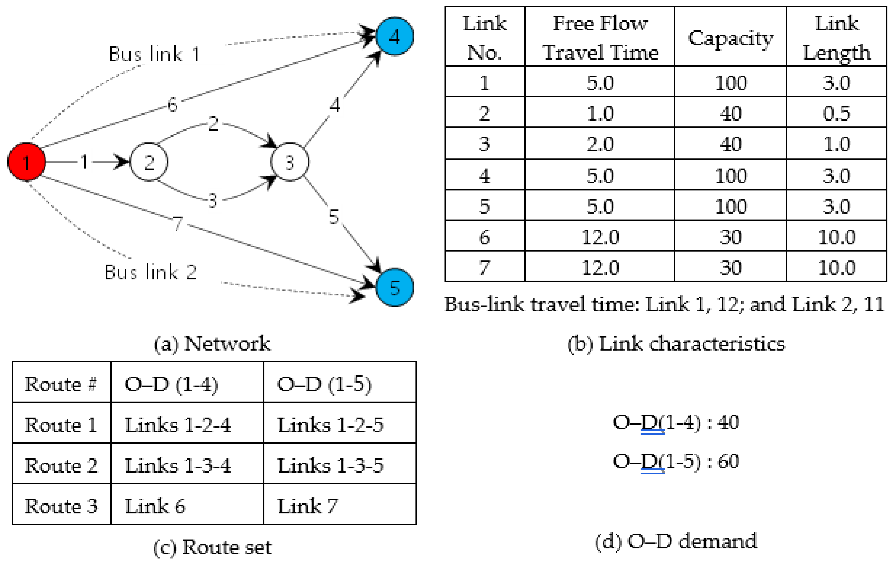
For the numerical experiments, two networks, which are a small network and a real-size network, are used to demonstrate the features of the CMA-EC model and the efficiency of the proposed solution algorithm.

5.1. Small Network

Figure 4 shows the network topology and characteristics of the small network. The network consists of seven links, five nodes, and two O–D pairs (e.g., O–D pairs (1,4) and (1,5)). The standard Bureau of Public Road (BPR) link performance function (alpha = 0.15, beta = 4.00) for link travel time function is used as follows.
t a = t a 0 ( 1 + 0.15 ( v a C a ) 4 ) , a A
The dispersion parameter value of route choice ( θ ) and the dispersion parameter of mode choice ( τ ) are assumed to be 0.2 and 0.1, respectively. To simplify the model, attractiveness ( ψ m r s ) of all modes set as 0. To compute emission values, Equations (2) and (3) for passenger cars are used, and it is assumed that the bus emission is not related to the restriction of car flows, because the number of bus mode usually operates regardless of the number of bus passengers.
First, the effect of imposing the environmental constraints on the CMA problem is shown in Table 1 and Figure 5. Table 1 shows the assigned link flows and total emission value (i.e., TCO = g a m ( x a m ) x a m ) for a passenger car. To gain an idea of the effect of the environmental constraints, it first runs the CMA model without the constraints, and then the environmental constraints are imposed by reducing the emission restriction value from 70 to 20. Table 1 provides a summary of assigned link flows and computed total emission value accordingly. From the table, we can observe that the emission value on Link 1 is higher than other links. In addition, TCO values on Link 5, Link 6, and Link 7 have greater than 30. When the imposed emission value is high (e.g., 70), the link-flow patterns are similar to link flows resulting from without restriction case, because only Link 1 approaches to the restricted value. In contrast, the link-flow patterns show more differences when the emission restricted value is decreased. Specifically, Link 7 and Link 6 are approached to the restricted values after emission-restricted values 60 and 50 are imposed, respectively. Using the results from Table 1, Figure 5 presents the trajectories of total emissions (TCO). When emission restricted values from 70 to 20 are imposed, the TCO pattern is decreased. However, it can observe that TCO values on Link 6 and Link 7 are increased after restriction values 70, 60, and 50 are imposed. When the environmental constraint is imposed on Link 1, the excess flows are diverted to other under-utilized links (e.g., Links 6 and 7) via routes that bypass Link 1. Hence, the flow and emission values on Link 6 and Link 7 are increased. However, other links (e.g., Links 2, 3, 4, and 5) flows and emission values are decreased because these links are directly related to Link 1 in Route 1 and Route 2.
Figure 6 investigates the effects of the environmental constraints on modal splits. The result shows that imposing restricted values 70 and 60 are not sensitive to the modal split in the network (i.e., 1% and 4% increase in the bus mode choice, respectively). On the other hand, the modal split is fairly sensitive when restriction values from 50 to 20 are imposed. When the resection value 50 is imposed, Link 1, Link 6, and Link 7 are approached to the constrained values, and the excess flows are diverted to bus mode, because there are no other under-utilized links in the passenger-car links.
From the test network experiment, we can infer that the excess demand (or restricted demand on vehicles) by the environmental constraints does not change directly to bus demand, because they will find other under-utilized routes. In addition, even if the restriction value is linear, mode-choice change follows a nonlinear pattern.

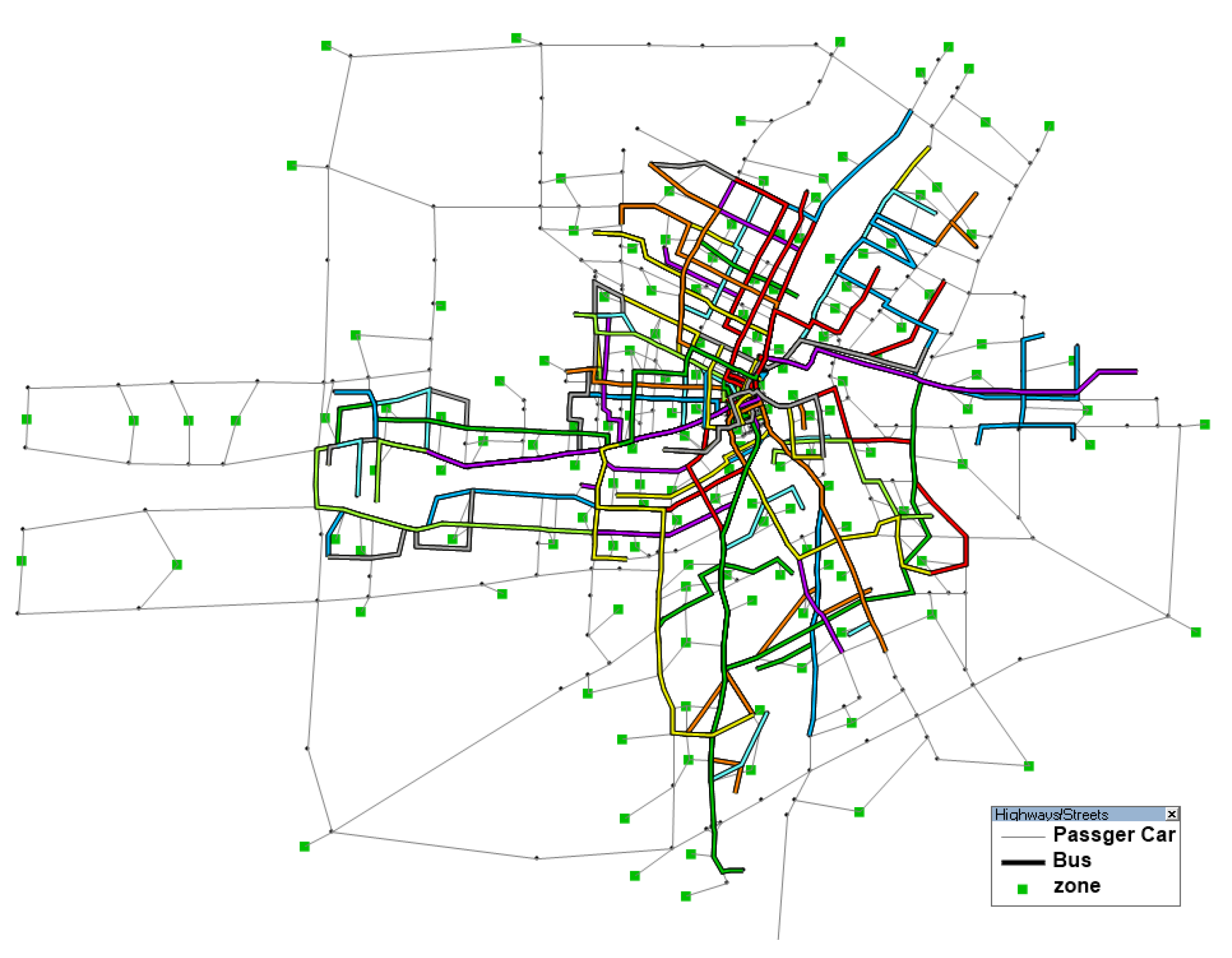
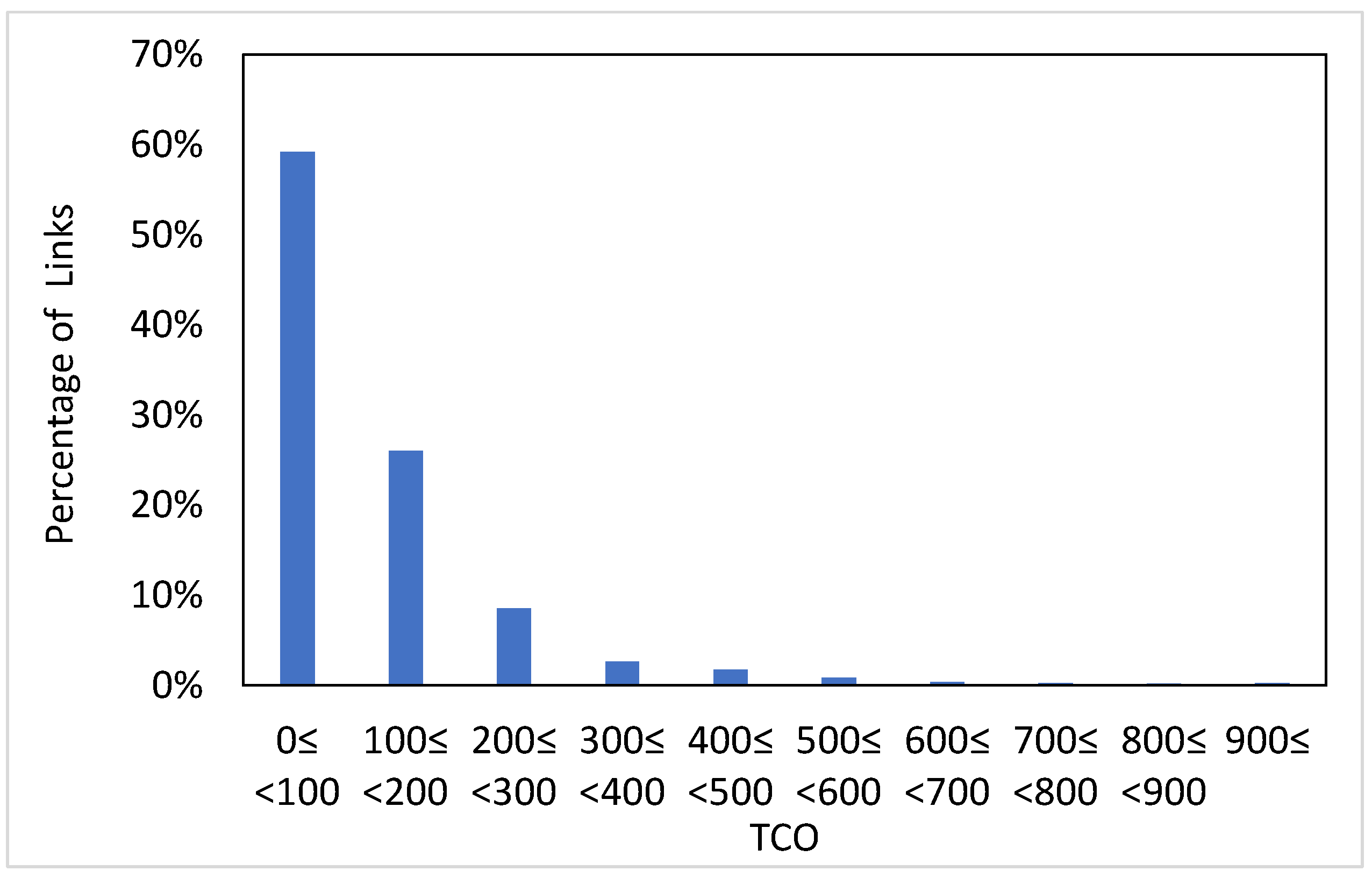
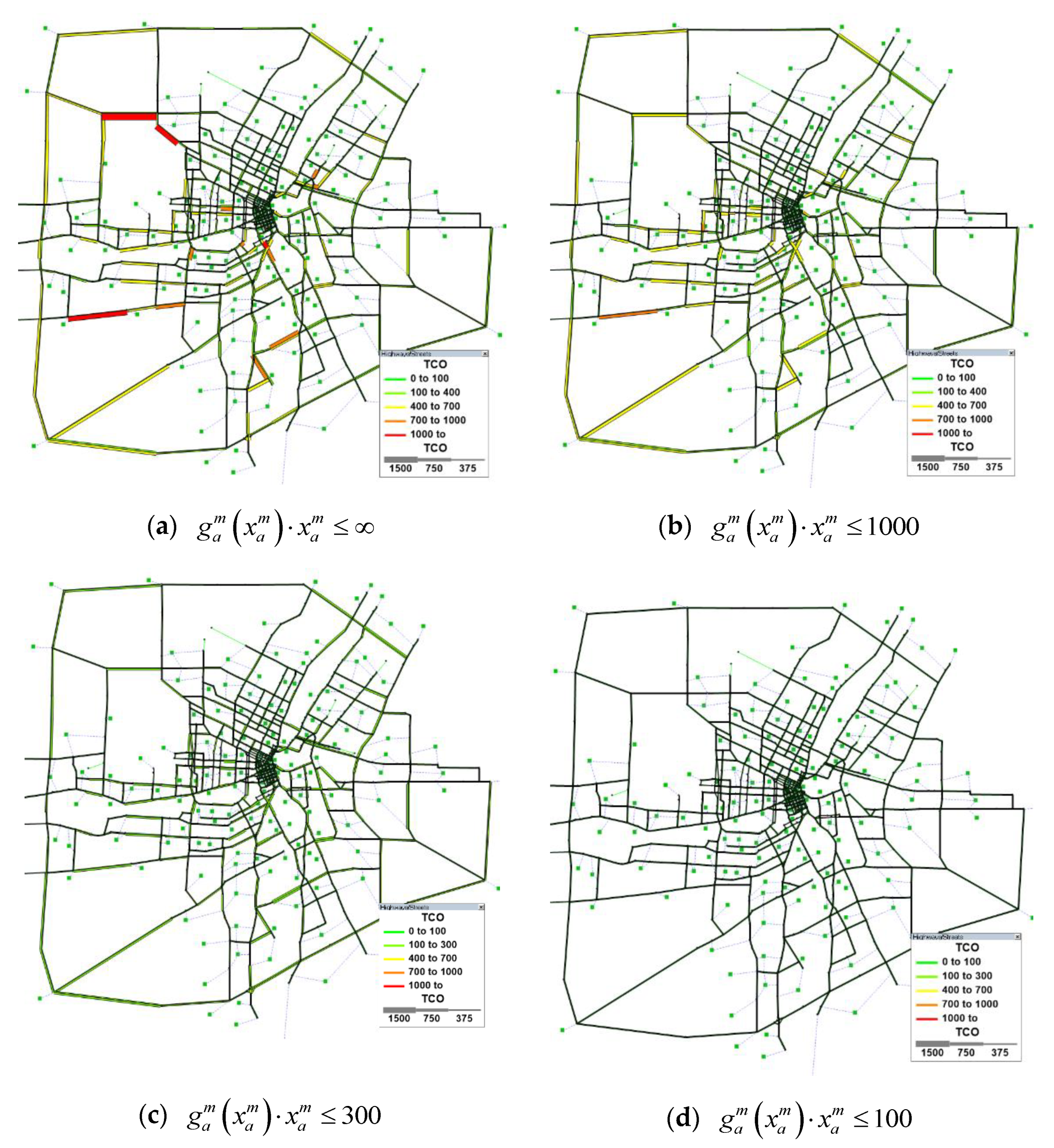
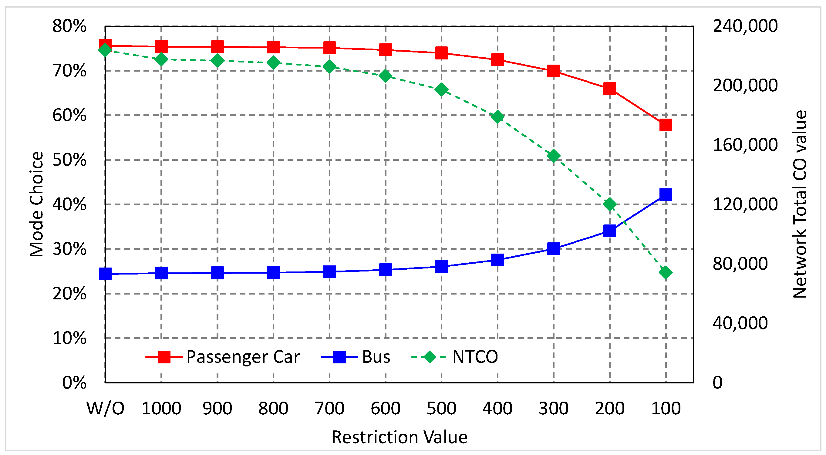
5.2. Winnipeg Network

In this section, numerical experiments, using a real-case study of the Winnipeg network in Canada, are conducted. These experiments are used to examine (a) the convergence characteristics of the proposed iterative balancing algorithm for solving the CMA-EC, (b) link-flow changes with different restriction values, and (c) the mode choice and network total emission change with different restriction values. Similar to the first experiment, the effect of emission on bus demand is not considered, because the number of buses operates regardless of the bus demand. The solution procedure is coded in Intel Visual FORTRAN XE and runs on a 3.60 GHz processor and 64.00 GB of RAM (Santa Clara, CA, USA).
The network, as shown in Figure 7, consists of 154 zones, 2535 links, and 4345 O–D pairs. The network and demand data were obtained from Emme software [55], and route sets (i.e., 174,491 routes) of the network were obtained from Bekhor et al. [56].
First, it runs the CMA model, without the environmental constraints to analyze the current environmental level. Figure 8 shows TCO distribution on all links (i.e., 1932 link, excluding the centroid connectors). From the figure, it can be observed that more than 750 links (40.8%) emitted 100 air pollutants (i.e., TCO > 100). In addition, more than 60 links (3.6%) have a TCO greater than 400.
With Figure 8, the convergence characteristics of the proposed iterative balancing algorithm are shown in Figure 9. From the figure, the proposed algorithm can promise convergence with a Root Mean Square Error (RMSE) of 1 × 10⁻⁸. The total computational effort to reach RMSE of 1 × 10⁻⁸ is less than 12 s (e.g., TCO < 200 case). As decreasing the emission restriction values, computational time grows, because more links are approached to the restricted values.
Figure 10 depicts the TCO values pattern, depending on different imposed restriction values. If no restriction values are applied, it can be observed that several links have higher TCO values (greater than 1000), while the TCO values are gradually decreased after imposing the restriction. Specially, the TCO values pattern is clearly different after imposing 100 values, because passenger-car travelers are diverted to bus mode or other links having lower emissions in their route choice.
Figure 11 shows mode choice change and network total emission (NTCO) change as imposing different restriction values. Based on the figure, we can observe the mode choice is nonlinearly decreased when the imposed restriction values are linearly decreased. When the restriction values from 1000 to 600 are imposed, mode choice is not affected significantly, but after imposing 500 values, the mode-change pattern shows a nonlinearly decreasing pattern. In terms of network total emission values (NTCO), it also shows a decreasing pattern with a decrease of the passenger-car demand, and it is affected more after imposing 500 restriction values, as well. However, from the figure, the NTCO value does not show a linear pattern as the decreasing pattern of passenger-car mode. After imposing 100 values, the mode choice of the passenger car is decreased by about 18%, compared to no-restriction case, while the NTCO values are decreased by about 67%, compared to no-restriction case.
From the real network experiment, it demonstrates that the proposed solution algorithm converged in 30 s. It also showed that the effect of larger restricted values is not significant in an NTCO decrease, but using smaller values has more of an effect (i.e., nonlinearly NTCO decrease).

6. Conclusions

In this paper, an environmental constrained combined modal split and assignment (CMA-EC) model is proposed. A logit-based mode-choice and route-choice model was adopted. Specifically, the iterative balancing algorithm was used for solving CMA, with considerations of the environmental constraints. Using a small and a real network in the city of Winnipeg, Canada, we conducted numerical experiments, to examine the efficiency of the iterative balancing algorithm and the effectiveness of how the environmental constraints affect mode choice and route choice in a multi-modal transportation network. The numerical results revealed that (1) the excess flows are diverted to other under-utilized routes when the environmental constants are imposed, because using passenger cars still has better utility than using a transit. When a traveler chooses a transportation mode, they would consider utilities or benefits (e.g., fare, travel time, and comfortableness). If other routes (e.g., detoured route) have better utilities, the traveler still chooses the passenger car in mode choice. (2) The small restriction value has more efficiency in mode change. When small restriction values are imposed, the utility of the passenger car travelers is decreased, and travelers change their choices to transit modes. (3) The network total emission is reduced in a nonlinear fashion as the number of passenger cars flows. Although the restriction value is linearly decreased, transit travelers are nonlinearly increased. Hence, the network emission is also nonlinearly decreased.
Sustainable transportation planning is receiving great attention. The proposed combined modal split and traffic assignment problem with environmental constraints is useful to determine various environmental protection requirements, such as the environmental cost charging and inducing demand for transit based on air pollution level.
For future research, it would be of interest to (1) impose area-based environmental constraints, (2) further expand public mode (e.g., bus, metro, and bicycle), and (3) consider vehicle interactions with asymmetric cost functions for modes (e.g., passenger car and truck) sharing the same highway network. In addition, the CO emission adopted in this paper can be extendable to other pollutants. Specially, GHG-related emissions (e.g., carbon dioxide (CO2), methane (CH4), nitrous oxide (N2O), and ozone (O3)) can be explored and combined into the proposed model.

Funding

This research was funded by the Basic Science Research Program, grant number NRF-2016R1C1B2016254; and the Ministry of Science, ICT, Republic of Korea, grant number K-21-L01-C05-S01.

Institutional Review Board Statement

Not Applicable.

Informed Consent Statement

Not Applicable.

Data Availability Statement

The data presented in this study are available, upon request, from the corresponding author.

Acknowledgments

The author is grateful to Joonho Ko (guest editor of Sustainability) and three referees for providing constructive comments and suggestions for improving the quality and clarity of the paper.

Conflicts of Interest

The author declare no conflict of interest.

References

  1. EPA (Environmental Protection Agency). U.S. Greenhouse gas Emissions and Sink. 2021. Available online: https://www.epa.gov/sites/production/files/2021-02/documents/us-ghg-inventory-2021-main-text.pdf (accessed on 16 March 2021).
  2. EPA (Environmental Protection Agency). Basic Information about Carbon Monoxide (CO) Outdoor Air Pollution. 2021. Available online: https://www.epa.gov/co-pollution/basic-information-about-carbon-monoxide-co-outdoor-air-pollution (accessed on 16 March 2021).
  3. Kheirbek, I.; Haney, J.; Douglas, S.; Ito, K.; Matte, T. The contribution of motor vehicle emissions to ambient fine particulate matter public health impacts in New York City: A health burden assessment. Environ. Health 2016, 15, 89. [Google Scholar] [CrossRef] [Green Version]
  4. Kim, S. Decomposition analysis of greenhouse gas emissions in Korea’s transportation sector. Sustainability 2019, 11, 1986. [Google Scholar] [CrossRef] [Green Version]
  5. Kyoto Protocol. 1992. Available online: https://en.wikipedia.org/wiki/Kyoto_Protocol (accessed on 14 March 2020).
  6. Paris Agreement. 2016. Available online: https://en.wikipedia.org/wiki/Paris_Agreement (accessed on 14 March 2020).
  7. The Korea Herald. 2019. Available online: https://en.wikipedia.org/wiki/Paris_Agreement (accessed on 18 March 2021).
  8. Reuters. 2018. Available online: https://www.reuters.com/article/us-germany-emissions-factbox-idUSKCN1NK28L (accessed on 18 March 2021).
  9. Auto.com. 2015. Available online: https://auto.economictimes.indiatimes.com/news/passenger-vehicle/cars/ngts-ban-on-diesel-run-vehicles-over-10-years-old-in-delhi-hits-used-cars-hard/46902519 (accessed on 18 March 2021).
  10. The Korea Herald. 2018. Available online: http://www.koreaherald.com/view.php?ud=20180121000206 (accessed on 18 March 2021).
  11. Xu, X.; Chen, A.; Cheng, L. Reformulating environmentally constrained traffic equilibrium via a smooth gap function. Int. J. Sustain. Transp. 2015, 9, 419–430. [Google Scholar] [CrossRef]
  12. Florian, M. A traffic equilibrium model of travel by car and public transit modes. Transp. Sci. 1977, 11, 166–179. [Google Scholar] [CrossRef]
  13. Abdulaal, M.; LeBlanc, L.J. Methods for combining modal split and equilibrium assignment models. Transp. Sci. 1979, 13, 292–314. [Google Scholar] [CrossRef]
  14. Fernandez, E.; de Cea, J.; Floria, M.; Cabrera, E. Network equilibrium models with combined modes. Transp. Sci. 1994, 28, 182–193. [Google Scholar] [CrossRef]
  15. Garcia, R.; Marin, A. Network equilibrium with combined modes models and solution algorithms. Transp. Res. Part B 2005, 39, 223–254. [Google Scholar] [CrossRef]
  16. Ryu, S.; Chen, A.; Choi, K. Solving the combined modal split and traffic assignment problem with two types of transit impedance function. Eur. J. Oper. Res. 2017, 257, 870–880. [Google Scholar] [CrossRef]
  17. Hearn, D.W.; Ribera, J. Bounded flow equilibrium problems by penalty methods. In Proceedings of the IEEE International Conference on Circuits and Computers, New York, NY, USA, 1–3 October 1980. [Google Scholar]
  18. Tam, M.L.; Lam, W.H.K. Maximum car ownership under constraint of road capacity and parking space. Transp. Res. Part A 2000, 34, 145–170. [Google Scholar] [CrossRef]
  19. Tam, M.L.; Lam, W.H.K. Balance for car ownership under user demand and road network supply conditions-case study in Hong Kong. J. Urban Plan. Dev. 2004, 130, 24–36. [Google Scholar] [CrossRef]
  20. Li, Z.C.; Huang, H.J.; Lam, W.H.; Wong, S.C. A model for evaluation of transport policies in multimodal networks with road and parking capacity constraints. J. Math. Model. Algorithms 2006, 6, 239–257. [Google Scholar] [CrossRef]
  21. Ryu, S.; Chen, A.; Xu, X.; Choi, K. A dual approach for solving the combined distribution and assignment problem with link capacity constraints. Netw. Spat. Econ. 2014, 14, 245–270. [Google Scholar] [CrossRef]
  22. Li, Y.; Tan, T.; Li, X. A log-exponential smoothing method for mathematical programs with complementarity constraints. Appl. Math. Comput. 2012, 218, 5900–5909. [Google Scholar] [CrossRef]
  23. Green House Online. 2021. Available online: http://www.ghgonline.org/otherco.htm (accessed on 18 March 2021).
  24. Larsson, T.; Patriksson, M. Side constrained traffic equilibrium models-analysis, computation and applications. Transp. Res. Part B 1999, 33, 233–264. [Google Scholar] [CrossRef] [Green Version]
  25. Bell, M.G.H. Stochastic user equilibrium assignment in network with queues. Transp. Res. Part B 1995, 29, 125–137. [Google Scholar] [CrossRef]
  26. Yang, H.; Lam, W.H.K. Optimal road tolls under conditions of queuing and congestion. Transp. Res. Part A 1996, 30, 319–332. [Google Scholar]
  27. Larsson, T.; Patriksson, M.; Rydegren, C. A column generation procedure for the side constrained traffic equilibrium problem. Transp. Res. Part B 2004, 38, 17–38. [Google Scholar] [CrossRef]
  28. Chen, A.; Zhou, Z.; Ryu, S. Modeling physical and environmental side constraints in traffic equilibrium problem. Int. J. Sustain. Transp. 2011, 5, 172–197. [Google Scholar] [CrossRef]
  29. Ferrari, P. Road pricing and network equilibrium. Transp. Res. Part B 1995, 29, 357–372. [Google Scholar] [CrossRef]
  30. Yang, H.; Bell, M.G.H. Traffic restraint, road pricing and network equilibrium. Transp. Res. Part B 1997, 31, 303–314. [Google Scholar] [CrossRef]
  31. Chen, X.; Kim, I. Modelling rail-based park and ride with environmental constraints in a multimodal transport network. J. Adv. Transp. 2018, 2018, 1–15. [Google Scholar] [CrossRef] [Green Version]
  32. Wallace, C.E.; Courage, K.G.; Hadi, M.A.; Gan, A.G. TRANSYT-7 F User’s Guide; University of Florida: Gainesville, FL, USA, 1988. [Google Scholar]
  33. Yin, Y.; Lawphongpanich, L. Internalizing emission externality on road networks. Transp. Res. Part D 2006, 11, 292–301. [Google Scholar] [CrossRef]
  34. Nagurney, A.; Qiang, Q.; Nagurney, L.S. Environmental impact assessment of transportation networks with degradable links in an era of climate change. Int. J. Sustain. Transp. 2010, 4, 154–171. [Google Scholar] [CrossRef] [Green Version]
  35. Chen, A.; Xu, X. Goal programming approach to solving the network design problem with multiple objectives and demand uncertainty. Expert Syst. Appl. 2012, 39, 4160–4170. [Google Scholar] [CrossRef]
  36. Chen, L.; Yang, H. Managing congestion and emissions on road networks with tolls and rebates. Transp. Res. Part B 2012, 46, 933–946. [Google Scholar] [CrossRef]
  37. Ng, M.W.; Lo, H.K. Regional air quality conformity in transportation networks with stochastic dependencies: A theoretical copula-based model. Netw. Spat. Econ. 2013, 13, 373–397. [Google Scholar] [CrossRef]
  38. Yang, Y.; Yin, Y.; Lu, H. Designing emission charging schemes for transportation conformity. J. Adv. Transp. 2014, 48, 766–781. [Google Scholar] [CrossRef]
  39. Xu, X.; Chen, A.; Cheng, L. Stochastic network design problem with fuzzy goals. Transp. Res. Rec. 2013, 2399, 23–33. [Google Scholar] [CrossRef]
  40. Szeto, W.Y.; Wang, Y.; Wong, S.C. The chemical reaction optimization approach to solving the environmentally sustainable network design problem. Comput. Aided Civ. Infrastruct. Eng. 2014, 29, 140–158. [Google Scholar] [CrossRef] [Green Version]
  41. Boyce, D. Forecasting Travel on congested urban transportation networks: Review and prospects for network equilibrium models. Netw. Spat. Econ. 2007, 7, 99–128. [Google Scholar] [CrossRef]
  42. Yao, J.; Chen, A.; Ryu, S.; Shi, F. A general unconstrained optimization formulation for the combined distribution-assignment problem. Transp. Res. Part B 2014, 59, 137–160. [Google Scholar] [CrossRef]
  43. Tan, H.; Du, M.; Jiang, X.; Chu, Z. The combined distribution and assignment model: A new solution algorithm and its applications in travel demand forecasting for modern urban transportation. Sustainability 2019, 11, 2167. [Google Scholar] [CrossRef] [Green Version]
  44. Wu, Z.X.; Lam, W.H.K. A combined modal split and stochastic assignment model for congested networks with motorized and non-motorized Modes. Transp. Res. Rec. 2003, 1831, 57–64. [Google Scholar] [CrossRef]
  45. Canterella, G.E. A general fixed-point approach to multimode, multiuser equilibrium assignment with elastic demand. Transp. Sci. 1997, 31, 107–128. [Google Scholar] [CrossRef]
  46. Kitthamkesorn, S.; Chen, A.; Xu, X.; Ryu, S. Modeling mode and route similarities in network equilibrium problem with go-green modes. Netw. Spat. Econ. 2016, 16, 33–60. [Google Scholar] [CrossRef]
  47. Florian, M.; Nguyen, S. A combined trip distribution, modal split and trip assignment model. Transp. Res. 1978, 12, 241–246. [Google Scholar] [CrossRef]
  48. Boyce, D.E.; Daskin, M.S. Urban Transportation. In Design and Operation of Civil and Environmental Engineering Systems; ReVelle, C., McGarity, A., Eds.; Wiley: New York, NY, USA, 1997. [Google Scholar]
  49. Wong, K.I.; Wong, S.C.; Wu, J.H.; Yang, H.; Lam, W.H.K. A combined distribution, hierarchical mode choice, and assignment network model with multiple user and mode classes. In Urban and Regional Transportation Modeling; Lee, D.H., Ed.; Edward Elgar Publishing: Cheltnham, UK, 2004; pp. 25–42. [Google Scholar]
  50. Oppenheim, N. Urban Travel Demand Modeling; John Wiley & Sons, Inc.: New York, NY, USA, 1995. [Google Scholar]
  51. Yang, C.; Chen, A.; Xu, X. Improved partial linearization algorithm for solving the combined travel-destination-mode-route choice problem. J. Urban Plan. Dev. 2013, 139, 22–32. [Google Scholar] [CrossRef]
  52. Beckmann, M.J.; McGuire, C.B.; Winsten, C.B. Studies in the Economics of Transportation; Yale University Press: New Haven, CO, USA, 1956. [Google Scholar]
  53. Fisk, C. Some developments in equilibrium traffic assignment. Transp. Res. Part B 1980, 14, 243–255. [Google Scholar] [CrossRef]
  54. Bell, M.G.H.; Iida, Y. Transportation Network Analysis; Wiley: New York, NY, USA, 1997. [Google Scholar]
  55. Emme/4 Software. INRO Consultants, Montréal. 2013. Available online: https://www.inrosoftware.com/ (accessed on 10 March 2014).
  56. Bekhor, S.; Toledo, T. Investigating path-based solution algorithms to the stochastic user equilibrium problem. Transp. Res. Part B 2005, 39, 279–295. [Google Scholar] [CrossRef]
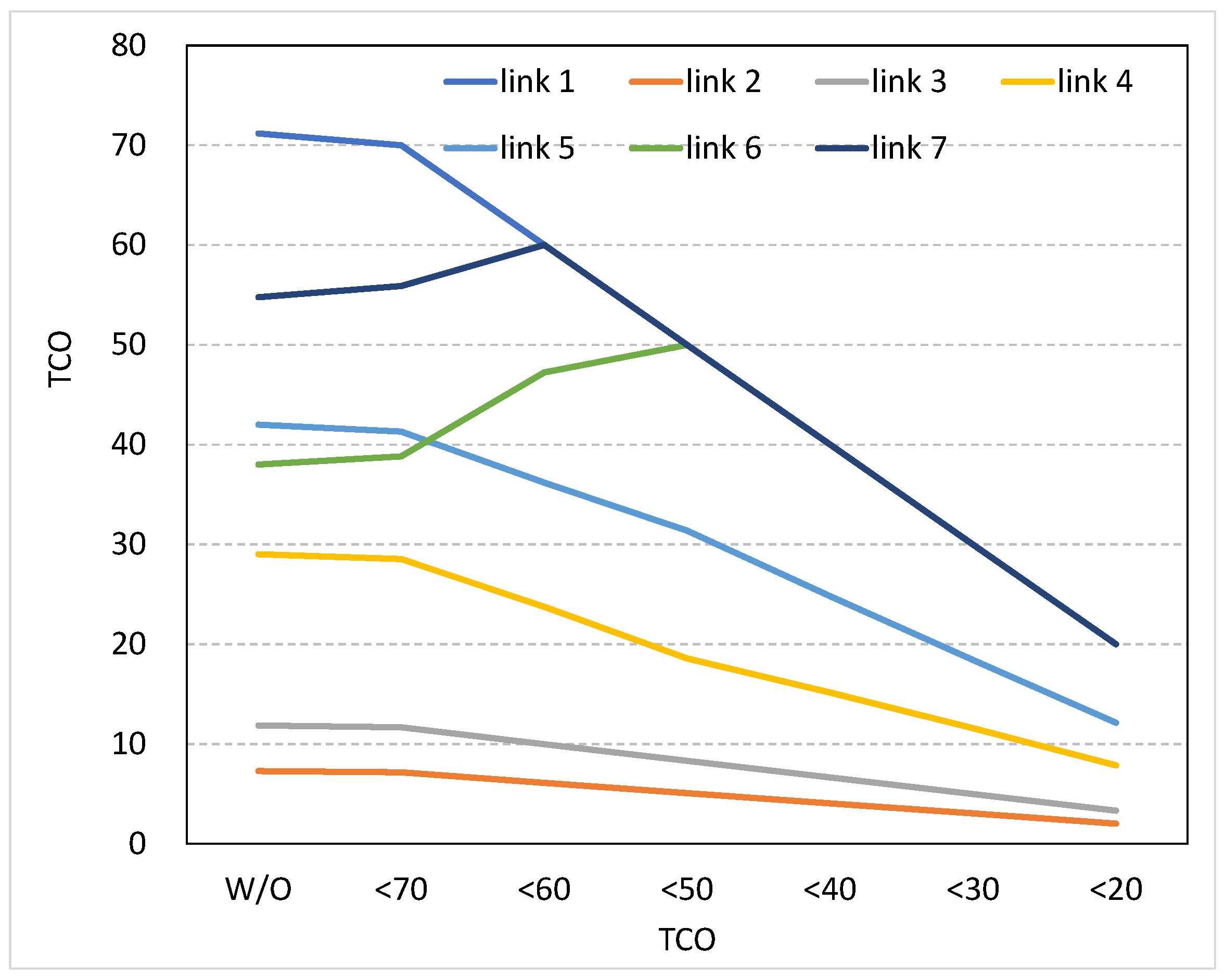
Figure 1. Procedure for combined modal split and traffic assignment (CMA) model with environmental constraints.
Sustainability 13 03780 g001
Figure 2. The Emission-flow curve.
Sustainability 13 03780 g002
Figure 3. Hierarchical structure of the combined mode and route choices.
Sustainability 13 03780 g003
Figure 4. Test network (a) Network, (b) Link characteristics, (c) Route set.
Sustainability 13 03780 g004
Figure 5. Trajectories of total emissions.
Sustainability 13 03780 g005
Figure 6. Effect of environmental restriction on modal splits.
Sustainability 13 03780 g006
Figure 7. Effect of environmental restriction on modal splits.
Sustainability 13 03780 g007
Figure 8. Emitted air-pollutant distribution.
Sustainability 13 03780 g008
Figure 9. Convergence characteristics.
Sustainability 13 03780 g009
Figure 10. Emission-values change map with different restriction values (a) g a m ( x a m ) x a m , (b) g a m ( x a m ) x a m 1000 , (c) g a m ( x a m ) x a m 300 , (d) g a m ( x a m ) x a m 100 .
Sustainability 13 03780 g010
Figure 11. Mode choice and network total emission change with the environmental restriction values.
Sustainability 13 03780 g011
Table 1. Summary of assigned link flows.
ConstraintLink 1Link 2Link 3Link 4Link 5Link 6Link 7
Without constraintFlow43.2023.7519.4517.6525.558.0011.52
TCO71.187.2911.8729.0141.9938.0154.76
TCO 70 Flow42.5023.3619.1317.3725.138.1711.76
TCO70.007.1611.6728.5341.3038.8255.89
TCO 60 Flow36.4720.0516.4214.4522.029.9412.62
TCO60.006.129.9923.7536.1847.2360.00
TCO 50 Flow30.4116.7213.6911.3119.1010.5210.52
TCO50.005.098.3218.5931.3850.0050.00
TCO 40 Flow24.3413.3810.969.2315.118.428.42
TCO40.004.076.6515.1724.8240.0040.00
TCO 30 Flow18.2610.048.227.0511.216.326.32
TCO30.003.054.9911.5918.4130.0030.00
TCO 20 Flow12.176.695.484.787.394.214.21
TCO20.002.033.337.8612.1420.0020.00
Publisher’s Note: MDPI stays neutral with regard to jurisdictional claims in published maps and institutional affiliations.

