
A Lean Approach to Developing Sustainable Supply Chains


Abstract
1. Introduction
- (i)
- (ii)
- Introduces new multi-disciplinary qualitative and quantitative indicators that represent and analyze all facets of sustainability to measure the supply chain performance;
- (iii)
- Through the use of indicators, the whole supply chain is assessed in terms of the three pillars of sustainability. The assessment of materials and information flows between the supply chain actors is performed;
- (iv)
- Identifies, in a quantitative way, the supply chain’s bottlenecks, as well as providing potential solutions, prioritization of actions and recommendations to overcome the identified bottlenecks;
- (v)
- Facilitates creating future value stream maps to attain a (more) sustainable supply chain.
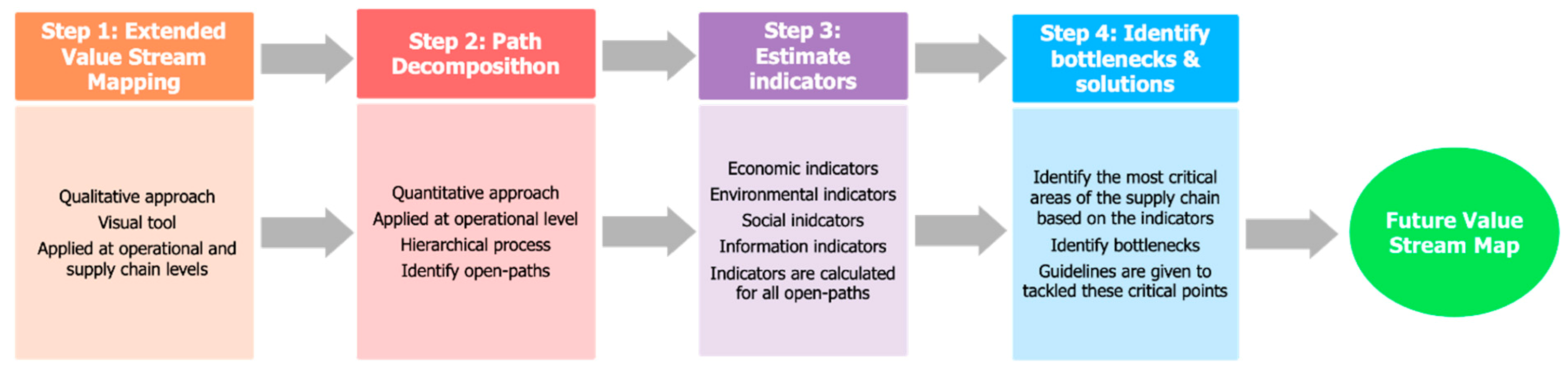
2. Methodology for Lean Design of Sustainable Supply Chains: SustainSC-VSM
2.1. Step 1: Extended Value Stream Mapping (EVSM)
- Factory: (i) average time that the flow spends in the raw materials’ warehouse; (ii) time that the flow is being processed; (iii) time spent in the final goods warehouse; and (iv) the ratio of defects and every part every interval (EPEI).
- Retailer: demand (daily or weekly) for each product of the family.
- Warehouse: (i) ratio of product defects; and (ii) average time that the product flow stays in the warehouse.
2.2. Step 2: Path Decomposition
2.3. Step 3: Calculate Indicators
2.3.1. Step 3.1: Economic Indicators
Cost
Time
Quality
Flexibility
2.3.2. Step 3.2: Environmental Indicators
2.3.3. Step 3.3: Social Indicators
2.3.4. Step 3.4: Information Indicators
2.4. Step 4: Bottleneck Identification and Potential Solutions
3. Results
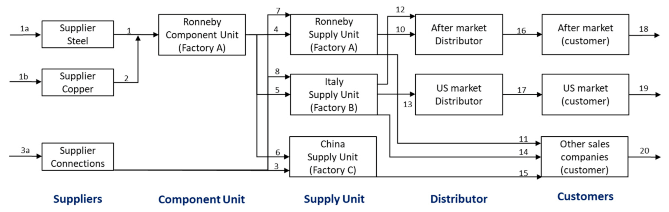
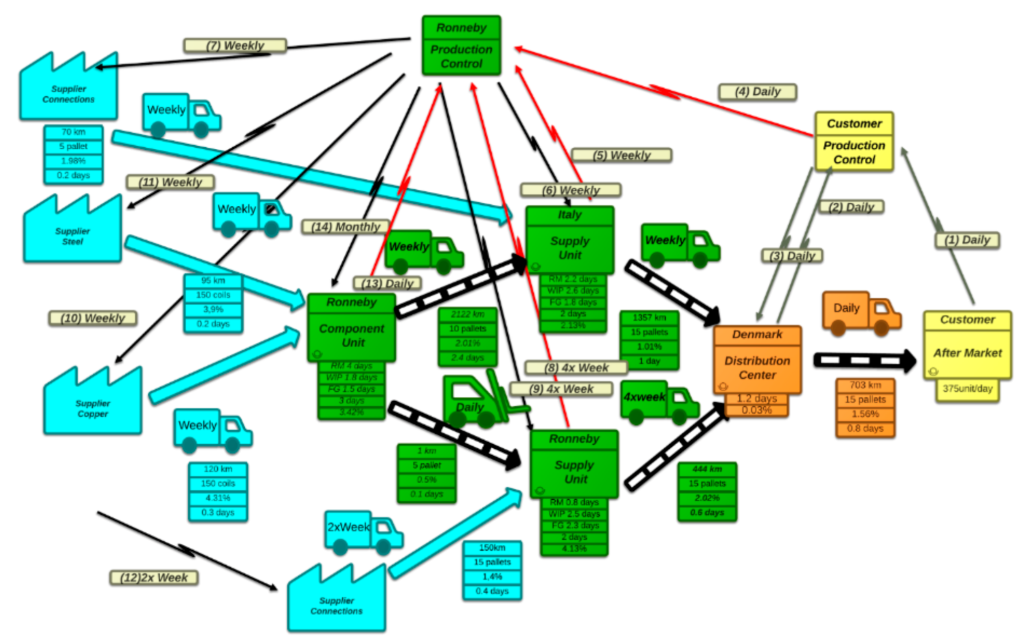
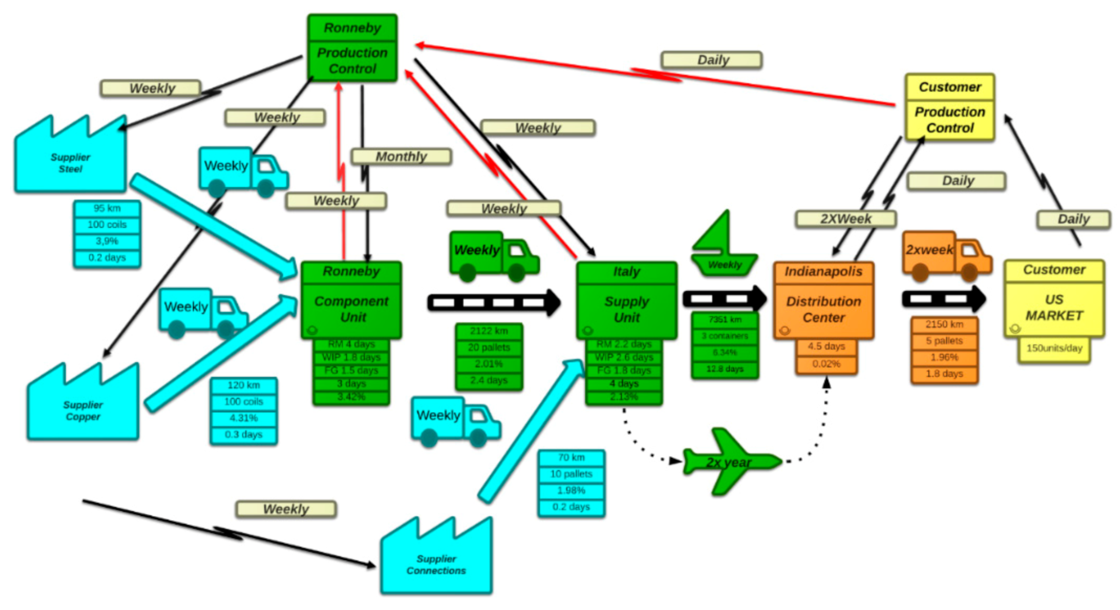
3.1. Step 1: Extended Value Stream Map
- The distances between the different units were obtained by using Google Maps;
- The data needed for the complete description of the data boxes (EPEI, defects, inventory days, batch and demand) of the EVSM were collected from the Alfa Laval sustainability report [67];
- The demand was estimated based on the Alfa Laval sustainability report [67] and by applying some assumptions, such as: (i) the heat exchangers represent 40% of the sales in the equipment divisions, and (ii) the after-market represents 35 % of the total market share.
- The steel and copper suppliers send a weekly shipment of 150 coils to the Ronneby C.U.;
- The component unit is manufactured in the Ronneby C.U.;
- A fraction of the finished items are sent to the Italy S.U. by truck, and the others are sent to the Ronneby S.U. by milk run;
- The heat exchangers are manufactured in each supply unit. The heat exchangers are made of the component unit, which was sent earlier from the Ronneby C.U., and a connection component, which was acquired from a local supplier;
- Once the heat exchangers are manufactured, the supply units’ factories send the finished product to the distribution center in Denmark;
- The finished goods are distributed to all the retailers in the distribution center.
- All retailers send daily information on the sales to the office of customer production control;
- All data are processed in the production control office, and the shipment orders are sent to the distribution center;
- The distribution center sends the shipments’ confirmation back to the office of customer production control;
- The office of customer production control also sends the consumption data and the orders to the production control;
- The information is then processed in Ronneby’s production control office, and orders are sent to the supply units located in Ronneby and Italy;
- The Ronneby and Italy supply units send weekly and daily confirmation of the shipments, respectively;
- The Ronneby production control office also sends daily material requirements to the suppliers;
- The Ronneby production control office sends the monthly production forecast to the Ronneby C.U.
3.2. Step 2: Path Decomposition
3.3. Step 3: Calculation of the Indicators
3.4. Step 4: Bottleneck Identification and Potential Solutions
3.4.1. Economic Indicators
3.4.2. Information Indicators
3.4.3. Environmental Indicators
3.4.4. Social Indicators
- (i)
- It leads to the identification of hot spots (e.g., flow of steel from supplier to the component unit in Ronneby and its transport to the Ronneby supply unit seem to be a critical point due to high levels of inventory);
- (ii)
- It provides suggestions to overcome these hot spots (e.g., change current MTS policy to MTO in order to reduce unnecessary inventory);
- (iii)
- It guides the user towards the development of the future state of the value stream map based on the suggestions provided, allowing the development of a more sustainable supply chain.
4. Conclusions
Author Contributions
Funding
Institutional Review Board Statement
Informed Consent Statement
Data Availability Statement
Conflicts of Interest
Nomenclature
| AF— | Allocation factor [mass or volume allocation] |
| AHP— | Analytic Hierarchy Process |
| BC— | Backorder Cost indicator (EUR) |
| BE— | Bullwhip Effect [ratio] |
| C— | Corruption [Number of lawsuits] |
| Cap— | Capacity |
| CDE— | Carbon Footprint [ton CO2] |
| CE— | Carbon Emissions [ton CO2] |
| C.U.— | Component Unit |
| DDD— | Delivery Due Date |
| Def— | Defective flow |
| Demc— | Demand of compound c |
| Deme— | Demand of Entity e |
| e— | Entity |
| E— | Total number of entities in a given path |
| EC— | Energy Cost [EUR] |
| EDD— | Earliest Due Date |
| EE-VSM— | Energy and Environment VSM |
| EILC— | Entity Inventory Level Cost |
| En— | Energy consumed in each entity of the path |
| EPA— | Environmental Protection Agency |
| EPEI— | Every Part Every Interval |
| EVM— | Environmental VSM |
| EVSM— | Extended Value Stream Map |
| FAR— | Fatal Accident Rate [Event/ (workers*time)] |
| FG— | Finished Goods |
| Fop— | Flow of the open path |
| FTF— | Flexibility Time Factor [ratio] |
| FVF— | Flexibility Volume Factor [ratio] |
| Gen— | Green Energy |
| HC— | Holding Cost |
| Hs— | Highest Salary |
| Inv— | Inventory |
| IT— | Inventory Turn [time units] |
| JIT— | Just in Time |
| KPI— | Key Point Indicator |
| LE— | Labor Equity [ratio] |
| Ls— | Lowest Salary |
| LT— | Lead time |
| LTF— | Lead Time Factor [time units] |
| MVA— | Material Value Added [EUR] |
| MF— | Mass flow |
| Ne— | Number of Employees |
| Ninc— | Number of Incidents |
| Nls— | Number of Lawsuits |
| OLTF— | Operational Lead Time Factor [dimentionless] |
| OEE— | Overall Equipment Efficiency |
| OP— | OK-Parts indicator [%] |
| OTE— | Overall Throughput Effectiveness [%] |
| p— | Path |
| P— | Total number of paths passing in that entity |
| PEx— | Price of the product when leaving the supply chain |
| PEn— | Price of the raw material or the product before the value-added chain |
| PUt— | Price of the utility (fuel, electricity, etc.) [] |
| Rm— | Raw mMaterial |
| SC— | Supply Chain |
| SE— | Sustainable Energy [%] |
| SKU— | Stock Keeping Units |
| SLQF— | Service Level Quantity Factor [dimentionless] |
| SLTF— | Service Level Time Factor [dimentionless] |
| SSCM— | Sustainable Supply Chain Management |
| SMED— | Single Minute Exchange of Dies |
| S.U.— | Supply Unit |
| TFop— | Theoretical Flow of Open path |
| TILC— | Total Inventory Level Cost [EUR] |
| TOC— | Theory of Constraints |
| TPM— | Total Preventive Maintenance |
| VF— | Volume flow |
| VLT— | Variability Lead Time [time units] |
| VSM— | Value Stream Map |
| W— | Waste |
| WF— | Waste Factor [ratio] |
| Wh— | Working Hours |
| WIP— | Work in Progress |
Appendix A. Indicators

| Indicator | Description | Units |
|---|---|---|
| Material Value Added | Value added in the supply chain per path | Euro |
| Energy Cost | The cost of energy consumption per path | Euro |
| Total Inventory Level Cost | The cost of the inventory per path | Euro |
| Entity Inventory Cost | The percentage of cost that represents each entity | Ratio |
| Backorder | The total value of lost sales per path | Euro |
| Lead Time Factor | The total lead time per path | Time |
| Operational Lead Time Factor | The percentage of time that represents each entity | Ratio |
| Inventory Turns | The inventory that takes longer to empty per path | Time |
| Service Level Quantity Factor | The accomplishment of the delivered quantity per path | Ratio |
| Service Level Time Factor | The accomplishment of the delivered time per path | Ratio |
| OK-Parts | The quality of the delivered product per path | Percentage |
| Overall throughout effectiveness | Comparing actual to maximum attainable productivity p.e.p. | Percentage |
| Volume Flexibility | The capacity to adapt to volume demand changes per path | Ratio |
| Time Flexibility | The capacity to adapt to time demand changes per path | Ratio |
| Carbon Emission | The CO2 emissions into the environment per path | Tons CO2 |
| Waste Factor | The disposal of waste material per path | Ratio |
| Sustainable Energy | The ratio of renewable energy used per path | Percentage |
| Labor Equity | The distribution of employee compensation per path | Ratio |
| Fatal Accident Rate | Statistical method that reports the number of incidents per path | Inc/(Em*Time) |
| Corruption | The total number of lawsuits per path | Lawsuits |
| Variability of lead time | The variability of the Lead Time Factor per path | Time |
| Bullwhip Effect | The demand variation of the first entity per path | Ratio |
Appendix B. Data Collection
References
- Tasdemir, C.; Gazo, R. A systematic literature review for better understanding of lean driven sustainability. Sustainability 2018, 10, 2544. [Google Scholar] [CrossRef]
- Dey, M.; LaGuardia, A.; Srinivasan, P. Building Sustainability in Logistics Operations: A Research Agenda. Manag. Res. Rev. 2011, 34, 1237–1259. [Google Scholar] [CrossRef]
- Wilson, L. How to Implement Lean Manufacturing; McGraw-Hill: New York, NY, USA, 2010. [Google Scholar]
- Zakery, A. Logistics Future Trends. In Logistics Operations and Managemen; Elsevier: Amsterdam, The Netherlands, 2011; pp. 93–105. [Google Scholar]
- Battor, M.; Battor, M. The impact of customer relationship management capability on innovation and performance advantages: Testing a mediated model. J. Mark. Manag. 2010, 26, 842–857. [Google Scholar] [CrossRef]
- Stank, R.; Autry, T.; Bell, C.; Gilgor, J.; Petersen, D.; Dittmann, K.; Moon, P.; Tate, M.; Bradley, W. Game-Changing Trends in Supply Chain; Haslam College of Business: Knoxville, TN, USA, 2013. [Google Scholar]
- Council of Supply Chain Management Professionals (CSCMP). Council of Supply Chain Management Professionals—Terms and Glossary; CSCMP: Chicago, IL, USA, 2013. [Google Scholar]
- Vonderembse, M.A.; Uppal, M.; Huang, S.H.; Dismukes, J.P. Designing supply chains: Towards theory development. Int. J. Prod. Econ. 2006, 100, 223–238. [Google Scholar] [CrossRef]
- Linton, J.D.; Klassen, R.; Jayaraman, V. Sustainable supply chains: An introduction. J. Oper. Manag. 2007, 25, 1075–1082. [Google Scholar] [CrossRef]
- Winch, J.K. Supply Chain Management: Strategy, Planning, and Operation. Int. J. Qual. Reliab. Manag. 2003, 20, 398–400. [Google Scholar] [CrossRef]
- Tăucean, I.; Tămășilă, M.; Ivascu, L.; Miclea, Ș.; Negruț, M. Integrating Sustainability and Lean: SLIM Method and Enterprise Game Proposed. Sustainability 2019, 11, 2103. [Google Scholar] [CrossRef]
- Jones, D.T.; Womack, J.P. Seeing the Whole: Mapping the Extended Value Stream; Lean Enterprise Institute: Brookline, MA, USA, 2002. [Google Scholar]
- Carvalho, A.; Matos, H.A.; Gani, R. SustainPro—A tool for systematic process analysis, generation and evaluation of sustainable design alternatives. Comput. Chem. Eng. 2013, 50, 8–27. [Google Scholar] [CrossRef]
- Hartini, S.; Ciptomulyono, U.; Anityasari, M. Extended value stream mapping to enhance sustainability: A literature review. AIP Conf. Proc. 2017, 020030. [Google Scholar] [CrossRef]
- Lindo-Salado-Echeverría, C.; Sanz-Angulo, P.; De-Benito-Martín, J.J.; Galindo-Melero, J. Aprendizaje del Lean Manufacturing mediante Minecraft: Aplicación a la herramienta 5S. RISTI Rev. Ibérica Sist. Tecnol. Inf. 2015. [Google Scholar] [CrossRef]
- Soltero, C.; Waldrip, G. Using Kaizen to Reduce Waste and Prevent Pollution. Environ. Qual. Manag. 2002, 11, 23–38. [Google Scholar] [CrossRef]
- Womack, J.P. Value stream mapping. Manuf. Eng. 2006, 136, 145. [Google Scholar]
- Haefner, B.; Kraemer, A.; Stauss, T.; Lanza, G. Quality Value Stream Mapping. Procedia CIRP 2014, 17, 254–259. [Google Scholar] [CrossRef]
- McKellen, C. Pull and kanbans [production control]. Metalwork. Prod. 2004, 148, 16. [Google Scholar]
- Biotto, C.; Mota, B.; Araújo, L.; Barbosa, G.; Andrade, F. Adapted use of andon in a horizontal residential construction project. In Proceedings of the 22nd Annual Conference of the International Group for Lean Construction: Understanding and Improving Project Based Production, Oslo, Norway, 25–27 June 2014; pp. 1295–1605. [Google Scholar]
- Jain, A.; Bhatti, R.; Singh, H. Total productive maintenance (TPM) implementation practice. Int. J. Lean Six Sigma 2014, 5, 293–323. [Google Scholar] [CrossRef]
- Rahayu, A. Implementasi Single Minute Exchange of Dies (Smed) Untuk Perbaikan Proses Brand Changeover Mesin Focke Dan Protos. Ind. Xplore 2020, 5, 8–16. [Google Scholar] [CrossRef]
- Talekar, A.A.; Patil, S.Y.; Shinde, P.S.; Waghmare, G.S. Setup time reduction using single minute exchange of dies (SMED) at a forging line. AIP Conf. Proc. 2019, 020018. [Google Scholar] [CrossRef]
- Da Silva, M.G. Jidoka: Concepts and application of autonomation in an electronics industry company. Espacios 2016, 37. [Google Scholar]
- Rothenberg, S.; Pil, F.K.; Maxwell, J. Lean, green, and the quest for superior environmental performance. Prod. Oper. Manag. 2001, 10, 228–243. [Google Scholar] [CrossRef]
- Faulkner, W.; Badurdeen, F. Sustainable Value Stream Mapping (Sus-VSM): Methodology to visualize and assess manufacturing sustainability performance. J. Clean. Prod. 2014, 85, 8–18. [Google Scholar] [CrossRef]
- Mishra, A.K.; Sharma, A.; Sachdeo, M.; Jayakrishna, K. Development of sustainable value stream mapping (SVSM) for unit part manufacturing. Int. J. Lean Six Sigma 2019, 11, 493–514. [Google Scholar] [CrossRef]
- Djatna, T.; Prasetyo, D. Integration of Sustainable Value Stream Mapping (Sus. VSM) and Life-Cycle Assessment (LCA) to Improve Sustainability Performance. Int. J. Adv. Sci. Eng. Inf. Technol. 2019, 9, 1337. [Google Scholar] [CrossRef]
- Ikatrinasari, Z.F.; Hasibuan, S.; Kosasih, K. The Implementation Lean and Green Manufacturing through Sustainable Value Stream Mapping. IOP Conf. Ser. Mater. Sci. Eng. 2018, 453, 012004. [Google Scholar] [CrossRef]
- Muñoz-Villamizar, A.; Santos, J.; Garcia-Sabater, J.J.; Lleo, A.; Grau, P. Green value stream mapping approach to improving productivity and environmental performance. Int. J. Product. Perform. Manag. 2019, 68, 608–625. [Google Scholar] [CrossRef]
- Torres, A.S.; Gati, A.M. Environmental Value Stream Mapping (EVSM) as sustainability management tool. In Proceedings of the PICMET ’09—2009 Portland International Conference on Management of Engineering & Technology, Portland, OR, USA, 2–6 August 2009; pp. 1689–1698. [Google Scholar] [CrossRef]
- Verma, N.; Sharma, V. Energy Value Stream Mapping a Tool to Develop Green Manufacturing. Procedia Eng. 2016, 149, 526–534. [Google Scholar] [CrossRef]
- Dombrowski, U.; Riechel, C.; Ernst, S. Energy Value Stream Mapping as a Tool of the Digital Factory—Sustainable Optimization with Simulative Energy Value Stream Mapping. Ind. Manag. 2012, 55–58. [Google Scholar]
- United States Environmental Protection Agency (EPA). The Lean & Energy Toolkit; EPA: Washington, DC, USA, 2019. [Google Scholar]
- United States Environmental Protection Agency (EPA). The Lean and Environment Toolkit; EPA: Washington, DC, USA, 2007. [Google Scholar]
- Carvalho, A.; Gani, R.; Matos, H. Design of sustainable chemical processes: Systematic retrofit analysis generation and evaluation of alternatives. Process Saf. Environ. Prot. 2008, 86, 328–346. [Google Scholar] [CrossRef]
- Carvalho, A.; Gani, R.; Matos, H. Design of Sustainable Chemical Processes: Systematic Retrofit Analysis, Generation and Evaluation of Alternatives; Instituto Superior Tecnico: Lisbon, Portugal; Denmark Technical University: Copenhagen, Denmark, 2009. [Google Scholar]
- Mah, R.S. Application of graph theory to process design and analysis. Comput. Chem. Eng. 1983, 7, 239–257. [Google Scholar] [CrossRef]
- Beamon, B.M. Measuring supply chain performance. Int. J. Oper. Prod. Manag. 1999, 19, 275–292. [Google Scholar] [CrossRef]
- Shepherd, C.; Günter, H. Measuring supply chain performance: Current research and future directions. Int. J. Product. Perform. Manag. 2006, 55, 242–258. [Google Scholar] [CrossRef]
- Bolstorff, P. Measuring the impact of supply chain performance. CLO Chief Logist. Off. 2003, 12, 11. [Google Scholar]
- Gunasekaran, A.; Patel, C.; McGaughey, R.E. A framework for supply chain performance measurement. Int. J. Prod. Econ. 2004, 87, 333–347. [Google Scholar] [CrossRef]
- Angerhofer, B.J.; Angelides, M.C. A model and a performance measurement system for collaborative supply chains. Decis. Support Syst. 2006, 42, 283–301. [Google Scholar] [CrossRef]
- Jammernegg, W.; Reiner, G. Performance improvement of supply chain processes by coordinated inventory and capacity management. Int. J. Prod. Econ. 2007, 108, 183–190. [Google Scholar] [CrossRef]
- U.S. Department of Transportation. US Department of Transportation, 2002; U.S. Department of Transportation: Washington, DC, USA, 2002.
- Ye, T. Inventory management with simultaneously horizontal and vertical substitution. Int. J. Prod. Econ. 2014, 156, 316–324. [Google Scholar] [CrossRef]
- Liao, T.W.; Chang, P.C. Impacts of forecast, inventory policy, and lead time on supply chain inventory—A numerical study. Int. J. Prod. Econ. 2010, 128, 527–537. [Google Scholar] [CrossRef]
- Lee, H.L.; Padmanabhan, V.; Whang, S. Information Distortion in a Supply Chain: The Bullwhip Effect. Manag. Sci. 2004, 50, 1875–1886. [Google Scholar] [CrossRef]
- Rother, M.; Shook, J. Lean Enterprise Institute. In Learning to See: Value Stream Mapping to Create Value and Eliminate Muda; Lean Enterprise Institute: Boston, MA, USA, 2003. [Google Scholar]
- Soltani, E.; Azadegan, A.; Liao, Y.Y.; Phillips, P. Quality performance in a global supply chain: Finding out the weak link. Int. J. Prod. Res. 2011, 49, 269–293. [Google Scholar] [CrossRef]
- Giri, B.C.; Sharma, S. Optimizing a closed-loop supply chain with manufacturing defects and quality dependent return rate. J. Manuf. Syst. 2015, 35, 92–111. [Google Scholar] [CrossRef]
- Buchmeister, B.; Friscic, D.; Lalic, B.; Palcic, I. Analysis of a Three-Stage Supply Chain with Level Constraints. Int. J. Simul. Model. 2012, 11, 196–210. [Google Scholar] [CrossRef]
- Muthiah, K.M.N.; Huang, S.H. Overall throughput effectiveness (OTE) metric for factory-level performance monitoring and bottleneck detection. Int. J. Prod. Res. 2007, 45, 4753–4769. [Google Scholar] [CrossRef]
- Nakajima, S. Introduction to TPM: Total Productive Maintenance; Productivity Press: Boca Raton, FL, USA, 1988. [Google Scholar]
- Das, S.K.; Abdel-Malek, L. Modeling the flexibility of order quantities and lead-times in supply chains. Int. J. Prod. Econ. 2003, 85, 171–181. [Google Scholar] [CrossRef]
- Chaabane, A.; Ramudhin, A.; Paquet, M. Design of sustainable supply chains under the emission trading scheme. Int. J. Prod. Econ. 2012, 135, 37–49. [Google Scholar] [CrossRef]
- Mimoso, A.F.; Carvalho, A.; Mendes, A.N.; Matos, H.A. Roadmap for Environmental Impact Retrofit in chemical processes through the application of Life Cycle Assessment methods. J. Clean. Prod. 2015, 90, 128–141. [Google Scholar] [CrossRef]
- Mintcheva, V. Indicators for environmental policy integration in the food supply chain (the case of the tomato ketchup supply chain and the integrated product policy). J. Clean. Prod. 2005, 13, 717–731. [Google Scholar] [CrossRef]
- Popovic, T.; Barbosa-Póvoa, A.; Kraslawski, A.; Carvalho, A. Quantitative indicators for social sustainability assessment of supply chains. J. Clean. Prod. 2018, 180, 748–768. [Google Scholar] [CrossRef]
- Hutchins, M.J.; Sutherland, J.W. An exploration of measures of social sustainability and their application to supply chain decisions. J. Clean. Prod. 2008, 16, 1688–1698. [Google Scholar] [CrossRef]
- Roberts, S.E. Britain’s most hazardous occupation: Commercial fishing. Accid. Anal. Prev. 2010, 42, 44–49. [Google Scholar] [CrossRef] [PubMed]
- Sabato, M.; Bruccoleri, L. The Relationship between Bullwhip Effect and Lead Times Variability in Production—Distribution Networks. 2005. Available online: https://pure.unipa.it/it/publications/the-relationship-between-bullwhip-effect-and-lead-times-variabili-2 (accessed on 1 March 2021).
- Chen, F.; Drezner, Z.; Ryan, J.K.; Simchi-Levi, D. Quantifying the bullwhip effect in a simple supply chain: The impact of forecasting, lead times, and information. Manag. Sci. 2000, 46, 436–443. [Google Scholar] [CrossRef]
- Persson, F. SCOR template—A simulation based dynamic supply chain analysis tool. Int. J. Prod. Econ. 2011, 131, 288–294. [Google Scholar] [CrossRef]
- Bradstreet, D. ALFA LAVAL SPA Company Profile. 2021. Available online: https://www.dnb.com/business-directory/company-profiles.alfa_laval_spa.501f128743daf278bb2b98eafd02e422.html (accessed on 1 March 2021).
- AlfaLaval. Alfa Laval Partner Days. 2018. Available online: https://www.alfalaval.com/globalassets/images/misc/partnerdays/alfalavalpartnerdays2018-programme.pdf (accessed on 1 March 2021).
- Alfa Laval. Alfa Laval Sustainability GRI Report; Alfa Laval: Lund, Sweden, 2014. [Google Scholar]
- Lucidchart. “Lucidchart.” © 2021 Lucid Software Inc. 2021. Available online: https://www.lucidchart.com/pages/examples/value-stream-mapping-software (accessed on 1 March 2021).
- Carvalho, A.; Matos, H.A.; Gani, R. Design of batch operations: Systematic methodology for generation and analysis of sustainable alternatives. Comput. Chem. Eng. 2009, 33, 2075–2090. [Google Scholar] [CrossRef]
- Davis, S.C.; Boundy, R.G. Transportation Energy Data Book, 39th ed.; Oak Ridge National Laboratory, U.S. Department of Energy, Office of Science: Oak Ridge, TN, USA, 2021. [Google Scholar]


| Tool | References | Brief Description |
|---|---|---|
| 5S | [15] |
|
| Kaizen | [16] |
|
| VSM | [17,18] |
|
| Extended VSM (EVSM) | [12] |
|
| Kanban and Visual Factory | [19] |
|
| Visual Management (Andon) | [20] |
|
| Total Productive Maintenance(TPM) | [21] |
|
| Single Minute Exchange of Dies (SMED) | [22,23] |
|
| Jidoka (Autonomation) | [24] |
|
| Just-in-time (JIT) | [25] |
|
| Sustainable-VSM | [26,27,28,29] |
|
| Green VSM | [30] |
|
| Environmental VSM | [31] |
|
| Energy Value Stream Mapping | [32,33] |
|
| EPA Lean and Energy Toolkit | [34] |
|
| EPA Lean and Environment Toolkit | [35] |
|
| Data | ||
|---|---|---|
| Entity | Path | |
| Factory/Warehouse | Transport | |
| Price Utility | Price Utility | Price Product |
| Energy Consumption | Energy Consumption | Price Raw Material |
| Inventory | Lead Time | Costumer Demand |
| Holding Cost | Defective Flow | On Time |
| Lead Time | Carbon Footprint | Theoretical Flow |
| Demand | Green Energy Consumption | Due Date for Delivery |
| Defective Flow | Number of Incidents | Earliest Due Date |
| Process Capacity | Employees | Variance of Lead Time |
| Carbon Footprint | Number of Lawsuits | Variance of Demand |
| Waste | Waste | Variance of Mass Flow |
| Green Energy Consumption | Lower Salary | Penalty Rate |
| Number Incidents | Higher Salary | |
| Employees | Working Hours per Year | |
| Number of Lawsuits | ||
| Demand Downstream Entity | ||
| Lower Salary | ||
| Higher Salary | ||
| Working Hours per Year | ||
| Indicator | Description | Reference | Equation | Nomenclature | |
|---|---|---|---|---|---|
| Material Value Added–SC (MVA-SC) | MVA-SC estimates the value generated between the start and the endpoint of a given path. This indicator is expressed in EUR, and, consequently, negative values of MVA-SC identify the need for changes/improvements. | Adapted from [36] to the supply chain context | Equation (1) | Fop—flow open path (kg/h) PEX—final product selling price PEN—price of raw material | |
| Energy Cost-SC (EC-SC) | EC-SC provides the value of energy consumption in a certain path. AF specifies the allocation of the energy consumed per path, estimated in mass or volume according to Equations (3) and (4). As expected, having high values of EC-SC indicates the need for changes/improvements. | Adapted from [36] to the supply chain context | Equation (2) | e—entity Put—price of utility Ene—energy consumed in each entity of the path AFe—allocation factor of the energy consumed MF—mass flow VF—volume flow | |
| Equation (3) | |||||
| Equation (4) | |||||
| Total Inventory Level Cost (TILC) | Inventory is needed to buffer market and operational uncertainties; however, it often hides inefficient management of supply chain processes. This potentially leads to damages to the supply chain competitiveness due to unnecessary and avoidable costs [44]. The inventory cost represents 33% of the logistics cost [45]. To keep track of this, the Total Inventory Level Factor (TILC) indicator provides information about the most critical paths with regard to inventory costs. When keeping more inventory than necessary, the TILC will present high values, which points out excess costs in this regard. | Developed in this work | Equation (5) | Inve—inventory of entity e HCe—holding cost of a given SKU and entity e | |
| Entity Inventory Level Cost (EILC) | EILC specifies which entity (or entities) is (are) the most critical in inventory cost, within the identified critical path identified previously by TILC. The closer to 1, the worst the entity performs in terms of inventory costs. | Developed in this work | Equation (6) | (see nomenclature given in indicator TILC) | |
| Backorder Cost (BC) | Running out of stock potentially leads to the company losing the order. Furthermore, a poor service level might lead the customers to change to a competing company [46]. Hence, monitoring these losses is critical, and this can be achieved by using the BC indicator, which displays the total value of lost sales in a given path. The price of the product suffers an increment due to client compensation. High BC points out inefficiencies. | Developed in this work | Equation (7) | C—demand of component c Demc—demand of component c | |
| Indicator | Description | Reference | Equation | Nomenclature | |
|---|---|---|---|---|---|
| Lead Time Factor (LTF) | LTF gives the total lead time of each path. It aims at identifying the critical paths with regard to lead time, which can more easily contribute to a service level problem. High values indicate the need for improvements. | Adapted from [37] to the supply chain context | Equation (8) | LT—lead time of entity e | |
| Operational Lead Time Factor (OLTF) | OLTF identifies the most critical entity (or entities) within the critical paths pointed out by LTF. High values indicate potential bottlenecks with regard to the entity’s lead time. | Adapted from [37] to the supply chain context | Equation (9) | (see nomenclature given in indicator LTF) | |
| Inventory Turnover (IT) | IT indicator is used to indicate which inventory takes the longest to empty in a given path. It is only applied to entities with an inventory. High values of IT indicate high lead time, which points to lower agility of the path, and the more noticeable the bullwhip effect. | Adapted from [12] to the supply chain context | Equation (10) | Deme—demand of the downstream process in considered time period Inve—largest inventory of entity e | |
| Indicator | Description | Reference | Equation | Nomenclature | |
|---|---|---|---|---|---|
| Service Level Quantity Factor (SLQF) | To keep track of the orders and the product demand quantities, SLQF informs if the orders are being fully satisfied in terms of the amount. When different from 0, it reports that the service level in terms of quantity is not at its best—that path is not satisfying the customer and thus needs to be improved. | Developed in this work | Equation (11) | (see nomenclature given in indicators BC and MVA-SC) | |
| Service Level Time Factor (SLTF) | Like SLQF, the SLTF indicator informs about the time as a service level by comparing the actual product delivery time to the expected/planned delivery time specified in the order. Values different from 0 indicate that the path’s service level in terms of timely delivery needs improvement. | Developed in this work | Equation (12) | OnTime—flowrate of the open path delivered according to the scheduled time (see nomenclature given in indicator MVA-SC) | |
| OK-Parts (OP) | OP keeps track and raises awareness of the defected products in the value stream. It gives the ratio of product flow that successfully reaches the costumers with a suitable quality compared to the total amount produced. The lower the OP value, the worse the quality performance of the path. | Developed in this work | Equation (13) | Defe—defective flowrate of entity e (see nomenclature given in indicators EC-SC and MVA-SC) | |
| Overall Throughput Effectiveness (OTE-SC) | To go a step further, in this work, we propose the OTE-SC metric to compare actual productivity to the maximum achievable productivity for a given path. Low values of OTE-SC indicate low production performance and the need to improve the production yield. | Adapted from [53] to the supply chain context | Equation (14) | TFop—theoretical flow of an open path working at full yield (see nomenclature given in indicators EC-SC and MVA-SC) | |
| Indicator | Description | Reference | Equation | Nomenclature | |
|---|---|---|---|---|---|
| Flexibility Volume Factor (FVF) | FVF assesses if the company can adapt its production to demand variation in terms of quantity. Low values of FVF indicate a low capacity to adjust production to demand variations. | Developed in this work | Equation (15) | Cape—process capacity of the entity e of a given path (see nomenclature given in indicator IT) | |
| Flexibility Time Factor (FTF) | FTF quantifies the company’s capability to adapt production to meet demand changes regarding time. The lower the value of FTF, the lower the company’s capacity to respond to changes in deadlines. | Adapted from [39] to the supply chain context | Equation (16) | DDD—due date for delivery EDD—earliest due date for which delivery can be made (see nomenclature given in indicator LTF) | |
| Indicator | Description | Reference | Equation | Nomenclature | |
|---|---|---|---|---|---|
| Carbon Emissions (CE) | CE quantifies the CO2 emissions for each open path. High values of CE indicate the need to adopt more energy-efficient equipment and facilities and/or optimize the supply chain operations. | Developed in this work | Equation (17) | CDEe—carbon dioxide emissions emitted by entity e (see nomenclature given in indicator EC-SC) | |
| Waste Factor (WF) | WF measures the material waste disposal in the open paths. High values of WF point out a need for improvements and potential opportunities to reduce waste of resources and reduce operating costs by increasing material recycling. | Developed in this work | Equation (18) | We—material waste from entity e (see nomenclature given in indicators MVA-SC and EC-SC) | |
| Sustainable Energy (SE) | To motivate companies to commit to using more sustainable energy sources, SE measures the ratio of sustainable energy on the total energy consumed in the supply chain operations. The lower the ratio, the higher the need to adopt more environmentally friendly sources of energy. | Adapted from [58] to the supply chain context | Equation (19) | Gene—consumption of green energy by entity e Ene—consumption of energy by entity e (see nomenclature given in indicator EC-SC) | |
| Indicator | Description | Reference | Equation | Nomenclature | |
|---|---|---|---|---|---|
| Labor Equity (LE) | To assess the labor market, LE describes the distribution of employee compensation. The closer the LE ratio is to one, the better the distribution of equity. | Adapted from [60] to the supply chain context | Equation (20) | LSe—lowest salary of a given entity e HSe—highest salary of a given entity e including all benefits | |
| Fatal Accident Rate (FAR) | FAR is a statistical method that reports the number of fatal incidents [61] of an activity based upon the total number of employees working their entire lifetime. The higher the FAR, the bigger the need to improve procedures and/or change the operations. FAR was firstly proposed by the British chemical industry and here adjusted to the supply chain context. | Adapted from [61] to the supply chain context | Equation (21) | Nince—number of incidents in entity e NEe—number of employees that work in entity e Whe—working hours per year in entity e | |
| Corruption (C) | C is an attempt to quantify the effect of corruption on the social sustainability of an enterprise. The higher the C, the greater the need to change policies to fight corruption [59]. | Developed in this work | Equation (22) | Nlse—number of lawsuits in entity e | |
| Indicator | Description | Reference | Equation | Nomenclature | |
|---|---|---|---|---|---|
| Variability of Lead Time (VLT) | VLT aims at monitoring the lead time variability. High values indicate the need to improve the information flow’s stability across a given path within the supply chain. | Developed in this work | Equation (23) | —standard deviation of the lead time factor of a given path LTF—lead time factor of a given path | |
| Bullwhip Effect (BE) | BE gives information concerning the demand variation in the more upstream process of a certain path to promote information sharing and prevent the bullwhip effect. The original equation used to quantify the bullwhip magnitude has been adapted to fit with the open path context. Since the more considerable order quantity variations are located in the most upstream process [48], each path only focuses on the demand increase of the first entity considered in the analysis. | Adapted from [63] to the open path context | Equation (24) | —variance of the orders of the first entity of a given path —demand of flow of a given path | |
| Indicator | Recommendations |
|---|---|
| MVA-SC | Redesign the production process, for example, by applying process intensification and/or process integration. |
| EC-SC | Invest in equipment and vehicles that are more efficient, as well as investing in continuous heat integration. |
| TILC EILC | Decrease the level of production and demand uncertainty. The production uncertainty can be reduced by implementing more robust production processes. Demand uncertainty can be decreased by identifying a significant buffer near the end customer to protect the supply chain from market uncertainties or by applying a production leveling technique (“heijuka”). |
| BC | Improve supply chain coordination and inventory management policies. |
| LTF OLTF | Ideally, all activities should be located at the same place near the end customer. This is often not possible, so the recommendation is to find facilities that share material flows and locate them as close as possible. Using “just in time” methods such as pull systems or process synchronization also shortens the lead time. |
| IT | Reduce the inventory by gradually ensuring not compromising the service level or reducing the batches’ size and increasing the pick-up frequency. |
| VF TF | Redirect the flow of material to another path with a lower workload, or boost the work capacity acquiring newer and more effective equipment. |
| OK-P | Implement failure prevention techniques (“poka yoke”) to reduce scrap and rework in every facility’s production processes. |
| SLQF SLTF | Improve the information sharing between the supply chain members to know the capacity constraints and each supplier’s inventory management. According to the collected information, find out how to deliver the required orders in the proper quantity and time. |
| OTE-SC | Implement kaizen workshops to decrease the production uncertainty (technical, organizational and quality losses, and changeover times). |
| VLT | Homogenize all the processes of the value stream to gain stability and ensure consistent results over time. |
| BE | Adopt a centralized multi-echelon inventory control system since it presents a superior performance over independently operating site-based inventory. |
| CE | Implement more energy-efficient equipment, vehicles and facilities; and/or optimize the supply chain operations. |
| WF | Reengineer the production process to be more efficient and promote recycling policies. |
| SE | Improve energy efficiency and invest in renewable and sustainable energy sources. |
| LE | Improve the lowest salary and/or reduce the highest salary—decrease salary disparity. |
| FAR | Improve labor conditions by implementing robust security policies and provide training to the employees. |
| C | Organize workshops to raise awareness among managers and promote transparent communication of information. |
| Data Boxes | TIME | Total | EPEI | Defects | Steps | |||
|---|---|---|---|---|---|---|---|---|
| Rm (Days) | WIP (Days) | FG (Days) | Value Added (s) | |||||
| Ronneby C.U. | 4 | 1.8 | 1.5 | 2346 | 7.3 | 3 days | 3.42% | 30(6) |
| Ronneby S.U. | 0.8 | 2.5 | 2.3 | 1600 | 5.6 | 2 days | 4.13% | 26(5) |
| Italy | 2.2 | 2.6 | 1.8 | 1789 | 6.6 | 2 days | 2.13% | 26(5) |
| Distribution C. | 1.2 | 0 | 1.2 | 0.03% | 4(0) | |||
| Transportation | Time | Distance (km) | Batch | Defects | Frequency | Steps |
|---|---|---|---|---|---|---|
| Supplier Steel | 0.2 days | 95 | 150 coils | 3.90% | Weekly | 1 |
| Supplier Copper | 0.3 days | 120 | 150 coils | 4.31% | Weekly | 1 |
| Sup Connections IT | 02 days | 70 | 5 pallets (75 u/p) | 1.98% | Weekly | 1 |
| Sup Connections RO | 0.4 days | 150 | 15 pallets (50 u/p) | 1.40% | 2× Week | 1 |
| Ronneby C.O-IT | 2.4 days | 2122 | 10 pallets (50 u/p) | 2.01% | Weekly | 1 |
| Ro C.U. -Ro S.U. | 0.1 days | 1 | 5 pallet (50 u/p) | 0.50% | Daily | 1 |
| Ro S.U.- Distributor | 0.6 days | 444 | 15 pallets (25 u/p) | 2.02% | 4× Week | 1 |
| Italy-Distributor | 1 day | 1357 | 15 pallets (25 u/p) | 1.01% | Weekly | 1 |
| Distributor-Market | 0.8 days | 703 | 15 pallets (25 u/p) | 1.56% | Daily | 1 |
| Number | Information Flows | Frequency | Description Flow |
|---|---|---|---|
| 1 | Costumer-PCCostumer | Daily | Consumption Information |
| 2 | Distribution-PCCostumer | Daily | Shipping Release |
| 3 | PCCostumer-Distribution | Daily | Orders |
| 4 | PCCostumer-PCRonneby | Daily | Orders/Consumption Information |
| 5 | Italy-PCRonneby | Weekly | Shipping Release |
| 6 | PCRonneby-Italy | Weekly | Orders |
| 7 | PCRonneby-Connections | 2× Week | Source Stocked Product |
| 8 | Ronneby S.U.-PCRonneby | 4× Week | Shipping Release |
| 9 | PCRonneby-Ronneby S.U. | 4× Week | Orders |
| 10 | PCRonneby-copper | Weekly | Source Stocked Product |
| 11 | PCRonneby-steel | Weekly | Source Stocked Product |
| 12 | PCRonneby-Connections | Weekly | Source Stocked Product |
| 13 | Ronneby C.U. -PCRonneby | Daily | Shipping Release |
| 14 | PCRonneby- Ronneby C.U. | Monthly | Forecast |
| Factories/Warehouse | Ronneby C.U. | Italy | Ronneby S.U. | Danish Distributor | EEUU Distributor |
|---|---|---|---|---|---|
| Price Utility (EUR/MWh) | 80.00 | 170.00 | 80.00 | 100.00 | 61.90 |
| Energy Consumption (MWh/year) | 6550 | 4100 | 4750 | 1000 | 800 |
| Inventory Total (units) | 3300 | 1450 | 1850 | 450 | 675 |
| Holding Cost (EUR/unit) | 9 | 11 | 12 | 22 | 20 |
| Lead Time (days) | 7.3 | 6.6 | 5.6 | 1.2 | 4.5 |
| Demand (units/day) | 375 | 225 | 300 | 375 | 150 |
| Defective Flow (kg/year) | 9975.00 | 6508.33 | 25,697.78 | 933.33 | 30.00 |
| Process Capacity (units/day) | 400 | 250 | 305 | 500 | 300 |
| Carbon Footprint (tones/year) | 5245 | 3875 | 3245 | 635 | 425 |
| Waste (kg/year) | 23,000 | 13,500 | 28,750 | 933.33 | 30 |
| Green Energy Consumption (MWh/year) | 400 | 0 | 249 | 0 | 0 |
| Number Incidents | 1 | 0 | 2 | 1 | 0 |
| Employees (people) | 740 | 320 | 524 | 60 | 50 |
| Number of Lawsuits | 1 | 0 | 1 | 0 | 0 |
| Largest Inventory (units) | 1500 | 585 | 750 | 450 | 675 |
| Lowest Salary (EUR/year) | 21,000 | 19,000 | 23,000 | 23,000 | 24,000 |
| Highest Salary (EUR/year) | 68,000 | 66,000 | 70,000 | 85,000 | 76,000 |
| Working Hours (year) | 1607 | 1752 | 1607 | 1411 | 1770 |
| Transport | Sup Steel | Sup Copper | Sup Con IT | Sup Con RO | Ro C.O-IT | Ro C.U. -Ro S.U. | Ro S.U.- Danish D.C. | It-Danish D.C. | Danish D.C.-After-Market | It-U.S. D.C | U.S. D.C.-U.S. Market |
|---|---|---|---|---|---|---|---|---|---|---|---|
| Price Utility (EUR/MWh) | 102 | 102 | 109.3 | 102 | 102 | 102 | 102 | 109.3 | 110 | 67 | 67 |
| Energy Consumption (MWh/year) | 12.4 | 15.7 | 9.1 | 39.2 | 276.9 | 0.7 | 231.8 | 177.1 | 458.7 | 959.3 | 561.5 |
| Lead Time (days) | 0.2 | 0.3 | 0.2 | 0.4 | 2.4 | 0.1 | 0.6 | 1 | 0.8 | 12.8 | 1.8 |
| Defective Flow (kg/year) | 8775 | 2873.3 | 264 | 1960 | 1172.5 | 1166.7 | 5027.6 | 628.4 | 4853.3 | 9510 | 2940 |
| Carbon Footprint (ton CO2/year) | 112.75 | 42.2 | 12.92 | 179.6 | 652.96 | 4.9 | 2331.7 | 445.4 | 5768.5 | 5816.4 | 3402.4 |
| Green Energy (MWh/year) | 0 | 0 | 0 | 0 | 0 | 0 | 0 | 0 | 0 | 0 | 0 |
| Number of Incidents | 0 | 1 | 0 | 0 | 1 | 1 | 1 | 0 | 1 | 0 | 0 |
| Employees (people) | 1 | 1 | 1 | 1 | 1 | 1 | 1 | 1 | 2 | 3 | 2 |
| Number of Lawsuits | 0 | 1 | 1 | 0 | 0 | 0 | 0 | 0 | 0 | 0 | 0 |
| Waste (kg/year) | 8775 | 2873.3 | 264 | 1960 | 1172.5 | 1166.7 | 5027.6 | 628.4 | 4853.3 | 9510 | 2940 |
| Lowest Salary (EUR/year) | 17,000 | 20,000 | 18,000 | 16,000 | 17,000 | 18,00 | 19,000 | 22,000 | 26,000 | 26,000 | 19,000 |
| Highest Salary (EUR/year) | 50,000 | 56,000 | 56,000 | 45,000 | 36,000 | 44,000 | 50,000 | 55,000 | 84,000 | 75,000 | 66,000 |
| Working Hours (year) | 1607 | 1607 | 1752 | 1607 | 1607 | 1607 | 1607 | 1752 | 1411 | 1770 | 1770 |
| Path | OP1 | OP 2 | OP3 | OP4 | OP5 | OP6 | OP7 | OP8 | OP9 |
|---|---|---|---|---|---|---|---|---|---|
| Price of Product (EUR/kg) | 140 | 140 | 140 | 140 | 140 | 140 | 140 | 140 | 140 |
| Price of Raw Material (EUR/kg) | 2.1 | 2.1 | 5.68 | 5.68 | 3.50 | 2.6 | 140 | 140 | 140 |
| Customer Demand (kg/year) | 180,000 | 45,000 | 55,000 | 13,500 | 142,500 | 35,000 | 250,000 | 62,222 | 150,500 |
| On Time (kg/year) | 180,000 | 45,000 | 50,000 | 10,000 | 125,000 | 34,000 | 230,000 | 61,000 | 146,000 |
| Theoretical Flow (kg/year) | 210,000 | 52,000 | 61,500 | 15,500 | 160,000 | 37,500 | 275,000 | 67,500 | 170,000 |
| Due Date for Delivery (days) | 15 | 18 | 15 | 19 | 6 | 9 | 9 | 11 | 28 |
| Earliest Due Date (days) | 13 | 14 | 13 | 14 | 5.6 | 5 | 8 | 7 | 24 |
| The Variance of Lead Time (days) | 2.2 | 2.6 | 1.2 | 1.5 | 2.2 | 0.8 | 2 | 2.2 | 4 |
| The Variance of Demand (kg/y) | 10,000 | 5000 | 4000 | 1000 | 6000 | 5000 | 50,000 | 10,000 | 7500 |
| The Variance of Flow Path (kg/y) | 10,500 | 5550 | 4800 | 1050 | 7000 | 5100 | 65,000 | 11,500 | 8800 |
| Penalty Rate | 0.1 | 0.15 | 0.1 | 0.15 | 0.1 | 0.15 | 0.7 | 0.7 | 0.6 |
| Open Path | Component | Flow (kg/y × 103) | Description |
|---|---|---|---|
| 1 | Steel | 180 | (Steel Supplier → Ronneby C.U. → Ronneby S.U.) |
| 2 | Steel | 45 | (Steel Supplier → Ronneby C.U. → Italian S.U.) |
| 3 | Copper | 53.3 | (Copper Supplier → Ronneby C.U. → Ronneby S.U.) |
| 4 | Copper | 13.3 | (Copper Supplier → Ronneby C.U. → Italian S.U.) |
| 5 | Connections | 140 | (Connections Supplier → Ronneby S.U.) |
| 6 | Connections | 35 | (Connections Supplier → Italian S.U.) |
| 7 | Heat Exchanger | 248.9 | (Ronneby S.U. → Danish distribution center → after-market) |
| 8 | Heat Exchanger | 62.2 | (Italian S.U. → Danish distribution center → after-market) |
| 9 | Heat Exchanger | 150 | (Italian S.U. → Indianapolis distribution center → after-market) |
| Open Path 1 | EILC |
|---|---|
| Ronneby C.U. | 0.741 |
| Ronneby S.U. | 0.259 |
| Open Path 9 | OLTF |
|---|---|
| Italian S.U. | 0.257 |
| It S.U.-Indianapolis Distribution center | 0.498 |
| Indianapolis Distribution center | 0.070 |
| Indianapolis Distribution center -U.S. market | 0.175 |
| OP1 | OP2 | OP3 | OP4 | OP5 | OP6 | OP7 | OP8 | OP9 | |||
|---|---|---|---|---|---|---|---|---|---|---|---|
| Economic | Cost | MVA | EUR 24,822,000 | EUR 6,205,500 | EUR 7,163,733 | EUR 1,790,933 | EUR 19,110,000 | EUR 4,809,000 | - EUR | - EUR | - EUR |
| EC | EUR 434,374 | EUR 205.537 | EUR 129,682 | EUR 61,145 | EUR 89,493 | EUR 80,837 | EUR 296,007 | EUR 191,388 | EUR 493,554 | ||
| TILC | EUR 24,751 | EUR 6931 | EUR 7334 | EUR 2054 | EUR 4995 | EUR 1827 | EUR 16,800 | EUR 5228 | EUR 13,505 | ||
| B | - EUR | - EUR | EUR 256,667 | EUR 26,833 | EUR 154,000 | - EUR | EUR 264,444 | - EUR | EUR 112,000 | ||
| Time | LTF | 13.20 | 16.50 | 13.30 | 16.60 | 6.00 | 6.80 | 8.20 | 9.60 | 25.70 | |
| IT | 4.00 | 4.00 | 4.00 | 4.00 | 2.50 | 2.60 | 2.50 | 2.60 | 4.50 | ||
| Flexibility | VF | 0.02 | 0.06 | 0.02 | 0.06 | 0.02 | 0.10 | 0.02 | 0.10 | 0.10 | |
| TF | 0.13 | 0.22 | 0.13 | 0.26 | 0.07 | 0.44 | 0.11 | 0.36 | 0.14 | ||
| Quality | SLQF | 0.000 | 0.000 | 0.03 | 0.01 | 0.01 | 0.000 | 0.00 | 0.00 | 0.00 | |
| SLTF | 0.000 | 0.000 | 0.06 | 0.25 | 0.11 | 0.03 | 0.08 | 0.02 | 0.03 | ||
| OK-P | 88.5% | 89% | 88.2% | 88.6% | 94.5% | 97.1% | 92.2% | 95.1% | 90.8% | ||
| OTE | 85.7% | 86.5% | 86.7% | 86.0% | 87.5% | 93.3% | 90.5% | 92.2% | 88.2% | ||
| Information | VLT | 0.17 | 0.16 | 0.09 | 0.09 | 0.37 | 0.12 | 0.24 | 0.23 | 0.16 | |
| BE | 1.05 | 1.11 | 1.20 | 1.05 | 1.17 | 1.02 | 1.30 | 1.15 | 1.17 | ||
| Environment | CE | 4241.45 | 1748.29 | 1261.65 | 519.24 | 885.21 | 452.91 | 6668.55 | 2035.46 | 8780.47 | |
| WF | 0.17 | 0.18 | 0.17 | 0.19 | 0.06 | 0.05 | 0.09 | 0.07 | 0.22 | ||
| SE | 0.06 | 0.03 | 0.06 | 0.03 | 0.05 | 0.00 | 0.03 | 0.00 | 0.00 | ||
| Society | LE | 0.31 | 0.29 | 0.31 | 0.29 | 0.33 | 0.29 | 0.27 | 0.27 | 0.29 | |
| C | 2 | 1 | 3 | 2 | 1 | 1 | 1 | 1 | 0 | ||
| FAR | 197 | 114 | 246 | 171 | 237 | 0 | 537 | 308 | 0 | ||
| Material Value Added (MVA-SC) | The supply chain is working in the right conditions: no negative MVA-SC values have been limited improvements. |
| Energy Cost (EC-SC) | OP9 seems to be the most critical path in terms of energy consumption (heat exchangers’ distribution from Italy to the USA market). It indicates the possibility of opening or using an existing factory in the U.S. to manufacture the components currently produced in Italy. This would also entail a change in the raw materials’ suppliers. Still, it would reduce the transportation costs as the material to transfer will not be the final product, but its components would reduce energy consumption. |
| Total Inventory Level Cost (TILC) and Entity Inventory Level Cost (EILC) | OP1 is the most expensive path in terms of inventory. EILC indicates that the Ronneby C.U. factory has the largest inventory cost in OP1. This is due to the centralized production of component units, which gives the biggest circulation of flow through the Ronneby C.U. entity. Thus, to avoid this bottleneck, a change from the current MTS policy to MTO would be appropriate to reduce unnecessary inventory. |
| Backorder Cost (BC) | OP7 is identified as being the most expensive in terms of losses for not meeting the demand requests. This indicator’s assessment should be a priority since the most competitive market with lower customer loyalty is the after-market (see the penalty rate in Table 15). Back-ordering can jeopardize the economic feasibility of the supply chain. OP3 and OP5 are pointed out as the second and third worst open paths with regard to back-ordering. These results indicate the need for a detailed analysis of the Ronneby S.U. entity, since OPs 7, 3 and 5 have the Ronneby S.U. facility in common. |
| Lead Time Factor (LTF) and Operational Lead Time Factor (OLTF) | OP9 is the most critical path in terms of LTF. This is associated with the distribution of heat exchangers from Italy to the U.S. customer market. Analyzing OP9′s OLTF, it is clear that this is the path that carries the most significant bottleneck concerning lead time (Table 20). According to the EC-SC indicator, it would be beneficial to study the use of the facilities that Alfa Laval has in the U.S. to produce the components that are being produced in Italy (lower transportation time). |
| Inventory Turn (IT) | OP9 is the most severe in terms of inventory turns—the distribution center appears to be the bottleneck. There is only one weekly shipment from Italy to Indianapolis due to the great distance between these entities. Thus, each order batch is large and takes a long while to be consumed. Adopting the proposed solutions in the EC–SC and LTF indicators would allow for more regular supplier shipments with a lower order batch, thereby reducing the non-value-added time and improving economic performance. If not possible to change the production location, implementing techniques such as a pull system to link the downstream process’s demand with the production of the upstream process would also reduce inventory time. |
| Flexibility Volume Factor (FVF) | OPs 1, 3, 5 and 7 have the lowest volume flexibility of the supply chain. These paths share the Ronneby S.U. factory, which seems to be the bottleneck. This bottleneck indicates a very tight production schedule, which translates into losses due to back-ordering (Table 20 and BC analysis). To tackle this, balancing the supply unit factories’ workload seems to be the best option: (i) transfer a share of the production volume to the Italian supply unit factory, or (ii) invest in new equipment to increase effectiveness of the Ronneby S.U. |
| Flexibility Time Factor (FTF) | OP5, followed by OP7, OP1 and OP3, is the most critical path in terms of time flexibility. This is closely related to the very limited volume flexibility of the Ronneby S.U. Thus, the measures stated above (analysis of BC and FVF) should be implemented to solve this threat to the supply chain’s overall sustainability. |
| Service Level Quantity Factor (SLQF) and Service Level Time Factor (SLTF) | OP3 has the worst delivery performance in terms of the quantity. OP4 is the most critical path in terms of time service level and the second worst in quantity service level. Both OP3 and OP4 share the same copper supplier (see EVSM, Figure 3). This is the source of the low service level, which indicates that it would be beneficial to look for new suppliers to ensure a steady flow of raw material. |
| Ok-Parts (OP) | OP3, followed by OP1, OP2 and OP4, is the most critical path in manufacturing quality (see Table 20). All these paths flow through the Ronneby C.U. factory and are the upstream paths in the supply chain (see EVSM, Figure 3). The most upstream entities should launch a kaizen project to implement the jidoka and poka yoke (mistake-proofing processes) approaches to reduce the scrap and the rework. |
| Overall Throughput Effectiveness (OTE-SC) | OP1 has the lowest overall throughput effectiveness in the supply chain, which is probably caused by quality losses. Still, a more in-depth study should be led to assess the technical losses (machinery breakdowns) and organizational losses (lack of resources to manufacture). Each facility should improve their productivity and efficiency (total productive maintenance (TPM)). |
| Variability Lead Time (VLT) | OP5 has the most considerable relative variance in the supply chain. This uncertainty weakens the production performance of the Ronneby S.U. factory, leading to organizational losses—it requires re-scheduling and forces the Ronneby S.U. factory to keep a large inventory. It would be beneficial to set up well-defined standards to prevent these time fluctuations. If not possible, the Ronneby S.U. factory should look for a new supplier to ensure a steady flow of raw materials. |
| Bullwhip Effect (BE) | OP7 is the most critical path with regard to material distortion. The after-market seems to be an unsteady market, so many unforeseen deviations trigger rush orders, causing a malfunction in the supply chain. Two options are suggested to improve information performance: (i) to implement a vendor-managed inventory (currently the costumer production control sends orders to the Ronneby production control, Figure 3); and (ii) to increase the inventory units in the distribution center to protect it against the uncertainties of the market demand. |
| Carbon Emission (CE) | OP9 has the most considerable carbon footprint in the supply chain. The transportation flow from the Italy S.U. has a significant impact on the CE; thereby, it is strongly recommended to adopt the solution mentioned above. Apart from moving the supply unit’s production, it is suggested to improve the equipment efficiency, especially the vehicles that account for the largest share of carbon emissions (see Table 15). |
| Waste Factor (WF) | OP9 is again identified as the bottleneck in terms of material waste. This fact supports the conclusions drawn in the EC, TLF, IT and WF indicators. An additional critical factor which significantly impacts the waste generation is the production performance in terms of quality. The higher the scrap, the higher the waste. Hence, quality improvement should also reduce the supply chain’s environmental impact. |
| Sustainable Energy (SE) | OP6 and OP8 do not consume any renewable energy. Analyzing the indicators and the related data, two concerns appear: (i) Italy’s factory is the only one that does not use renewable energy; and (ii) all transport energy comes from fossil energy. Due to the fact that transport represents a significant share of the energy consumption, it is required to (i) reduce the transport in the supply chain (adds value to the customer); and (ii) invest in “greener” means of transportation (e.g., hybrid vehicles or trains). |
| Labor Equity (LE) | OP8 and OP7 are the most critical paths with regard to labor equity. This means that they report the most significant differences between the lowest and highest salaries (EUR 26 k and EUR 84 k) of the supply chain. Raising the lowest wage should be on the supply chain management agenda to reduce the gap of wealth distribution and, in this way, increase the workers’ motivation. |
| Corruption (C) | OP3 has the worst performance regarding corruption. All entities of this path have broken the law, as well as dismissed the business ethic code. It represents a non-sustainable social performance that would probably damage the entire supply chain and its image. Therefore, measures must be implemented to raise awareness among workers about the importance of fair competition. Additionally, an internal audit program would help to review the current standards to decrease these figures significantly. |
| Fatal Accident Rate (FAR) | OP7 is reported as having the highest fatal accident rate in the supply chain. This path is the most dangerous, and workers are prone to suffer an accident while carrying out their tasks. This must be considered as unacceptable for all the companies. Enhancing workforce protection policies and raising awareness among workers must be a priority in order to reduce the number of accidents. |
Publisher’s Note: MDPI stays neutral with regard to jurisdictional claims in published maps and institutional affiliations. |
© 2021 by the authors. Licensee MDPI, Basel, Switzerland. This article is an open access article distributed under the terms and conditions of the Creative Commons Attribution (CC BY) license (http://creativecommons.org/licenses/by/4.0/).
Share and Cite
Gargalo, C.L.; Pereda Pons, E.; Barbosa-Povoa, A.P.; Carvalho, A. A Lean Approach to Developing Sustainable Supply Chains. Sustainability 2021, 13, 3714. https://doi.org/10.3390/su13073714
Gargalo CL, Pereda Pons E, Barbosa-Povoa AP, Carvalho A. A Lean Approach to Developing Sustainable Supply Chains. Sustainability. 2021; 13(7):3714. https://doi.org/10.3390/su13073714
Chicago/Turabian StyleGargalo, Carina L., Eduardo Pereda Pons, Ana Paula Barbosa-Povoa, and Ana Carvalho. 2021. "A Lean Approach to Developing Sustainable Supply Chains" Sustainability 13, no. 7: 3714. https://doi.org/10.3390/su13073714
APA StyleGargalo, C. L., Pereda Pons, E., Barbosa-Povoa, A. P., & Carvalho, A. (2021). A Lean Approach to Developing Sustainable Supply Chains. Sustainability, 13(7), 3714. https://doi.org/10.3390/su13073714