Abstract
Solar power is considered a promising power generation candidate in dealing with climate change. Because of the strong randomness, volatility, and intermittence, its safe integration into the smart grid requires accurate short-term forecasting with the required accuracy. The use of solar power should meet requirements proscribed by environmental law and safety standards applied for consumer protection. First, time-series-based solar power forecasting (SPF) model is developed with the time element and predicted weather information from the local meteorological station. Considering the data correlation, long short-term memory (LSTM) algorithm is utilized for short-term SPF. However, the point prediction provided by LSTM fails in revealing the underlying uncertainty range of the solar power output, which is generally needed in some stochastic optimization frameworks. A novel hybrid strategy combining LSTM and Gaussian process regression (GPR), namely LSTM-GPR, is proposed to obtain a highly accurate point prediction with a reliable interval estimation. The hybrid model is evaluated in comparison with other algorithms in terms of two aspects: Point prediction accuracy and interval forecasting reliability. Numerical investigations confirm the superiority of LSTM algorithm over the conventional neural networks. Furthermore, the performance of the proposed hybrid model is demonstrated to be slightly better than the individual LSTM model and significantly superior to the individual GPR model in both point prediction and interval forecasting, indicating a promising prospect for future SPF applications.
1. Introduction
Solar energy is considered a promising power generation candidate [1] for sustainable development and is playing an increasingly important role in response to climate change [2] because of the heavy carbon emission in the conventional power plant [3]. It is applied in distributed and grid-connected systems [4] to power household appliances, commercial, and industrial equipment [5]. However, reliable operation and planning of power grids are strongly affected by the deep penetration of solar energy [6], which demands electricity supply companies to achieve uncertainty prediction of solar power and avoid a potential crisis in operation planning in advance. Any uncertainty of solar power generation caused by unexpected fluctuations may have significant adverse impacts on the daily operation safety of the entire power system and reduce the power quality enjoyed by energy consumers. Consequently, obtaining short-term solar power forecasting (SPF) results with highly precise point prediction and reliable interval range is becoming a crucial issue in energy management systems. However, unlike the energy generated from power plants, the solar power output cannot be absolutely planned and controlled due to some inherent characteristics, including volatility [7], intermittence, and randomness [8], which brings a severe challenge to integrate solar energy into the smart grid.
Because of the importance and urgency of SPF research, numerous studies have been extensively engaged in the literature. The predictive techniques can be roughly classified into three categories: Physical, statistical, and machine learning methods. In the physical method, such as numeric weather prediction (NWP) [9,10], solar irradiance and numerous meteorological parameters, such as cloud coverage and wind speed require to be taken into account to develop a complex physical mathematical model, while the computational complexity and poor anti-interference performance have been an obstacle. Instead, simpler than the physical method, the statistical method exclusively relies on historical data. However, the utilized principle of persistence and disorder sequence restricts its prediction performance because of the non-stationary characteristic existing in solar power time series [11]. Deriving from artificial intelligence, machine learning represented by artificial neural networks (ANN) [12], support vector regression (SVR) [13], and Gaussian process regression (GPR) [6] possesses a powerful capacity of nonlinear mapping and thus offers competitive advantages in approximating the changing tendency of solar energy. Therefore, machine learning is focused on in this study. Due to the deficiencies of insufficient generalization ability and static regression, conventional neural networks, such as back propagation neural network (BPNN), become incompetent when dealing with dynamic time series, such as solar power sequence, while the extremely attractive technology, deep learning, provides a promising method to tackle the disadvantage [14]. Recurrent neural network (RNN) [15,16] is proposed to extract time-dependent correlation since feedback loops in the hidden layer enable it to achieve memorization of temporal behavior. However, long-term dependence problems will inevitably occur when long-term behavior requires to be learned. Long short-term memory (LSTM) [17,18], as an advanced variant of RNN, is then proposed to tackle this deficiency by constructing a memory cell where crucial information is stored. Therefore, LSTM enables the dependence between the solar energy data for consecutive hours and even the long-term information to be captured and learned.
However, models like LSTM only focus on the point prediction accuracy but fail in revealing the uncertainty range of solar power output. Moreover, the prediction performance of the methods by optimizing parameters or increasing structure complexity is close to that of LSTM, but no qualitative breakthrough in terms of accuracy can be made. Most efforts are devoted to improving the point prediction accuracy, but relatively limited studies are engaged in obtaining the uncertainty range. Instead, the probabilistic prediction method is recently popularized by researchers [19,20]. Achieving a reliable fluctuation range of power output is more beneficial to energy dispatching. Based on statistical learning and Bayesian theory, GPR is adapted to solve high-dimensional and nonlinear problems, whose applications can be observed in [21,22]. Thus a highly accurate point prediction and a reliable interval forecasting can be simultaneously obtained by the LSTM- and GPR-based hybrid model (LSTM-GPR). [23] explains that the hybrid model shows better performance than individual models. An ensemble of ANN and support vector regression (SVR) [24] and a combination of the seasonal autoregressive integrated moving average (SARIMA) and support vector machine (SVM) [25] are the hybrid model examples for power forecasting.
Furthermore, weather forecasting information provided by local meteorological agencies is the important and essential data support for increasing the SPF accuracy [26]. In addition to the volatility of solar energy output caused by the weather uncertainty, however, time-based daily regularity of power output is obviously reflected as well. Thus, to obtain higher SPF accuracy, comprehensive utilization of these two characteristics in the prediction model is a reasonable and meaningful attempt [27,28]. Next is the design of the above-mentioned hybrid model algorithm and how to incorporate the joint features into the prediction model. The major contributions of this paper are listed as follows.
(1) Based on the correlation analysis between the weather attributes and solar power generation and the revealed daily regularity, time-series-based SPF model is first developed with the predicted weather information and time element. LSTM algorithm capable of learning the long-term behavior is introduced to perform SPF.
(2) A novel hybrid model combining LSTM and GPR, called LSTM-GPR, is developed to compensate for LSTM’s failure in the uncertainty range forecasting and achieve a highly accurate point prediction and a reliable interval prediction simultaneously.
(3) Several experiments are carried out to test and validate the proposed forecasting models from two aspects: Point prediction accuracy and interval forecasting reliability. Numeric investigations confirm that the hybrid model obtains the comprehensively best highly precise point prediction and reliable interval forecasting and shows superiority over the individual models.
The remainder of this paper is organized as follows. Section 2 reviews the theoretical foundation of LSTM and GPR and illustrates the implementation process of LSTM-GPR. Feature selection analysis, as well as complete model construction, is detailed in Section 3. Section 4 reveals the forecasting results and relevant discussion guiding the direction of future efforts. Section 5 closes off with conclusions.
2. Methodology
2.1. Long Short-Term Memory Network (LSTM)
Instead of considering the inherent correlation in data sequence, conventional ANNs, such as BPNN, only deal with the static regression by establishing a nonlinear function between the input and output variables, which results in the difficulty in dynamic time series regression, such as SPF. Consequently, RNN introducing the concept of time sequence is proposed to compensate for the deficiency by creating feedback loops in the hidden layer. Temporal behavior can be learned, while the long-term dependence problems cannot be solved. However, except for the outer recurrent of RNN, an internal recurrent is developed in LSTM cell [29], which can be observed in Figure 1. Figure 1 illustrates the structure of LSTM cell equipped with a memory cell and three multiplicative units. Thus, not only the temporal solar power output behavior but long-term information can be learned and captured.

Figure 1.
Structure of long short-term memory (LSTM) cell.
As can be seen from the figure, , , , and are the forget gate, input gate, output gate, candidate value for and memory cell state, respectively [30], detailed definitions of which are described as follows.
where is the input sequence fed into the network at current time . and represent the outputs of hidden layer at the previous time and current time , respectively. The initial value of is set to 0. is denoted as the corresponding weight matrice between the components and the bias added to the formula is used to promote the network flexibility, which need to be optimized during the network training. The memory cell state , updated with time steps, can be obtained according to the previous state . Forget gate determines the prior information that needs to be preserved or removed, while input gate determines the useful new information that will be stored in . Activation functions of each gate and hidden layer adopt sigmoid function and hyperbolic tangent function , respectively, the calculation formulas of which are expressed as follows.
limits the value between 0 and 1 to restrict the information flow. Finally, the predicted output value can be obtained by .
2.2. Gaussian Process Regression (GPR)
As a probabilistic prediction algorithm developed from statistical learning and Bayesian theory, GPR possesses powerful generalization capacity and is applied in high-dimensional and nonlinear regression problems. GPR is deduced from function space view in this chapter. A regression model can be described as Equation (10) for the observation with independent Gaussian white noise .
where is the input vector of training set and stands for the regression function, obeying the Gaussian distribution (). is assumed to . Then the prior distribution of observation can be obtained.
Assuming the test set input and actual output , the joint distribution of observation and test is given by:
where is an unite matrix. Kernel function represents the symmetric positive definite covariance matrix, which calculates the self-correlation of training set . Similarly, the self-correlation of test set and correlation between and can be calculated by and , respectively. Then the posterior distribution and corresponding predicted value of test set and covariance function can be obtained based on Bayesian framework.
Then the predicted 95% confidence interval can be calculated by . Matern 5/2 is identified as the most appropriate kernel function in this study, whose formula is expressed as follows.
where hyper-parameters and are the amplitude and characteristic length scale, respectively [31], which can be defined by the likelihood function maximization.
2.3. Combination of LSTM and GPR (LSTM-GPR)
Since SPF with high precision can be achieved by LSTM, many researchers are committed to optimizing model parameters, simplifying model structure [32] to reduce training time or even increasing structure complexity. The prediction performance of these methods is close to that of LSTM, but no qualitative breakthrough can be made and no uncertainty range of solar power can be provided. Due to the reliable probability prediction obtained by GPR, a combination of LSTM and GPR is proposed to achieve a highly accurate point prediction and reliable interval forecasting simultaneously. Considering the superiority of LSTM in time series prediction is the first advantage of this hybrid model. Additionally, a reliable prediction interval can be obtained by the second prediction of GPR.
The prediction flowchart of LSTM-GPR is depicted in Figure 2. and , and represent the input vectors and observations of training and test set, respectively. and are the size of training and test set samples. Training set is first fed into the neural network to train LSTM, thus the mapping between the input and output variables can be built. Based on the trained LSTM, the first predictions and can be output according to the input and . Especially, the first predictions only contain point prediction results, namely, the predictions obtained by individual LSTM. The construction of GPR is as follows. The first predictions used as the input and observations of training set are employed to define GPR model, based on which, the second predictions can be obtained according to the corresponding input . Compared with the first prediction results, the second predictions include point prediction results as well as interval forecasting results. Finally, the eventual predictions obtained by LSTM-GPR are used to be compared with observations of test set to validate the performance of the proposed hybrid model.
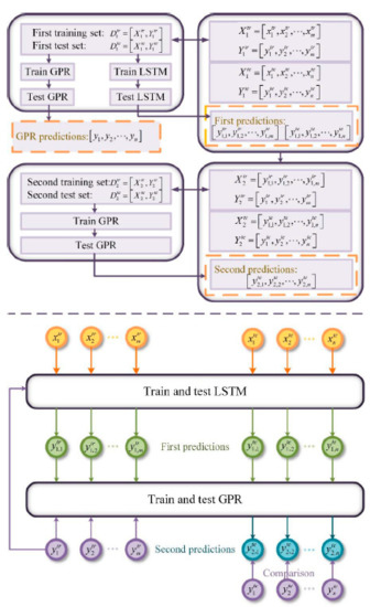
Figure 2.
Prediction flowchart of long short-term memory and LSTM and Gaussian process regression (LSTM-GPR).
3. Modeling Based on LSTM-GPR
3.1. Feature Selection Based on Weather Variables Correlation
Weather attributes employed in this paper have been summarized in Table 1. Their selection for model input completely relies on the information availability and degree of correlation with target output. Consequently, the correlation coefficient of all the eight weather parameters with solar power output is first measured and depicted in Figure 3. It follows from this figure that both visibility and temperature are mildly positively correlated with solar power, while cloud coverage and humidity are mildly negatively correlated with solar power. Additionally, other weather variables with relatively weaker correlation, including dew point, wind speed, pressure, and altimeter, should not be neglected. Only several major influencing factors are considered in most of the existing SPF methods. However, it is unreasonable to only incorporate the most important weather variables into the model input since various environmental conditions have caused different degrees of impact on solar power generation. Therefore, benefiting from the high-dimensional weather data, performance improvement can be achieved despite the higher training time cost, which can be ignored because of the offline training and speedy prediction.

Table 1.
A summary of selected weather attributes.
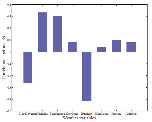
Figure 3.
Correlation coefficient of weather attributes with solar power output.
3.2. Feature Selection Based on Time Correlation
The previous section has revealed that a meaningful attempt is to comprehensively use weather information and time element for SPF. Because of the earth’s rotation, solar power generation at a specific hour of a day shows considerable time correlation, i.e., daily regularity. To intuitively display this feature, representing the four seasons in 2017, data from 10 January to 20 January, from 10 May to 20 May, from 10 July to 20 July, and from 10 October to 20 October are selected to depict the distribution of daily solar power generation, which is shown in Figure 4. Only during the period from 6:00 am to 5:00 pm is the sunshine duration, zero observations of nightly energy are negligible here. It is observed that the power output exhibits similar behavior among the days (uniform variance trend), while it exhibits diverse and irregular behavior under the terrible or rapidly variational weather conditions (abrupt turning points occurring at the hour other than 12:00 am). In regular cases, solar power generates from the beginning of a day, and then gradually increases until it peaks at noon (12:00 am), finally declines to zero as evening approaches, which distinctly implies that the solar power output is considerably pertinent to the hour of the day. To numerically present the time correlation, the correlation coefficient of the time variable with solar power output is calculated as 0.1692. Due to the limited data support, not only daily regularity but similar monthly and even annual behavior can be found and discussed.
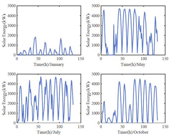
Figure 4.
Distribution of selected daily solar power generation.
3.3. LSTM-GPR Based Forecasting Modeling
Based on the above-mentioned analysis of weather and time correlation, the structure of LSTM-GPR has been defined. Eight weather attributes at a given hour and the corresponding hour of the day are thus used as the model input feature vector , solar power output at the corresponding time is directly treated as the output . Benefiting from this designed structure, short-term SPF can be achieved by using the predicted weather information. The following is to implement the hybrid model algorithm (Section 2.3) according to the defined structure. Hence, in the hybrid model, input variables of LSTM are composed of eight weather attributes and the time variable, corresponding solar power output is the output. Therefore, the first results and obtained by LSTM are the solar power output predictions. Then and are treated as the input and output to train GPR, respectively. The second predictions can be obtained according to the corresponding input in GPR.
The advancement of the introduced LSTM and the superiority of the proposed LSTM-GPR are confirmed by the comparison with other algorithms, including BPNN, individual LSTM, and GPR. It is worth noting that the same input-output structure as the hybrid model is implemented in BPNN and individual LSTM and GPR, while GPR of the hybrid model executes the second prediction between the first results forecasted by LSTM and observations.
4. Experimental Results and Discussion
4.1. Experimental Data
The solar power output and the corresponding eight weather parameters dataset of the campus of the University of Illinois in Urbana-Champaign, from 1 February 2016 to 28 October 2017, is gathered from a publicly available database [33], which has been pre-processed to obtain a consistent hourly resolution. It can be observed that sunshine duration is only during the period from 6:00 am to 5:00 pm. Hence, observations ranging from 6:00 a.m. to 5:00 p.m. are selected to implement the experiments and avoid the model performance degradation caused by the increasing variance noise from the nightly zero observed energy. Two cases with different sample sizes are used to validate the proposed hybrid model’s ability to perform highly precise point prediction and reliable interval forecasting. Detailed sample information is presented in Table 2 and elaborated on in the following chapter. All the models covered in this paper are programmed on MATLAB 2020a.
Table 2.
Sample information of two cases.
Before these raw data are fed into the model training and test, min-max normalization is used to scale the experimental data to [0,1] to degrade the negative influence resulting from the large difference in data scale.
4.2. Model Assessment Criteria
4.2.1. Assessment Criteria of Point Prediction
To qualitatively assess the models’ ability to perform SPF, commonly used assessment criteria, including Root Mean Squared Error (RMSE), Mean Absolute Error (MAE), and Mean Absolute Percentage Error (MAPE), are calculated by the SPF results and observations . The official function is written as follows. represents the number of test set samples.
4.2.2. Assessment Criteria of Interval Forecasting
(1) Coverage rate (CR)
CR [34] is defined as the ratio of the number of observation values within the prediction interval to all the observations, which is given by Equation (22). and are denoted as the number of the former and latter observations, respectively.
(2) Mean interval width (MIW)
CR can be used to assess the interval prediction performance to some extent. However, a sufficient wide interval signifies the coverage of 100%, which breaks the meaning of evaluation value and brings about heavy burden for smart grid. MIW is defined as the mean width of the prediction interval. It is obvious that a lower MIW and a higher CR suggest a more reliable prediction interval. Therefore, MC defined as the ratio of MIW to CR is introduced, which is expected to be a litter smaller.
where and are defined as the upper bound and lower bound of predictions, respectively.
4.3. Experimental Results
Three tasks require to be completed in this chapter. First is to verify the advancement of the introduced LSTM. Second, the proposed LSTM-GPR is compared with individual models in terms of point and interval prediction. Third is to confirm the efficiency and reliability of the hybrid model.
Two cases with different samples are used to test and validate the prediction performance of the proposed models. In the first experiment, the data covering 5160 samples are employed, and the last two days are selected as the forecasting days to test the performance, while the second experiment is performed with fewer samples. To ensure a fair comparison, all the involved models are trained with the same dataset and tested on the same forecasting days. The point prediction can be obtained by all the involved models, while the prediction interval can only be achieved using LSTM-GPR and individual GPR.
(1) Analysis of point prediction
The point prediction accuracy of LSTM-GPR is discussed in detail here. Numerical assessment of all the involved models has been calculated in Table 3 and intuitively depicted in Figure 5. It can be seen that LSTM produces considerable point prediction results against BPNN whenever RMSE, MAE, and MAPE are considered in the two cases, implying that LSTM taking into account the correlation between the solar power data shows strong superiority over the conventional BPNN. Thus the advancement of the introduced LSTM algorithm has been verified. For the hybrid model, we have achieved the goal of satisfactory point prediction due to the reservation of LSTM and we even obtained the results with a slight improvement. The reason is that the second training of GPR between the first predictions obtained by LSTM and observations improved the prediction performance. On the contrary, the individual GPR developed with weather and time variables exhibits disappointing performance in both cases and even worse than BPNN. Therefore, the excellent point prediction performance is mostly attributed to the LSTM application. To vividly compare the prediction accuracy, the forecasting results of all the involved models of the two cases are drawn in Figure 6 and Figure 7. The conclusion drawn from the figures is consistent with the above discovery. Consequently, the comprehensively best point prediction performance is obtained by LSTM-GPR among all the models.
Table 3.
Numerical assessment of all the involved models.
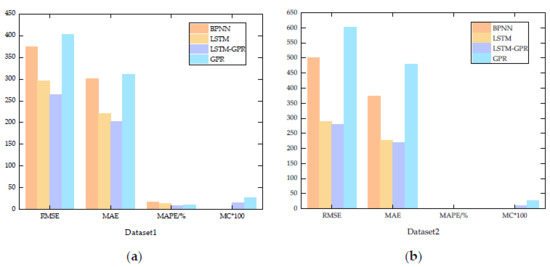
Figure 5.
Assessment criteria. (a) Assessment criteria of Dataset1, (b) Assessment criteria of Dataset2.
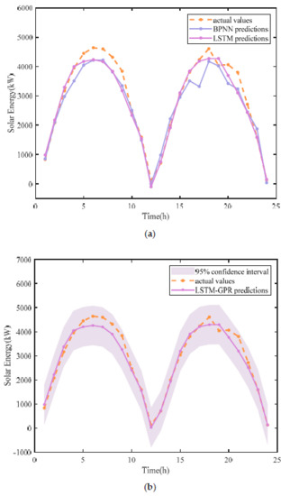
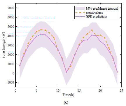
Figure 6.
Forecasting results of Datasert1. (a) Forecasting results obtained by individual LSTM and BPNN, (b) forecasting results obtained by LSTM-GPR, (c) forecasting results obtained by individual GPR.
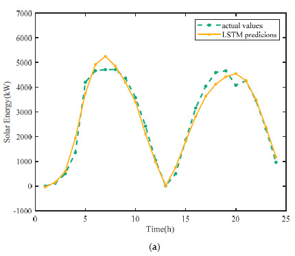
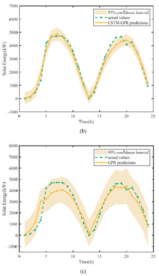
Figure 7.
Forecasting results of Datasert2. (a) Forecasting results obtained by individual LSTM and BPNN, (b) forecasting results obtained by LSTM-GPR, (c) forecasting results obtained by individual GPR.
(2) Analysis of interval forecasting
Interval forecasting reliability of LSTM-GPR is demonstrated here. Confidence coefficient is set to 95% in this work. Numerical assessment can be seen in Table 3, and the intuitive prediction interval of the two cases is drawn in Figure 6 and Figure 7. In Dataset1, benefiting from the highly accurate point prediction due to the LSTM application and second prediction of GPR, MIW obtained by LSTM-GPR is significantly smaller than that obtained by individual GPR, although both models have 100% CR. A similar phenomenon about MIW can be found in Dataset2. However, individual GPR has a little higher CR than LSTM-GPR, it is difficult to determine which model obtains a more reliable prediction interval. MC is introduced to deal with this difficulty. It is observed from Table 3 that MC of individual GPR is nearly twice as large as LSTM-GPR, which implies that the individual GPR increases CR by expanding the interval width. Hence, the prediction interval obtained by GPR has of no practical application value, and the comprehensively reliable interval forecasting performance is obtained by LSTM-GPR.
In addition, it can be found that the prediction interval is relatively wider at the volatility of solar power. Furthermore, LSTM-GPR fails in timely tracking the variability of solar power, which may be solved by constructing the complex kernel function of GPR.
According to the above comparisons and analysis, forecasting results confirm the advancement and superiority of LSTM over the conventional neural networks and demonstrate that LSTM-GPR achieves the best point prediction and interval forecasting performance.
4.4. Discussion
Based on the introduction of advanced LSTM, a novel combination strategy of LSTM and GPR is proposed to achieve a highly precise point prediction and reliable interval forecasting simultaneously for short-term SPF. However, some discussions require to be conducted here to guide the direction of future research.
(1) Due to the limited data support, time-based regularity and periodicity of solar power cannot be found by similar monthly and even annual behaviors. Therefore, a combination of month, day of the month, hour of the day, and weather parameters can be fed into the model input to improve the model structure if abundant data are available.
(2) The proposed hybrid model produces considerable results in regular cases, but it cannot track the abrupt fluctuation of solar power due to the weather disturbances, which probably partially results from the simple kernel function used in GRP. Future work will focus on the complex kernel functions adapted to the solar power data.
(3) It is worth noting that LSTM-GPR not only can be applied in SPF applications but in applications related to time series, such as wind speed and solar irradiance. In addition, SPF with high precision is directly beneficial to the combination prediction of solar power, wind power, and load in the complementary system.
(4) Environmental regulation will have consequential effects on current research. Change of requirements prescribed by environmental regulation will increase the complexity of the use of solar power. Continuing experiments on current research is necessary for the change of environmental requirements in the future.
5. Conclusions
Short-term SPF method is first developed with time element and weather attributes in this study. Additionally, LSTM is considered an attractive technique for short-term SPF and introduced. However, it fails in predicting the uncertainty range of solar power, which can be achieved by the probability prediction model, GPR. A novel hybrid model reserving LSTM’s superiority of arbitrary-length sequence dependence and exploiting GPR’s ability to predict uncertainty range is proposed. The novelty of this work lies in that deep learning technology and probability prediction methods are combined to compensate for the deficiencies of individual models and preserve their advantages. Two cases with different samples have been carried out to test and validate the performance of the proposed method. Several performance indicators have been proposed and defined for the assessment of point prediction and interval forecasting. Numeric assessment and intuitive forecasting figures have verified the advancement and superiority of LSTM by comparison with conventional BPNN. Furthermore, LSTM-GPR obtains comprehensively highly accurate point prediction and reliable forecasting interval due to the LSTM application and second prediction of GPR. Although the highly precise point prediction has been achieved, LSTM-GPR fails in timely tracking the violent fluctuation of solar power, which is the research direction for future work. In general, LSTM-GPR will become a promising technology for future SPF applications and other applications, such as load and solar irradiance prediction.
Author Contributions
Y.W. and Q.-S.H. conceived the main idea and wrote the manuscript. B.F. did the simulations. L.S. reviewed the paper and gave improvement suggestions. All authors have read and agreed to the published version of the manuscript.
Funding
This research was funded by National Key Research and Development Program under Grant 2018YFB1502900.
Institutional Review Board Statement
The study was conducted according to the guidelines of the Declaration of Helsinki, and approved by the Institutional Review Board of NAME OF INSTITUTE.
Informed Consent Statement
Informed consent was obtained from all subjects involved in the study.
Conflicts of Interest
The authors declare no conflict of interest.
References
- Wang, F.; Zhen, Z.; Liu, C.; Mi, Z.; Hodge, B.-M.; Shafifie-khah, M.; Catalão, J.P. Image phase shift invariance based cloud motion displacement vector calculation method for ultra short-term solar PV power forecasting. Energy Convers. Manag. 2018, 157, 123–135. [Google Scholar] [CrossRef]
- Masa-Bote, D.; Castillo-Cagigal, M.; Matallanas, E.; Caamaño-Martín, E.; Gutiérrez, A.; Monasterio-Huelín, F.; Jiménez-Leube, J. Improving photovoltaics grid integration through short time forecasting and self-consumption. Appl. Energy 2014, 125, 103–113. [Google Scholar] [CrossRef]
- Sun, L.; Xue, W.; Li, D.; Zhu, H.; Su, Z.-G. Quantitative Tuning of Active Disturbance Rejection Controller for FOPDT Model with Application to Power Plant Control. IEEE Trans. Ind. Electron. 2021, 1. [Google Scholar] [CrossRef]
- Wang, F.; Xiang, B.; Li, K.; Ge, X.; Lu, H.; Lai, J.; Dehghanian, P. Smart Households’ Aggregated Capacity Forecasting for Load Aggregators Under Incentive-Based Demand Response Programs. IEEE Trans. Ind. Appl. 2020. [Google Scholar] [CrossRef]
- Ismail, A.M.; Ramirez-Iniguez, R.; Asif, M.; Munir, A.B.; Muhammad-Sukki, F. Progress of solar photovoltaic in ASEAN countries: A review. Renew. Sustain. Energy Rev. 2015, 48, 399–412. [Google Scholar] [CrossRef]
- Sun., L.; Jin, Y.; Shen, J.; You, F. Sustainable Residential Micro-Cogeneration System Based on a Fuel Cell Using Dynamic Programming-Based Economic Day-Ahead Scheduling. ACS Sustain. Chem. Eng. 2021. [Google Scholar] [CrossRef]
- Van Haaren, R.; Morjaria, M.; Fthenakis, V. An energy storage algorithm for ramp rate control of utility scale PV (photovoltaics) plants. Energy 2015, 91, 894–902. [Google Scholar] [CrossRef]
- Wang, F.; Xuan, Z.; Zhen, Z.; Li, K.; Wang, T.; Shi, M. A day-ahead PV power forecasting method based on LSTM-RNN model and time correlation modification under partial daily pattern prediction framework. Energy Convers. Manag. 2020, 212, 112766. [Google Scholar] [CrossRef]
- Alonso-Montesinos, J.; Monterreal, R.; Fernández-Reche, J.; Ballestrín, J.; Carra, E.; Polo, J.; Barbero, J.; Batlles, F.; López, G.; Enrique, R.; et al. Intra-hour energy potential forecasting in a central solar power plant receiver combining Meteosat images and atmospheric extinction. Energy 2019, 188, 116034. [Google Scholar] [CrossRef]
- Ohtake, H.; Uno, F.; Oozeki, T.; Yamada, Y. The Latest Update of JMA Numerical Weather Prediction Models and its Solar Power Forecasting Errors. IEEJ Trans. Power Energy 2018, 138, 881–892. [Google Scholar] [CrossRef]
- Qing, X.; Niu, Y. Hourly day-ahead solar irradiance prediction using weather forecasts by LSTM. Energy 2018. [Google Scholar] [CrossRef]
- Pattanaik, D.; Mishra, S.; Khuntia, G.P.; Dash, R.; Swain, S.C. An innovative learning approach for solar power forecasting using genetic algorithm and artificial neural network. Open Eng. 2020, 10, 630–641. [Google Scholar] [CrossRef]
- Lin, K.-P.; Pai, P.-F. Solar power output forecasting using evolutionary seasonal decomposition least-square support vector regression. J. Clean. Prod. 2016, 134, 456–462. [Google Scholar] [CrossRef]
- Wang, H.; Lei, Z.; Zhang, X.; Zhou, B.; Peng, J. A review of deep learning for renewable energy forecasting. Energy Convers. Manag. 2019, 198, 111799. [Google Scholar] [CrossRef]
- Sherstinsky, A. Fundamentals of Recurrent Neural Network (RNN) and Long Short-Term Memory (LSTM) Network. Phys. D Nonlinear Phenom. 2020, 404, 132306. [Google Scholar] [CrossRef]
- Li, G.; Wang, H.; Zhang, S.; Xin, J.; Liu, H. Recurrent Neural Networks Based Photovoltaic Power Forecasting Approach. Energies 2019, 12, 2538. [Google Scholar] [CrossRef]
- Zhou, H.; Zhang, Y.; Yang, L.; Liu, Q.; Yan, K.; Du, Y. Short-term Photovoltaic Power Forecasting based on Long Short Term Memory Neural Network and Attention Mechanism. IEEE Access 2019, 7, 78063–78074. [Google Scholar] [CrossRef]
- Lee, W.; Kim, K.; Park, J.; Kim, J.; Kim, Y. Forecasting Solar Power Using Long-Short Term Memory and Convolutional Neural Networks. IEEE Access 2018, 6, 73068–73080. [Google Scholar] [CrossRef]
- Mitsuru, K.; Yusuke, E.; Hiromasa, S.; Ikeda, R.; Kusaka, H. Probabilistic Solar Irradiance Forecasting by Conditioning Joint Probability Method and its Application to Electric Power Trading. IEEE Trans. Sustain. Energy 2018, 10, 983–993. [Google Scholar]
- Wen, Y.; Alhakeem, D.; Mandal, P.; Chakraborty, S.; Wu, Y.-K.; Senjyu, T.; Paudyal, S.; Tseng, T.-L. Performance Evaluation of Probabilistic Methods Based on Bootstrap and Quantile Regression to Quantify PV Power Point Forecast Uncertainty. IEEE Trans. Neural Netw. Learn. Syst. 2020, 31, 1134–1144. [Google Scholar] [CrossRef]
- Sheng, H.; Xiao, J.; Wang, P. Lithium Iron Phosphate Battery Electric Vehicle State of Charge Estimation based on Evolutionary Mixture Gaussian Regression. IEEE Trans. Ind. Electron. 2016, 64, 544–551. [Google Scholar] [CrossRef]
- Samuelsson, O.; Björk, A.; Zambrano, J.; Carlsson, B. Gaussian process regression for monitoring and fault detection of wastewater treatment processes. Water Sci. Technol. 2017, 75, 2952. [Google Scholar] [CrossRef]
- Kushwaha, V.; Pindoriya, N.M. A SARIMA-RVFL hybrid model assisted by wavelet decomposition for very short-term solar PV power generation forecast. Renew. Energy 2019, 140, 124–139. [Google Scholar] [CrossRef]
- Rana, M.; Koprinska, I.; Agelidis, V.G. Univariate and multivariate methods for very short-term solar photovoltaic power forecasting. Energy Convers. Manag. 2016, 121, 380–390. [Google Scholar] [CrossRef]
- Bouzerdoum, M.; Mellit, A.; Pavan, A.M. A hybrid model (SARIMA–SVM) for short-term power forecasting of a small-scale grid-connected photovoltaic plant. Sol. Energy 2013, 98, 226–235. [Google Scholar] [CrossRef]
- Kim, J.G.; Kim, D.H.; Yoo, W.S.; Lee, J.; Kim, Y.B. Daily prediction of solar power generation based on weather forecast information in Korea. IET Renew. Power Gener. 2017, 11, 1268–1273. [Google Scholar] [CrossRef]
- Lu, H.J.; Chang, G.W. A Hybrid Approach for Day-Ahead Forecast of PV Power Generation. IFAC-PapersOnLine 2018, 51, 634–638. [Google Scholar] [CrossRef]
- Wessam, E.B.; Peter, T.; Ulrich, W. Day-ahead probabilistic PV generation forecast for buildings energy management systems. Sol. Energy 2018, 171, 478–490. [Google Scholar]
- Sun, G.; Jiang, C.; Wang, X.; Yang, X. Short-term building load forecast based on a data-mining feature selection and LSTM-RNN method. IEEJ Trans. Electr. Electron. Eng. 2020, 15, 1002–1010. [Google Scholar] [CrossRef]
- Fischer, T.; Krauss, C. Deep learning with long short-term memory networks for financial market predictions. Eur. J. Oper. Res. 2017, 270, 654–669. [Google Scholar] [CrossRef]
- Tolba, H.; Dkhili, N.; Nou, J.; Eynard, J.; Thil, S.; Grieu, S. GHI forecasting using Gaussian process regression: Kernel study. IFAC-PapersOnLine 2019, 52, 455–460. [Google Scholar] [CrossRef]
- Wojtkiewicz, J.; Hosseini, M.; Gottumukkala, R.; Chambers, T.L. Hour-Ahead Solar Irradiance Forecasting Using Multivariate Gated Recurrent Units. Energies 2019, 12, 4055. [Google Scholar] [CrossRef]
- Kuzmiakova, A.; Colas, G.; McKeehan, A. Machine Learning for Solar Energy Prediction. Available online: https://github.com/ColasGael/Machine-Learning-for-Solar-Energy-Prediction (accessed on 1 July 2020).
- Ranran, L.; Yu, J. A wind speed interval prediction system based on multi-objective optimization for machine learning method. Appl. Energy 2018, 228, 2207–2220. [Google Scholar]
Publisher’s Note: MDPI stays neutral with regard to jurisdictional claims in published maps and institutional affiliations. |
© 2021 by the authors. Licensee MDPI, Basel, Switzerland. This article is an open access article distributed under the terms and conditions of the Creative Commons Attribution (CC BY) license (http://creativecommons.org/licenses/by/4.0/).