Article

Total Investment in Fixed Assets and the Later Stage of Urbanization: A Case Study of Shanghai

1
School of Architecture and Urban Planning, Guangdong University of Technology, Guangzhou 510006, China
2
Media Lab, Massachusetts Institute of Technology, Cambridge, MA 02139, USA
3
School of Architecture and Urban Planning, Tongji University, Shanghai 200092, China
4
Institute of Urban and Demographic Studies, Shanghai Academy of Social Sciences, Shanghai 200020, China
5
School of Civil Engineering and Architecture, Zhejiang University of Science and Technology, Hangzhou 310023, China
6
School of Automation, Guangdong University of Technology, Guangzhou 510006, China
*
Authors to whom correspondence should be addressed.
Sustainability 2021, 13(7), 3661; https://doi.org/10.3390/su13073661
Submission received: 20 February 2021 / Revised: 18 March 2021 / Accepted: 21 March 2021 / Published: 25 March 2021

Abstract

:
After more than 40 years’ opening-up and reform, China’s urbanization has entered a new type of urbanization. In order to reveal the rule of different infrastructure investments and urbanization relationships, this paper uses Shanghai as a case by applying econometric methods to study the detailed relationship between different indicators from 1990 to 2019. Firstly, we quantify that each variable has a long-term co-integration relationship with urbanization by co-integration test. And we found that the real estate is a main driving force of urbanization while the construction project investment plays an important role in promoting the urbanization rate in the studied period. Secondly, according to the Granger test, our study illustrates that each variable has a bilateral Granger relationship with urbanization while the urbanization rate has more Granger causality impact on the studied variables. Thirdly, based on impulse response test and variance decomposition analysis, we found that urbanization rate with other variables accounts for the majority of the percentage of impacts while the total investment in fixed assets and its three categories contribute a small amount to the urbanization rate. Finally, we propose policy suggestions to strengthen healthy urbanization development in Shanghai.

1. Introduction

Urbanization research has been a global issue since the first industrial revolution. Urbanization is the result of, for example, the social production reform of the human production method, the way of life, and residential type, and a natural, historical urban social evolutional process of the population centralization and intensification from rural areas to urban areas [1], Urbanization is necessary for social progress and considered an engine of modernization and economic growth [2]. China is undergoing unprecedented urbanization, which we propose is the greatest human-resettlement experiment in world history.
The urbanization of countries or regions differs in, for example, starting period, development speed, and current urbanization rate. However, Ray M. Northam (1979) pointed out that global urbanization can be summarized as an “S” curve [3]. Furthermore, the urbanization rate curve can be divided into two main stages—early and later—according to the acceleration of the urbanization rate growth. Notably, in Figure 1, point A in the urbanization rate curve is an inflection of two stages. In the early stage, the curve is no more than the inflection point and the curve is characterized by acceleration; thus, it can be classified into the starting period and acceleration period. In the later stage, the curve is more than the inflection point and changes from an accelerating state to a decelerating state or stationary state, and it can be divided into a deceleration period and stationary period.
Chinese cities’ urbanization has distinct characteristics. Specifically, after China’s opening-up and reform, especially after the 1998 real estate reform, a population shift occurred from rural to urban areas. However, with the development of urbanization, China’s economy has a new normal, and its economic growth rate has shifted from high to medium; therefore, China is promoting a “new type of people-centered urbanization” policy to continue the current economic situation [4].
Shanghai is the biggest city in China. Its urbanization rate increased from 58.7% in 1978 to 90.4% in 2019, and after the policy of 1990 Pudong District development was implemented, the Shanghai urban population increased from 13.34 million (1990) to 24.28 million (2019). As is shown in Figure 1, Shanghai’s current urbanization state is in a stationary period of the later stage of urbanization.
The growth in the urban population caused substantial demand for basic needs, for example, urban infrastructure for daily life including residential buildings; therefore, the Shanghai government had to use the total investment in fixed assets (i.e., construction project investment, real estate investment, farmers’ investment) every year to fulfill the needs resulting from urbanization. In this paper, the total investment in fixed assets is considered an urban infrastructure investment, which is the foundation of a city or, as one historian proposed, “technological sinews” built to fulfill the needs of society [5]. The total investment in fixed assets is the amount of work involved in the construction and purchase of fixed assets in monetary terms and a comprehensive index reflecting the investment scale, speed, proportional relationship, and utilization direction.
Thus, in this context, we aim to determine the influencing mechanism between urbanization and the total investment in fixed assets, which is dominated by the government.
Studies had attempted to explain the mechanism of the urbanization process [2] and the infrastructure investment [6]. For example, Tian et al. (2017) examined the driving forces of Shanghai land use change from the perspectives of state-led growth and bottom-up development by analyzing Landsat Thematic Mapper(TM) images and land use maps; they concluded that state-led growth played an important role in the non-agricultural land expansion and that urban planning played a main role in regulating the space to accommodate the migratory population and economic growth [7].
Maparu et al. (2017) studied different sub-sectors of transport infrastructure to find its long-run relationship and direction of causality with economic development and urbanization. Their results indicated existence of long-run relationship between transport infrastructure and economic development [8].
Grafe and Mieg (2019) discussed a conceptual model for critically engaging with the effects of financialization on contemporary cities. It concluded by outlining some of the spatial effects of the UK’s changing financial ecology of urban infrastructure [9].
Shannon et al. (2018) contributed to debates on urban land governance and sustainable urban development in Africa by providing an empirical analysis of forced displacement and resettlement associated with infrastructure development in Beira city, Mozambique. They concluded by arguing that forced displacement and resettlement should be understood as a deliberate and systematic feature of urban infrastructure development, through which new social-spatial arrangements are created [10].
The literature has also studied the overinvestment problem in China, for example, Tang et al. (2017) found that China’s economy is a strong investment driver [11]. Guo and Shi (2018) studied high investment in public infrastructure in China and found that public infrastructure investment increases when local governments capture returns from investment in land improvement [12].
However, few studies have investigated the detailed relationship between urbanization and the total investment in fixed assets. Notably, the studies of construction project investment, real estate investment, and farmers’ investment have received little attention in the literature, and these are the composition of the total investment in fixed assets. Therefore, this study attempts to fill the gap in the literature by exploring the relationship between these three factors and urbanization in the context of Shanghai as a case study.
The second contribution of this paper is its use of the generalized impulse response to trace the effect of a shock on current and future values of endogenous variables and to compare the influencing magnitude between indicators. We conduct this investigation by applying the variance decomposition technique.

2. Literature Review

An extensive literature has explored the relationship between urbanization and various aspects, for example, urbanization and economic growth, and urbanization and infrastructure investment, in the context of developing and developed countries by using different methodologies.
Traditionally, China’s land-centered urbanization is a type of “low-quality urbanization” characterized by high investment and expansion and a low level of quality and sustainability [2].
The research on the relationship between urbanization and economic aspects is diverse. Some researchers have proposed that urbanization has substantially promoted economic development in the past few decades [13] and that regional economic integration can improve urbanization efficiency [14]. Other researchers have focused on foreign direct investment (FDI), to reveal the relationship between FDI and urbanization. For example, Wu and Heerink (2016) found that the FDI growth rate has a positive and significant impact on the growth rate of illegal land use when there is a high degree of fiscal decentralization [15], and Vongpraseuth and Choi (2015) [16], Lin and Benjamin (2018) [17] have conducted similar research. By contrast, one study found that FDI has a limited role in urban investment [18].
Regarding the relationship between urbanization and infrastructure investment, the conclusions in the literature are diverse, and the relationship is unclear. Some studies have found that higher infrastructure investment may lead to a higher urbanization rate, and most of the literature has focused on various infrastructure investments and urbanization rate. More specifically, four strands of literature are related to infrastructure investment and urbanization.
The first strand of the literature has focused mainly on the real estate or housing market. Generally, urban land expansion is affected by the market forces [19], especially the real estate or housing market. Cao et al. (2018) found that the real estate market is the major source of urban infrastructure construction funding and a main driving force of urbanization [20]. However, the real estate market may negatively influence urban sustainable development [21], especially the economic “bubble” that burst in the construction sector [22].
The second strand of the literature has focused on the relationship between urbanization and specific urban infrastructure, for example, transport infrastructure [8,23,24,25], water infrastructure [26], or spatial infrastructure distribution [27]. Most of this research has attempted to examine the roles of different infrastructure investments in promoting economic development, environmental change, urbanization, or quality of life for residents. For example, Chen et al. (2016) investigated the impact of high-speed rail investment on the economy and environment in China by using a computable general equilibrium model [24]; their results suggest that rail investment in China over the past decade has been a positive stimulus to the economy and that the economic impacts of rail investment are achieved primarily through induced demand and output expansion; by contrast, the contribution from a reduction of rail transportation costs and rail productivity increases were modest. Kim and Yook (2018) analyzed how the benefit assessment of roadway investment projects changes when Value of Time (VOT) is applied according to trip length and found that applying the differentiated VOT by trip length tends to increase the benefit [23].
The third strand of the literature has investigated the topic of urbanization from multiple perspectives, for example, from five aspects including population, resources, environment, development and satisfaction [28], four aspects including economic growth, energy consumption and financial development [29], three aspects including urbanization, human capital and ecological footprints [30], three aspects including settlements isolation, land use changes and poverty [31], three aspects including economic growth, urbanization and air pollutants [32], and three aspects including population inflow, social infrastructure and urban vitality [33].
The fourth strand of the literature has been related to mainly sustainable urbanization or green investment [34]. For example, Kennedy et al. (2016) discussed China’s urbanization, climate change, and interactions between infrastructure sectors, and the transformation of its industry [34]. The solutions that have been proposed are, for example, green investment [34], sustainable urban infrastructure [35], urban green infrastructure (UGI) planning [36], and low-carbon growth strategies or planning for China’s development. For example, Davies and Lafortezza (2017) found that UGI planning principles and related concepts are present to some degree in strategic greenspace planning in Europe and suggest that enhancing network connectivity is key to the development of UGI [36].
The literature on scales can be divided into four categories: national scale [37], province scale [38], city scale [7], and regional scale [19].
Additionally, many studies have focused on urban and rural areas because a higher urbanization rate may cause social problems such as gentrification [39], spatial inequality [40], and differentiation between urban and rural areas [41]. For example, Gao et al. (2020) focused on Shanghai rural–urban land transition and found that the material stocks from residential buildings in Shanghai increased 41-fold from 1950 to 2010 and that the material stocks experienced asynchronized growth in rural areas, central urban areas, and rural–urban land transition zones (RULT zones) [42].
Moreover, some literature has investigated social problems caused by the related infrastructure investment. For example, Wesołowska (2016) illustrated that the location and construction process of new public investments of urban infrastructure, technical and social, lead to numerous protests held by local communities [43]. Huang and Wei (2016) found that the spatial inequality of FDI can intensify uneven economic development. Agglomeration effects have replaced institutional factors to become one of the most significant factors influencing the FDI inequality among cities [40].
Although some of the literature has attempted to examine the relationship between infrastructure investment and urbanization, most have focused on environmental or economic impacts but not the detailed relationship between infrastructure investment and urbanization and their impacts on urbanization processes, such as investments in construction projects, real estate, and farmers. Notably, because China’s urbanization has entered a new type of urbanization, it is important to reveal the rules of different infrastructure investments and urbanization relationships to fulfill the goal of high-quality urbanization by adjusting the infrastructure investment strategy.
Investments in construction projects, real estate, and farmers would substantially shape the space, urban or rural, contributing to the urbanization rate.
Therefore, to explore the detailed relationship between different infrastructure investments and urbanization, we use Shanghai as an example and consider different infrastructure investments, namely, total investment in fixed assets, construction project investment, real estate investment, and farmers’ investment, by using multiple econometric methods to explore, in detail, the relationship between infrastructure investment and urbanization.

3. Materials and Method

3.1. Data Source

We collected the raw data from the Shanghai Statistical Yearbook (1990–2019) [44], including total investment in fixed assets ( T I t ) and urbanization rate ( U R t ). Total investment in fixed assets can be classified into three categories: construction project investment ( C P I t ), real estate investment ( R E I t ), and farmers’ investment ( F I t ). These data are shown in Table A1 (see Appendix A).
According to the World Urbanization Prospects published by the United Nations [45], the percentage of the urban population in the total population is one of the most important indices of urbanization. The raw datasets can be extracted from the annual urban population ( U P t ) and annual total population ( P t ). The urbanization rate ( U R t ) can be defined as Equation (1).
U R t = U P t P t × 100 %
where t is the year.
In addition, to prevent the data of each time series from generating heteroscedasticity before conducting the methodology, the data are analyzed by the logarithm transformation, making it easy for the obtained data to become a stationary sequence.

3.2. Econometric Methodology

3.2.1. Unit Roots Test

In this paper, to confirm the time series are stationary, we conduct multiple unit roots tests: the augmented Dickey–Fuller (ADF) test, the Phillips–Perron (PP) test, the Dickey–Fuller test that uses a generalized least squares test (DF GLS), and the Kwiatkowski–Phillips–Schmidt–Shin (KPSS) test.
The ADF test is commonly used because it can avoid higher-order serial correlation effects and can be described as follows: considering that the time series of ( X t ) has the pth-order autoregressive process [46,47].
x t = a 0 + a 1 x t 1 + a 2 x t 2 + + a p x t p + ε t
Equation (2) can be transformed into Equation (3) by adding a time-trend term.
Δ x t = a 0 + r x t 1 + a 2 t + i = 2 p δ i Δ x t r + 1 + ε t
r   =   [ 1     i = 2 p a i ] ,   δ = j = i p a j
In the ADF test, the null hypothesis is H 0 : r = 0. If this is true, x t has no root. Dickey and Fuller (1981) found that the critical values for r = 0 depend on the form of the regression and sample size [46].
Dickey and Fuller (1979) have provided three additional F-statistics ( φ 1 , φ 2 , and φ 3 ) to test a joint hypothesis on the coefficients [47]. The null hypothesis r = a 0 = 0 is tested by using the φ 1 statistic. When a time trend is included in the regression, the joint hypothesis a 0 = r = a 2 = 0 is tested by using the φ 2 statistic, and the joint hypothesis r = a 2 = 0 is tested by using the φ 3 statistic.
However, although the ADF test has been widely used, its disadvantage is low efficacy, especially when the sample size is too small and there is high autocorrelation in the dataset. Thus, we conduct four different unit root tests to examine the variables stationarity.
Furthermore, Maddala and Kim (1999) demonstrated the problems of different unit root tests and proposed the method of ADF, DFGLS, PP, and KPSS [48].
The details of the unit tests are in the literature [48,49].

3.2.2. Johansen Co-Integration Test

The time series stability test and co-integration test are usually conducted to avoid spurious regression before the Granger causality test.
Granger causality can be implemented if the long-term co-integration relationship is significant. In this study, the Jahansen and Juselius co-integration (JJ) test is employed to investigate the co-integration relationship. The JJ test can be expressed as Equations (4) and (5):
Δ l n ( U R t ) = α 1 + i = 1 p γ 1 i Δ l n ( U R t i ) + i = 0 p α 1 i Δ l n ( T I t i ) + υ 1 l n ( U R t 1 ) + δ 1 l n ( T I t 1 ) + u t 1
Δ l n ( U R t ) = α 2 + i = 1 p γ 2 i Δ l n ( U R t i ) + i = 0 p α 2 i Δ l n ( C P I t i ) + i = 0 p α 3 i Δ l n ( R E I t i ) + i = 0 p α 4 i Δ l n ( F I t i ) + υ 2 l n ( U R t 1 ) + δ 2 l n ( C P I t 1 ) + δ 3 l n ( R E I t 1 ) + δ 4 l n ( F I t 1 ) + u t 2
where γ n i and α n i (n = 1,2,3,4) are the coefficient parameters, α n (n = 1,2) are the constant terms, Δ represents the first-order difference of the variables, p is the maximum lag period, and u n t (n = 1,2) is the stationary time series. The null hypothesis ( H n 0 : υ n = δ n = 0 ), supposing no co-integration relationship between variables, is tested against the alternative hypothesis ( H n 1 : υ n δ n 0 ) of the existence of co-integration relationships.

3.2.3. VAR Model and Granger Causality Test

After the co-integration test, we build the corresponding two vector error regression models (VARs) with CO2 emission and four other indicators, respectively. Next, the modified Granger causality test based on [50] is used to verify whether any lag value of a variable affects the current value. The specification of the Granger causality test can be described in the following forms:
The VAR 1 model describes the relationship between the U R t and T I t :
Δ l n ( U R t ) = α 1 + i = 1 d m a x α 1 i Δ l n ( U R t i ) + i = 1 d m a x β 1 i Δ l n ( T I t i ) + ε 1 t
Δ l n ( T I t ) = α 2 + i = 1 d m a x α 2 i Δ l n ( U R t i ) + i = 1 d m a x β 2 i Δ l n ( T I t i ) + ε 2 t
The VAR 2 model describes the relationship between the U R t and C P I t :
Δ l n ( U R t ) = α 3 + i = 1 d m a x α 3 i Δ l n ( U R t i ) + i = 1 d m a x β 3 i Δ l n ( C P I t i )   + i = 1 d m a x β 4 i Δ l n ( R E I t i ) + i = 1 d m a x β 5 i Δ l n ( F I t i ) + ε 3 t
Δ l n ( C P I t ) = α 4 + i = 1 d m a x α 4 i Δ l n ( U R t i ) + i = 1 d m a x β 6 i Δ l n ( C P I t i )   + i = 1 d m a x β 7 i Δ l n ( R E I t i ) + i = 1 d m a x β 8 i Δ l n ( F I t i ) + ε 4 t
where α n i and β n i (n = 1,2,3,4,5,6,7,8) are the coefficient parameters, α n (n = 1,2,3,4) is the constant term, dmax is the optimal lag period, and ε n t (n = 1,2,3,4) represents the stochastic terms for fitted models.
We applied the logarithm transformation of these time series data to prevent the data of each time series from generating heteroscedasticity, making it easy for the obtained data to become a stationary sequence. The advantage of the aforementioned Equations (4)–(9) is that they can be applied without considering the long-term co-integrated variables.

3.2.4. Impulse Response Functions and Variance Decomposition

Following the related literature, we employ impulse response analysis and variance decomposition, proposed by Sims [51], to examine how an unexpected shock in one of the variables influences the dynamic behavior of other variables and uncovers simplifying structures in a large set of variables.
In macroeconomic analysis, the term “variance decomposition” or, more precisely, “forecast error variance decomposition,” is used more narrowly for a specific tool for interpreting the relations between variables described by VAR models.
Specifically, while impulse response functions trace the effects of a shock to one endogenous variable on to the other variables in the VAR, variance decomposition separates the variation in an endogenous variable into the component shocks to the VAR. Thus, the variance decomposition provides information on the relative importance of each random innovation in affecting the variables in the VAR.

4. Empirical Results

In this section, we first analyze the descriptive statistics data to ascertain the change in the variables. Second, the variables are tested by different unit root test to ascertain the stationary series of all the variables. Third, we conduct the co-integration test to reveal whether the total investment in fixed assets related variables had a long-run relationship with urbanization rate. Finally, we use the VAR model to further analyze the Granger causality between the carbon urbanization rate and other indicators.

4.1. Descriptive Statistics Analysis

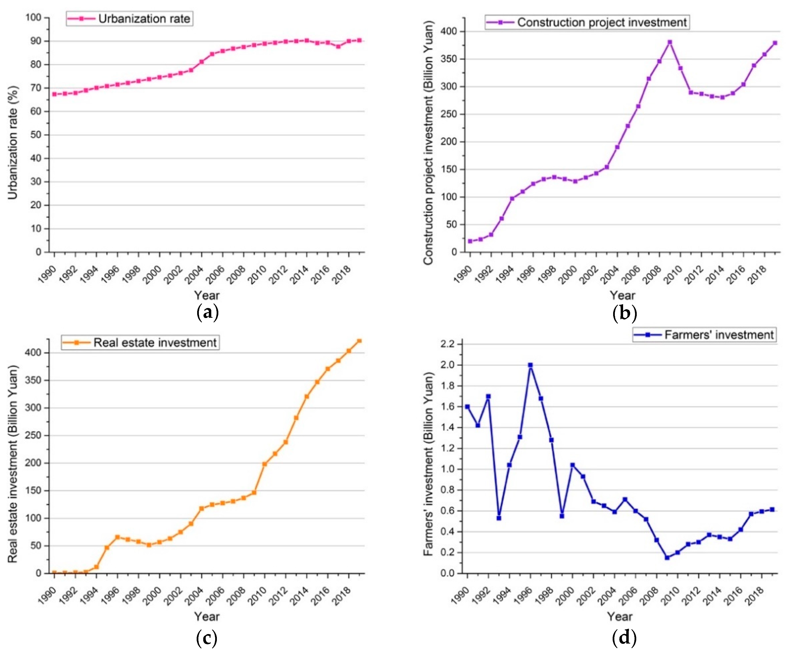
Figure 2 illustrates the temporal evolution of the variables from 1990 to 2019.
The total investment in fixed assets increased steadily from 22.71 billion yuan (in 1990) to 35.74 billion yuan (in 1992) and almost doubled to 65.39 billion yuan (in 1993) and increased to 801.98 billion yuan (in 2019), except for a small fluctuation in 1998–2001 and 2010–2012. The average growth rate of the total investment in fixed assets in each year of the studied period is 15%.
The reason for this may be twofold: the continuous growth of GDP and the considerable financial revenue in Shanghai, and policies such as the establishment of the Pudong New Area in 1993, the 1998 economic crisis the and the 2010 Shanghai World Expo. Thus, the Shanghai government has a sustained investment ability in the total investment in fixed assets, with a fluctuation of the amount due to the special events.
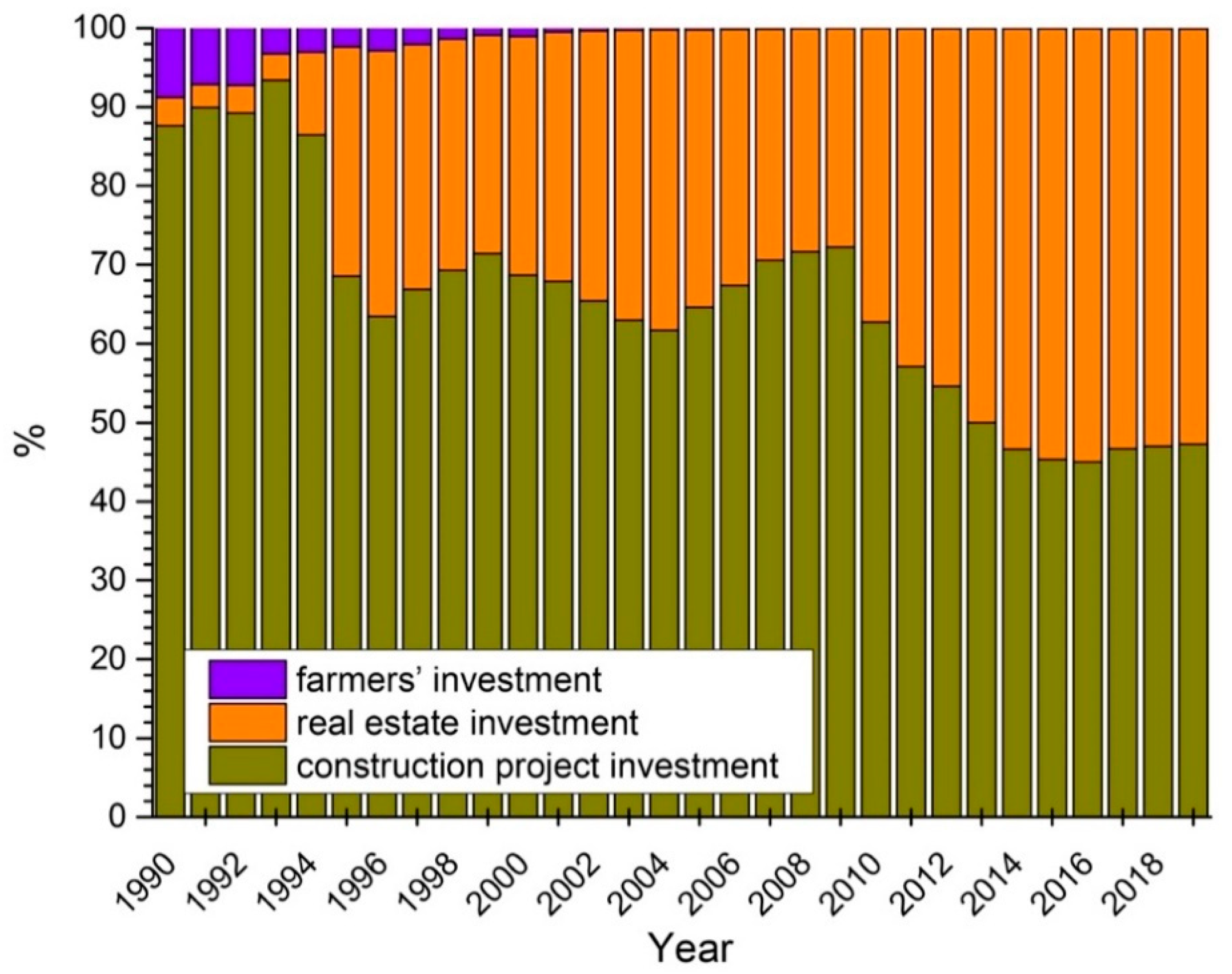
Specifically, as shown in Figure 3, the trend of construction project investment and farmers’ investment is decreasing during the studied period. The percentage of two categories decreases from 87.66% (1990) and 8.75% (1990) to 47.28% (2019) and 0.08% (2019), respectively. By contrast, the proportion of real estate investment increases from 3.59% (1990) to 52.63% (2019).
In addition, the amount of construction project investment increases from 19.91 billion yuan (1990) to the peak point of 380.76 billion yuan (2009) and finally to 379.19 billion yuan (2019). Real estate investment increases from 0.82 billion yuan (1990) to 146.42 billion yuan (2009), and it increases steadily after 2010 and then reaches 422.15 billion yuan (2019). However, farmers’ investment decreases from 1.60 billion yuan (1990) to the minimum point of 0.15 billion (2009) and finally reaches 0.61 billion yuan (2019).
Possible reasons for the aforementioned changes are Shanghai’s urban policies (i.e., 1998 real estate reform) and its special city events (i.e., 2010 Shanghai World Expo).
Moreover, the urbanization rate had a changing trend similar to other indicators between different periods. However, the urbanization rate had a fluctuation in 2014–2015 but increased again after 2015 and reached 90.4% in 2019.

4.2. Results of Stationarity Test

The time series should be a stationary sequence before this dataset is analyzed by other econometric methods [52]; moreover, the time series must be turned into the first-order differencing stationary series if the estimated parameters are biased that making it hard to give an effective explanation to the reality [53].
Furthermore, because different lag structures may have different unit root test results, we conduct our analysis by using the Akaike information criterion (AIC), which is widely used in the literature.
Table A1, Table A2, Table A3 and Table A4 (Appendix A) provide the results of four traditional unit root tests: ADF, PP, DF GLS, and KPSS. All four tests demonstrate that all the variables are non-stationary in their level data (Intercept, Intercept and trend, None), namely, I(0). However, all the variables are integrated of the first-order, namely, I(1). Therefore, we can proceed with the co-integration test.
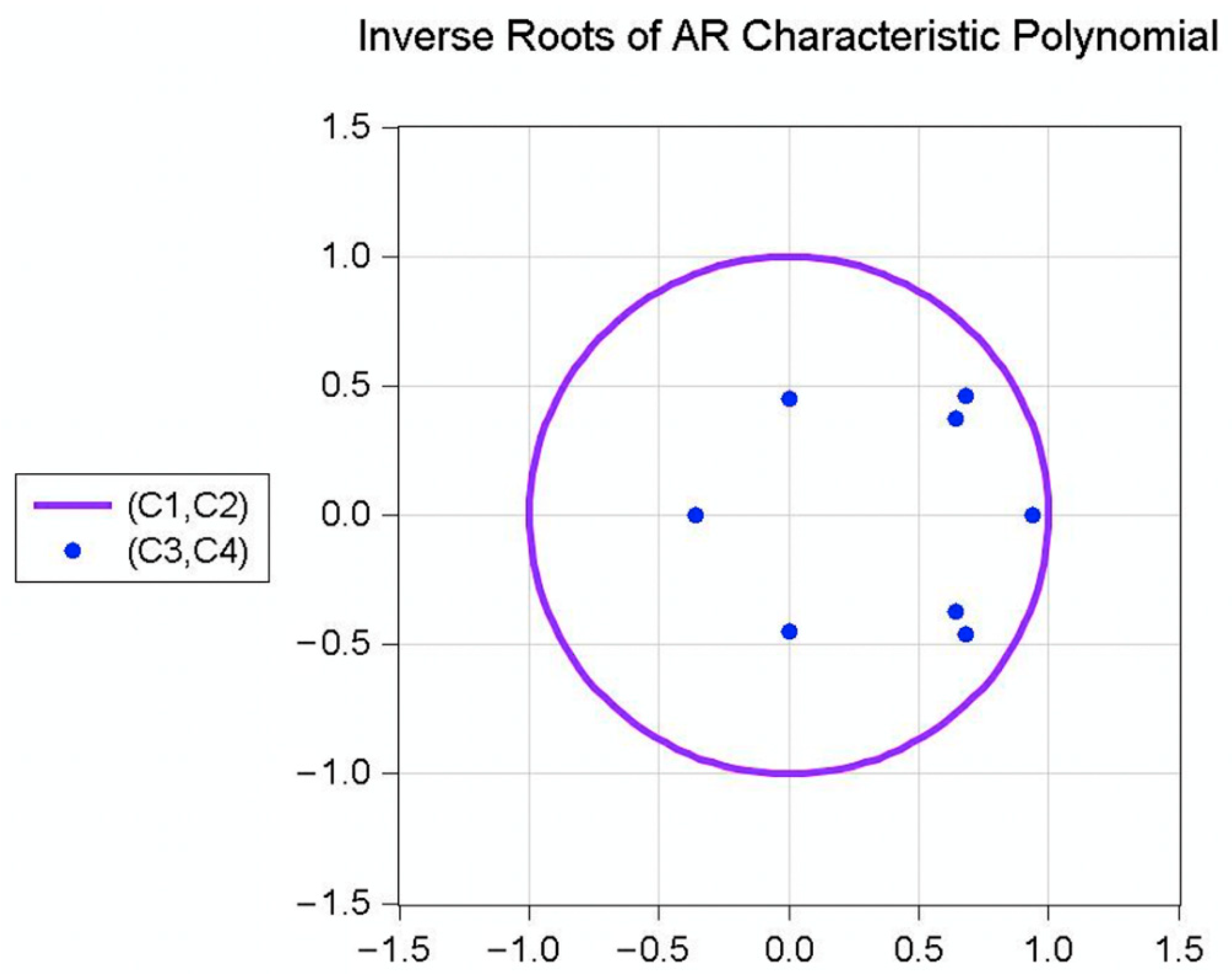
We also use the characteristic root test [54] to examine the stability of the VAR models (Appendix A Figure A1 and Figure A2), and the results show that the VAR models are stable because the characteristic roots are less than 1 or are within the unit circle. Thus, the VAR models are valid.

4.3. Results of Co-Integration Test

Next, we apply Jonhanse and Juselius co-integration test to assess if there is a long-term relationship between the selected indicators. More specifically, both the trace test and maximum eigenvalue test are used to identify co-integration relationship. The results of Jonhanse and Juselius tests are shown in Table A6.
Moreover, the Jonhanse and Juselius co-integration test configuration of the co-integration test is set up to be “no intercept or trend in test VAR,” and the lag intervals are selected to be “1 to 1”.
As shown in Table 1, the trace test and Max-eigenvalue test demonstrate that there is at least one long-run co-integrating relationship between urbanization rate and other indicators at the 0.05 level.
And on the basis of the regression results, the linear relationship between the urbanization rate and selected indicators can be transformed into Equations (10) and (11):
l n U R = 0.042437 × l n R E I + 0.253661 × l n F I + 0.479965 × l n C P I ( 0.01367 )   ( 0.00808 )   ( 0.01410 )
l n U R = 0.518738 × l n T I ( 0.01114 )
The standard errors are marked in parentheses. Equation (10) illustrates the relationship of urbanization rate ( l n U R ) and three categories of the total investment in fixed assets ( l n F I , l n C P I , and l n R E I ), and Equation (10) reveals that a positive long-run relationship between l n U R and l n F I , l n C P I , and l n R E I . Equation (11) shows the relationship of urbanization rate ( l n U R ) and the total investment in fixed assets ( l n T I ) and reveals a positive long-run relationship between l n U R and l n T I .
Furthermore, the estimated coefficients of Equations (10) and (11). can be used as the long-run elasticities to analyze the relationship between the variables. Therefore, on the basis of the aforementioned equations, we can infer that the construction project investment ( C P I t ) has a higher impact on urbanization rate than real estate investment ( R E I t ) and farmers’ investment ( F I t ). As the construction project investment ( C P I t ) increases by 1%, the urbanization rate ( U R t ) would increase by almost 0.48%, while real estate investment ( R E I t ) and farmers’ investment ( F I t ).increases by 1%, the urbanization rate would increase by 0.04% and 0.25%, respectively.
Regarding the relationship between urbanization rate ( U R t ) and total investment in fixed assets ( T I t ), we can infer from Equation (2) that when the total investment in fixed assets ( T I t ) increases by 1% investment, the urbanization rate ( U R t ) increases by almost 0.52%.

4.4. Results of Granger Causality Test

Before conducting the Granger causality test, we employ the sequential modified LR test statistic (LR), final prediction error (FPE), AIC, Schwarz information criterion (SC), and Hannan–Quinn information criterion (HQ) as the optimal lag length test types to ascertain the optimal lag length of different Granger causality tests. According to Liew [55] and Gutierrez et al. [56], AIC and FPE are superior to other criteria because they can provide considerable advantages in terms of selecting the correct VAR model, and AIC is the most preferable one in their studies. Therefore, we identify the optimal lag according to AIC, FPE, LR, SC, and HQ in sequence. Appendix A Table A5 is the optimal lag length results, which demonstrate the different optimal lag lengths of different variables’ groups by using different test methods. Next, we conduct the Granger causality test by integrating all the optimal lag lengths results.
In Table 2, the optimal lag lengths between urbanization rate and other indicators are as follows: Group ( l n U R , l n F I , l n C P I and l n R E I ) are lag 2–4, Group ( l n U R , l n T I ) are lags 2, 3, and 8.
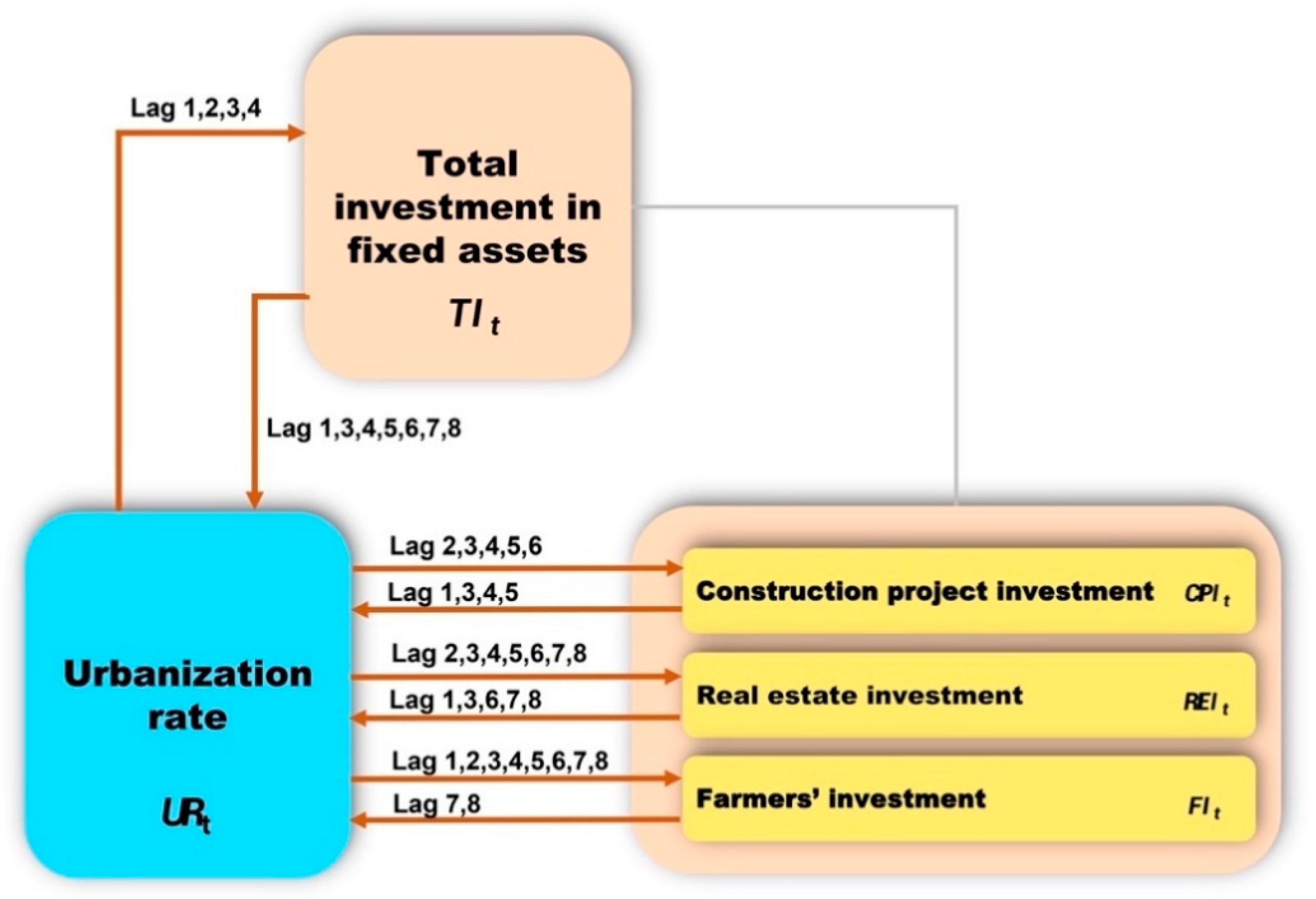
In addition, Appendix A Table A7 presents the details of the Granger causality test of urbanization and the other seven indicators. The results are summarized in Figure 4.
In Figure 4, the relationship between urbanization rate and total investment in fixed assets has a bilateral Granger causality relationship in lags 1, 3, and 4 and has a one-way Granger causality relationship in lags 2, 5, 6, 7, and 8.
Regarding the relationship between urbanization rate and the other three indicators, in different lag periods, both bilateral Granger causality relationship and one-way direction Granger causality relationship are observed. Specifically, there is a bilateral relationship in lags 3, 4, and 5 ( C P I t and U R t ); lags 6, 7, and 8 ( R E I t and U R t ); and lags 7 and 8 ( F I t and U R t ) and a one-way relationship in lags 1 and 2 ( C P I t and U R t ); lags 1, 2, 4, and 5 ( R E I t and U R t ); and lags 1, 2, 3, 4, 5, and 6 ( F I t and U R t ), respectively.
Regarding the optimal lag length, it indicates that urbanization rate and total investment in fixed assets mutually influence each other, especially in the optimal lag length (lag = 3).
Specifically, the urbanization rate may have a mutual impact on construction project investment (lag = 2, 3) and real estate investment (lag = 3) in the optimal lag lengths, respectively, and has no mutual impact on farmers’ investment in any optimal lag lengths.
This finding indicates that among the three categories of total investment in fixed assets, construction project investment and real estate investment have a close Granger causality relationship with urbanization rate, and this may be related to the specific investment policies of the total investment in fixed assets (Figure 3).

4.5. Impulse Response Analysis

Because the generalized impulse response functions can explain dynamic feedback between indicators, we use this methodology to explore the influence of innovations on the explanatory variables.
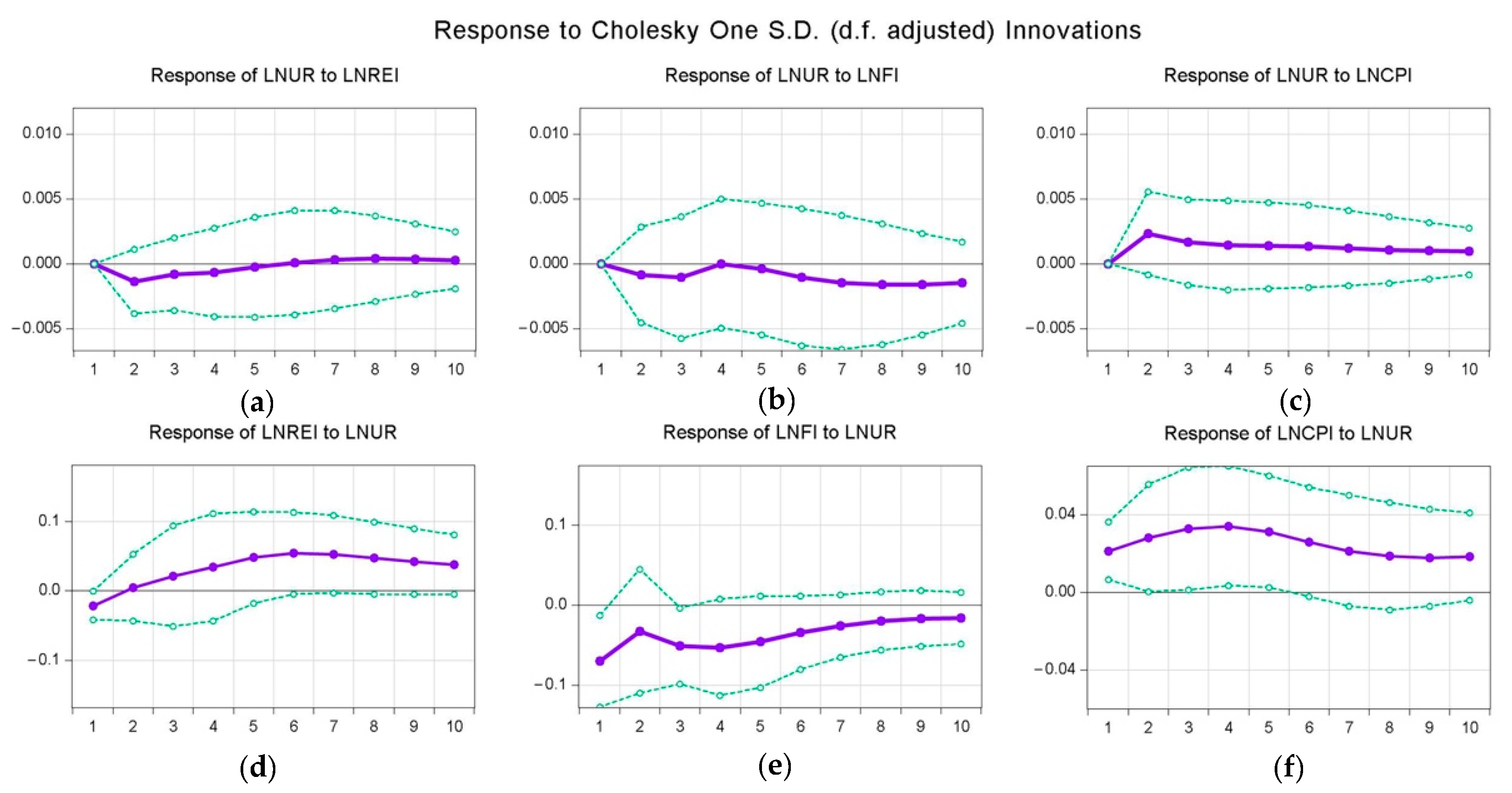
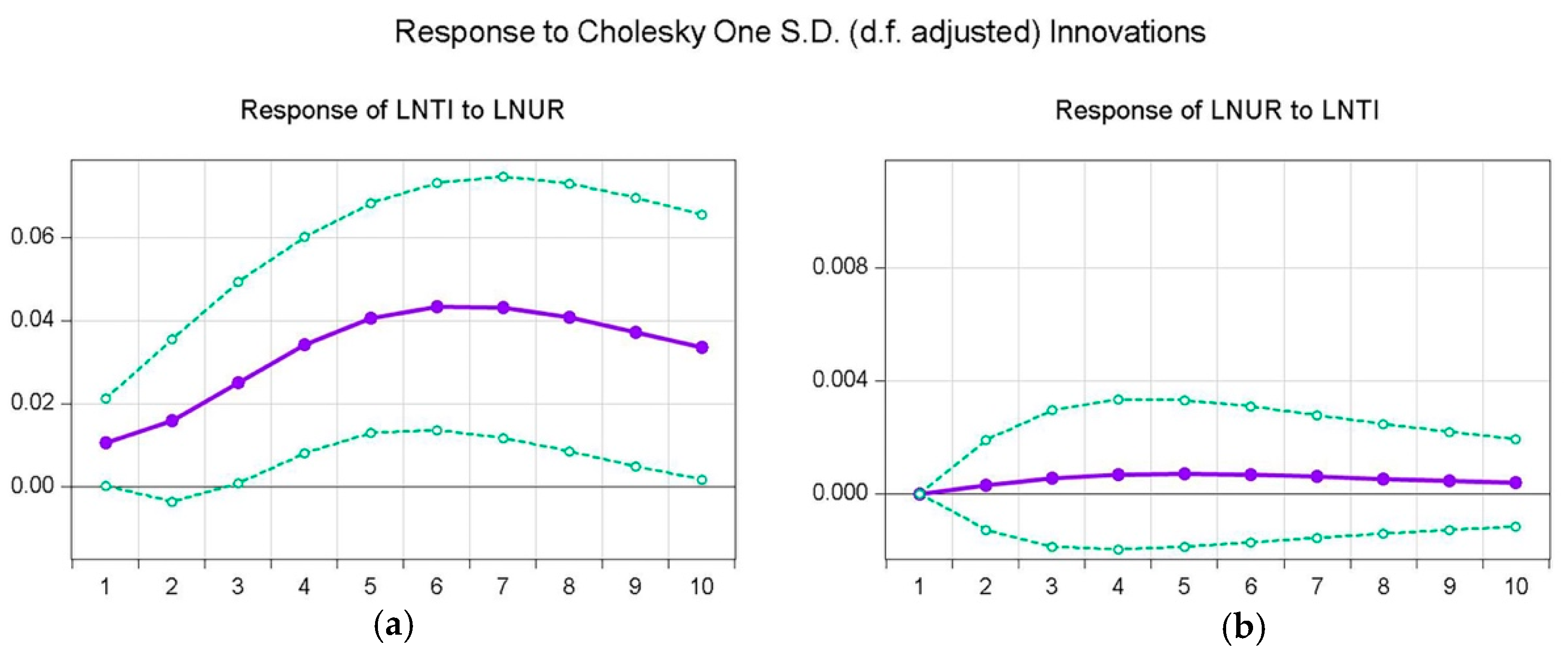
As depicted in Figure 5 and Figure 6, the y-axis shows the impulse response amplitude and direction of different variables.
Moreover, the dotted line represents the positive and negative standard deviation of the impulse response function, and the solid line is considered to be the impulse response function (IRF) image.
Figure 5 presents the dynamic IRF images of urbanization rate, ( l n ( U R t )) and construction project investment, ( l n ( C P I t )), real estate investment ( l n ( R E I t )), and farmers’ investment ( l n ( F I t )). Each curve has its IRF characters, and we focus on combinations related to our research objects, for example, ( l n ( U R t ) , l n ( C P I t )), ( l n ( U R t ) , l n ( R E I t )) and ( l n ( U R t ) , and   l n ( F I t )). There are six combinations. The IRF data can be checked in Appendix A Table A8.
In the first picture in Figure 5, the curve is fluctuated around 0; specifically, l n ( U R t ) is negatively affected by l n ( R E I t ) in the first five periods, and a positive impact is observed in the next five periods.
The second picture illustrates the impact of l n ( U R t ) on l n ( R E I t ). l n ( R E I t ) responds negatively in the first period and then positively after the second period; thus, the increase in the urbanization rate may inevitably promote the growth of real estate investment.
The third curve of Figure 5 depicts the impulse response path of l n ( U R t ) to l n ( F I t ) over time, and the curve is always under the horizontal axis, indicating that l n ( F I t ) has a negative influence on l n ( U R t ) from lags 1 to 10.
The fourth curve of Figure 5 elaborates the impulse response path of l n ( F I t ) to l n ( U R t ) from lags 1 to 10: the curve shows that the l n ( U R t ) has a negative influence on l n ( F I t ) and that the absolute IRF value is higher than that of l n ( U R t ) to l n ( F I t ). This result indicates that the urbanization rate might have more influence on farmers’ investment than the impact from farmers’ investment on urbanization rate. This coincides with the Granger causality test in Section 4.4, that is, urbanization rate has more Granger causality lags with farmers’ investment than those of farmers’ investment with the urbanization rate.
Similarly, the last two images in Figure 5 reflect the same phenomenon of the IRF of two indicators, that is, the two impacts of impulse responses are positive, and the response of l n ( C P I t ) to l n ( U R t ) is smaller than that of l n ( U R t ) to l n ( C P I t ). This result also coincides with the Granger causality test in Section 4.4.
Regarding the Group ( l n U R , l n T I ) IRF results, as shown in Figure 6, both curves are always above the x-axis, and we can easily assess that the response of l n ( T I t ) to l n ( U R t ) is larger than that of l n ( U R t )   to l n ( T I t ). Therefore, we can infer that the urbanization rate’s impact on total investment in fixed assets is greater than total investment in fixed assets’ influence on the urbanization rate. Likewise, this also coincides with the Granger causality test in Section 4.4. The IRF data of the Group ( l n U R , l n T I ) can be checked in Appendix A Table A9.

4.6. Variance Decomposition Analysis

The Variance decomposition (VD) methodology can decompose the variance of a variable in a VAR model into each perturbation term and can help measure the contribution that the shocks have on the variables; thus, we use it to analyze the urbanization rate and other variables as a complementary analysis of the aforementioned methods (Granger causality test and impulse response analysis) in this study.
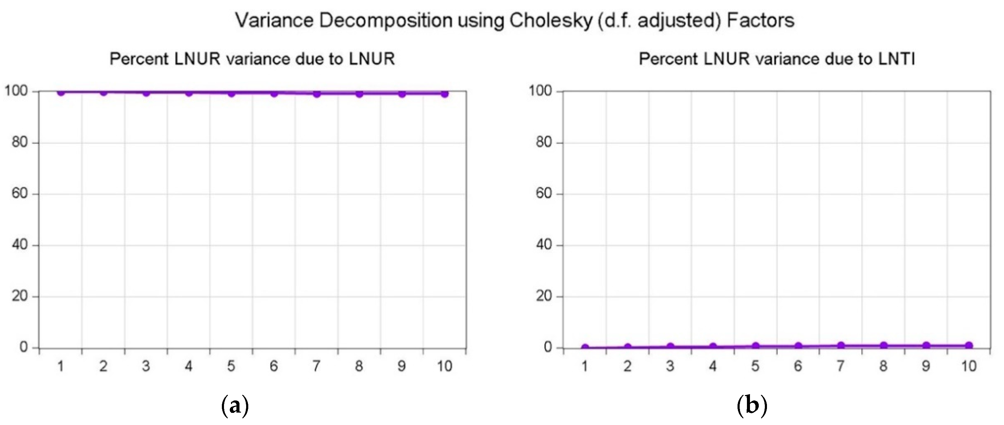
Regarding Group ( l n U R , l n T I ), Figure 7 (for detailed data, see Appendix A Table A10), demonstrates that on impact, 99% of the variation in l n ( U R t ) is accounted for by l n ( U R t ), and l n ( T I t ) only accounts for approximately 1% of shocks.
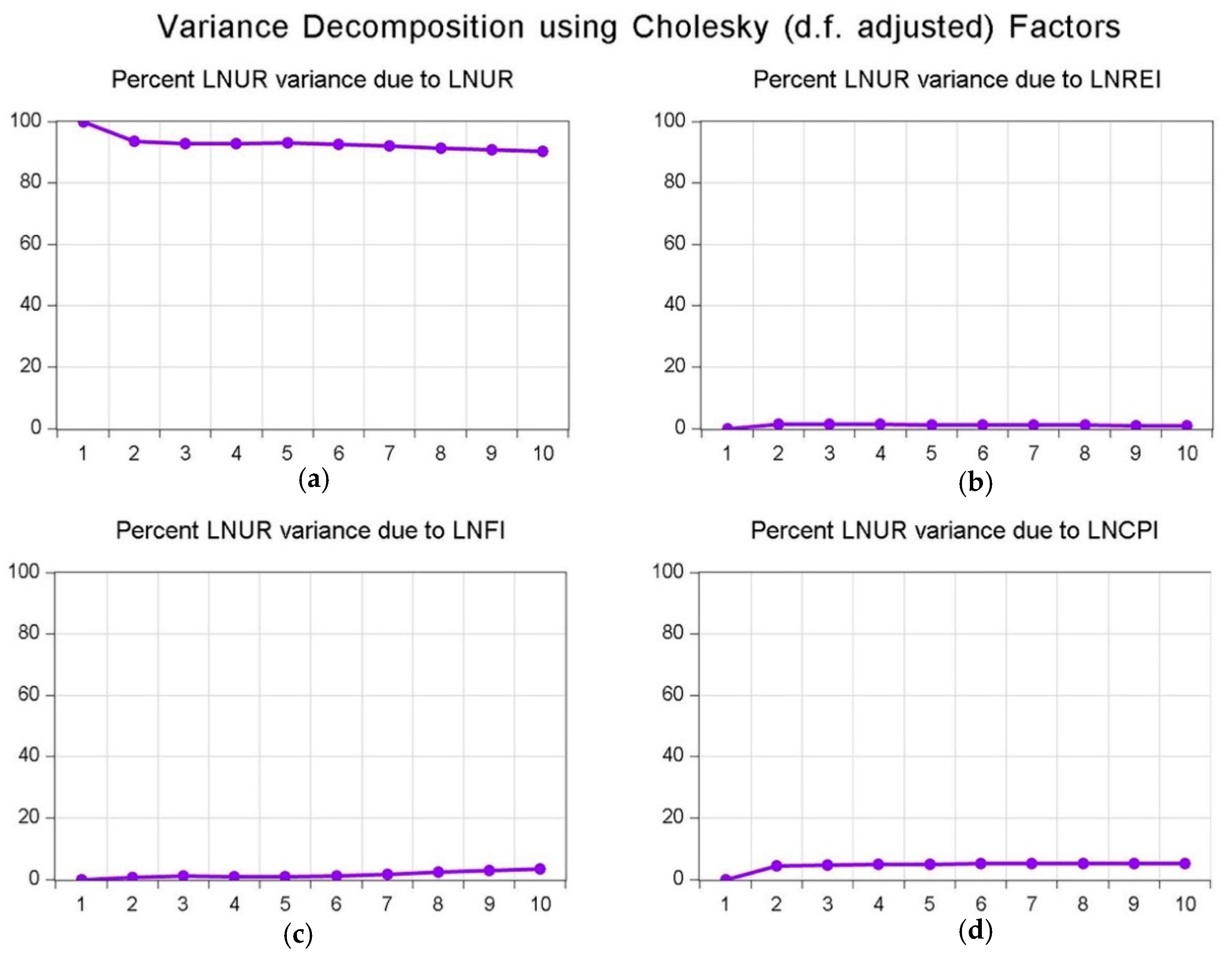
In Figure 8, the variance decomposition results (for detailed data, see Appendix A Table A11), demonstrate that on impact, 90% of the variation in l n ( U R t ) is accounted for by l n ( U R t ), and l n ( C P I t ), l n ( R E I t ), and   l n ( F I t ) account for approximately 5%, 1%, and 2% of shocks, respectively. The result suggests that in the long run, the construction project investment shocks and the farmers’ investment shocks are relatively more important than the real estate investment.

5. Discussion and Conclusions

Shanghai has been experiencing rapid urbanization since China’s opening-up and reform, especially after implementing the strategy of Pudong District development in the 1990s. Additionally, the total investment in fixed assets has substantially changed during the studied period. The purpose of this paper is to investigate the role of total investment in fixed assets in the later stage of urbanization in Shanghai.
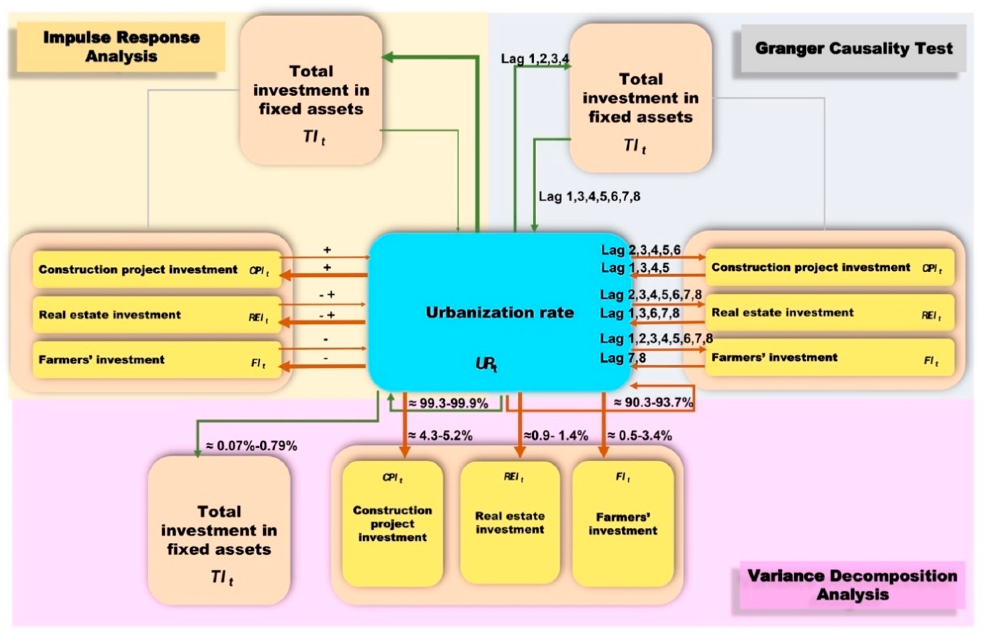
A summary of the main findings of the relationship between the total investment in fixed assets and the urbanization rate is as follows (Figure 9):
  • Both Group ( l n U R , l n F I , l n C P I , and l n R E I ) and Group ( l n U R , l n T I ) have a long-term co-integration relationship among the studied variables, and construction project investment plays an important role in promoting the urbanization rate in the studied period.
  • Granger causality shows that both Group ( l n U R , l n F I , l n C P I , and l n R E I ) and Group ( l n U R , l n T I ) have a bilateral Granger causal relationship; however, the urbanization rate has more Granger causal impact on the studied variable both in Group ( l n U R , l n F I , l n C P I , and l n R E I ) and Group ( l n U R , l n T I ).
  • The impulse response analysis illustrates that the urbanization rate has a positive impact on the total investment in fixed assets in the short term and long term. A similar conclusion is found in [21], that is, government investment policy has substantially affected Egypt and its sustainable development.
  • Variance decomposition analysis reveals that the urbanization rate in Group ( l n U R , l n F I , l n C P I , and l n R E I ) and Group ( l n U R , l n T I ) accounts for the majority of percentage impacts, and the total investment in fixed assets and its three categories contribute a small minority to the urbanization rate.
Based on our co-integration test results, our finding is that construction project investment ( C P I t ) has a higher impact on urbanization rate than real estate investment ( R E I t ) and farmers’ investment ( F I t ), and we can infer that construction project investment ( C P I t ) plays an important role in promoting the urbanization rate in the studied period. This result differs from the conclusion of [13] that real estate is a main driver of urbanization and differs from this statement: “the real estate may have negative influences on the urban sustainable development [21]”.
Moreover, both impulse response analysis results and the variance decomposition results coincide with the co-integration results. The impulse response analysis results show that only the curve of construction project investment ( l n ( C P I t )) to urbanization rate ( l n ( U R t )) is positive: thus the accumulation of the impulse response of l n ( C P I t ) to l n ( U R t ) must be positive, and the variance decomposition results suggest that l n ( C P I t ) has a greater proportion than that two other variables.
Furthermore, we integrated other tests in this paper and found that the three types of total investment in fixed assets have a bilateral relationship with urbanization rate. However, considering the optimal lag length, in the short term (lag = 2,3,4), both construction project investment and real estate investment have a bilateral Granger relationship with urbanization rate, and farmers’ investment has a one-way direction Granger relationship with urbanization rate. This result indicates that in the short term, both the construction project investment and real estate investment are important to urbanization promotion, and the two investments are also affected as the Shanghai urbanization rate increases. Additionally, the urbanization rate affects farmers’ investment, but farmers’ investment does not have an obvious impact on urbanization rate in the short term.
The reason for this finding may be related to the majority of the total investment in fixed assets composition being construction project investment and real estate investment, and the farmers’ investment constitutes less than 8.75% during the studied period.
The finding coincides with that of [57], who found that the urban municipal public infrastructure plays an important role in promoting economic development and that the municipal public infrastructure construction levels and investment efficiency have a close relationship with sustainable socioeconomic development and urbanization.
Notably, construction project investment and real estate investment increase substantially as the Shanghai urbanization rate increases, especially when the main events occur in characteristic years, such as the establishment of Pudong New Area in 1993, the 1998 economic crisis, and the 2010 Shanghai World Expo. The amount of these investments changes during these special times. The urbanization rate also changed in the studied period and the curve of urbanization rate is gentler than that of the other variables.
A similar result is found in Zeng [27], who propose a rational spatial optimization of infrastructure construction and sustainable regional development strategies for improving resource use efficiency, achieving balanced development, and promoting integrated urban–rural development.
In addition, considering the optimal lag length, in the short term (lag = 8), farmers’ investment has a bilateral Granger causal relationship with urbanization rate. Notably, as urbanization rate increases, the urban area would provide an increasing amount of help to the rural area, although as the percentage of farmers’ investment in the total investment in fixed assets was decreasing, the amount of the farmers’ investment was increasing; therefore, rural area construction would increase. This phenomenon coincides with the recent “rural revitalization” in China.

6. Policy Implication

This study contributes a novel insight into the current reality of the urbanization rate and total investment in fixed assets. In summary, according to our results, in terms of the related policies, to strengthen the healthy urbanization development in Shanghai, improve the rational total investment in fixed assets of Shanghai, and maintain coordinated rapid economic growth in manners similar to green investment [34], sustainable urban infrastructure development [35], and UGI planning [36], eco-system services and integrated urban planning [58], we suggest that policy makers should prioritize strategy policy, economy policy, industrial policy, and population policy. Based on our research, our policy suggestions as follows:
  • Strengthen the rational total investment in fixed assets. According to our results, the total investment in fixed assets has a one-direction Granger relationship with urbanization rate and a bilateral Granger relationship in the long term. Notably, urbanization is a process that needs time to comply with economic factors, such as the total investment in fixed assets. Thus, the city would not benefit from the higher urbanization rate. Similarly, the total investment in fixed assets also needs a process that would convert its investment into related beneficial interests of the city. Therefore, a rational investment strategy is necessary to ensure the healthy development of urbanization through, for example, conceptual infrastructure planning and investment project appraisal schemes. A similar implication can be found in [57].
  • Set a more flexible policy on construction project investment. Generally, construction project investment is a critical factor that plays a substantial role as a drive of urban development. In addition, our results demonstrate a one-way Granger relationship between construction project investment and urbanization rate. Therefore, policymakers must balance the two indicators, for example, the related population policy and construction project investment policy, which can be implemented according to the current condition to solve urban problems (i.e., gentrification, polarization, and urban renewal) caused by urbanization [2].
  • More rationally guide the development of the real estate industry. Theoretically, based on the characteristics of the other countries’ urbanization experience, urbanization can be divided into four stages: initial, acceleration, deceleration, and stable.
    Similarly, the development of the real estate industry follows similar laws of urbanization development, summarized as four stages: formation, growth, maturity, and decline. However, the relationship between urbanization and the real estate industry should be harmonious, or it may cause serious economic problems. Notably, the real estate industry has developed rapidly since the commercial housing reform in Shanghai in 1998. However, the real estate industry has always been the economic pillar of Shanghai and has been criticized for its “excessively high housing price,” the “real estate bubble,” and other problems of the society. Moreover, according to our research, there is a bilateral direction of Granger causality between the real estate industry and urbanization, indicating that the two factors have a close relationship. Therefore, Shanghai should guide the rational development of the real estate industry in the later stage of urbanization. More specifically, the government should coordinate land financing policy [12] and eliminate the negative externalities of the policy, for example, the polarization effect and high housing prices; thus, the government must more practically manage the related social, economic, or environmental problems caused by real estate investment.
  • Promote rural revitalization and coordinate the development of urbanization through scientific planning.
Urban planning should be in accordance with the requirements of building a harmonious society and the coordination of development between different regions and between urban and rural areas. Additionally, urban planning should make overall plans for economic and social aspects and construction.
Thus, Shanghai should accurately understand the urbanization progress to avoid excessive urban sprawl. Furthermore, regarding the amount of total investment in fix assets, Shanghai should make it compatible with urbanization development and the current level of economic development. Related policy should be implemented to balance the relationship between the two factors.

Author Contributions

Conceptualization, Y.L., C.W. and K.D.; methodology, Y.L. and W.Z.; software, Y.L. and C.C.; validation, Y.L., C.W. and K.D.; formal analysis, Y.L., C.W. and K.D.; investigation, Y.L., C.W. and K.D.; resources, Y.L., C.W. and K.D.; data curation, Y.L. and C.C.; writing—original draft preparation, Y.L., C.W. and K.D.; writing—review and editing, Y.L., W.Z., C.W. and K.D.; visualization, Y.L. and W.Z.; supervision, Y.L. and W.Z.; project administration, Y.L. and W.Z.; funding acquisition, Y.L., W.Z. and K.D. All authors have read and agreed to the published version of the manuscript.

Funding

This research was funded by National Natural Science Foundation of China (Grant No.61803100), Starting funding of “100 Youth Talents” Project in Guangdong University of Technology (Grant No. 220413735), Hangzhou Planning Program of Philosophy and Social Science (Grant No.M19JC052), and Guangdong Province Undergraduate Education Quality of Universities and The Specialized Project of Urban and Rural Planning Education Reform Project (Grant No. Guangdong Education Letter [2018] 179).

Institutional Review Board Statement

Not applicable.

Informed Consent Statement

Not applicable.

Data Availability Statement

The data presented in this study are openly available in the website: http://tjj.sh.gov.cn/ accessed on 23 March 2021.

Acknowledgments

We greatly thanks to Yun Huang for the contributions for this paper.

Conflicts of Interest

The authors declare no conflict of interest.

Appendix A

  • Unit root test.
    • ADF test
      Table A1. ADF test.
      Table A1. ADF test.
      Include in Test Equation VariablesADF Test StatisticTest Critical ValueProb.*
      (5% Level)
      Level
      Intercept1ln(TI)−2.974150−3.0123630.0539
      2ln(CPI)−3.007464−3.0123630.0505
      3ln(REI)−1.420050−3.0048610.5538
      4ln(FI)−1.901596−2.9762630.3266
      5ln(UR)−1.355025−2.9762630.5888
      Intercept and trend1ln(TI)−0.252700−3.6449630.9865
      2ln(CPI)−1.271979−3.6449630.8668
      3ln(REI)−4.679380−3.5950260.0048
      4ln(FI)−2.459441−3.5875270.3437
      5ln(UR)−0.067273−3.5875270.9928
      None1ln(TI)3.398008−1.9564060.9995
      2ln(CPI)0.778335−1.9544140.8754
      3ln(REI)2.492405−1.9564060.9953
      4ln(FI)−1.093929−1.9538580.2413
      5ln(UR)2.789532−1.9538580.9979
      First difference
      Intercept1ln(TI)−6.059505−2.9980640.0000
      2ln(CPI)−2.094011−2.9810380.2484
      3ln(REI)−8.306588−2.9980640.0000
      4ln(FI)−5.777930−2.9810380.0001
      5ln(UR)−2.093889−2.9862250.2485
      Intercept and trend1ln(TI)−4.879820−3.6449630.0043
      2ln(CPI)−4.235406−3.6449630.0159
      3ln(REI)−6.881178−3.6220330.0001
      4ln(FI)−5.746140−3.5950260.0004
      5ln(UR)−2.566373−3.6032020.2969
      None1ln(TI)−1.380192−1.9544140.1516
      2ln(CPI)−1.808925−1.9544140.0676
      3ln(REI)−1.989104−1.9544140.0465
      4ln(FI)−5.843456−1.9544140.0000
      5ln(UR)−1.668758−1.9550200.0892
      * MacKinnon (1996) one-sided p-values.
    • PP test
      Table A2. PP test.
      Table A2. PP test.
      Include in Test Equation VariablesPP Test StatisticTest Critical ValueProb. *
      (5% Level)
      Level
      Intercept1ln(TI)−3.312157−2.9762630.0243
      2ln(CPI)−3.682527−2.9762630.0104
      3ln(REI)−2.661924−2.9762630.0937
      4ln(FI)−1.860863−2.9762630.3447
      5ln(UR)−1.307643−2.9762630.6111
      Intercept and trend1ln(TI)−2.397368−3.5875270.3725
      2ln(CPI)−2.393708−3.5875270.3742
      3ln(REI)−1.940834−3.5875270.6059
      4ln(FI)−2.459441−3.5875270.3437
      5ln(UR)−0.327360−3.5875270.9853
      None1ln(TI)2.056535−1.9538580.9883
      2ln(CPI)1.703675−1.9538580.9754
      3ln(REI)1.134348−1.9538580.9293
      4ln(FI)−1.137367−1.9538580.2258
      5ln(UR)2.473166−1.9538580.9955
      First difference
      Intercept1ln(TI)−1.982617−2.9810380.2921
      2ln(CPI)−2.168164−2.9810380.2218
      3ln(REI)−2.562258−2.9810380.1134
      4ln(FI)−5.982451−2.9810380.0000
      5ln(UR)−4.333654−2.9810380.0023
      Intercept and trend1ln(TI)−2.624646−3.5950260.2732
      2ln(CPI)−2.640510−3.5950260.2670
      3ln(REI)−3.060382−3.5950260.1362
      4ln(FI)−5.963815−3.5950260.0003
      5ln(UR)−4.602260−3.5950260.0058
      None1ln(TI)−1.579302−1.9544140.1058
      2ln(CPI)−1.765214−1.9544140.0738
      3ln(REI)−2.158700−1.9544140.0321
      4ln(FI)−5.890789−1.9544140.0000
      5ln(UR)−3.550310−1.9544140.0010
      * MacKinnon (1996) one-sided p-values.
    • DF GLS test
      Table A3. DF GLS test.
      Table A3. DF GLS test.
      Include in Test Equation VariablesDF GLS Test StatisticTest Critical Value
      (5% Level)
      Level
      Intercept1ln(TI)−0.131325−1.95502
      2ln(CPI)−1.086410−1.954414
      3ln(REI)−0.735425−1.955020
      4ln(FI)−1.624687−1.953858
      5ln(UR)−1.150360−1.955020
      Intercept and trend1ln(TI)−4.177963−3.190000
      2ln(CPI)−3.193654−3.190000
      3ln(REI)−2.093001−3.190000
      4ln(FI)−2.676590−3.190000
      5ln(UR)−1.442210−3.190000
      First difference
      Intercept1ln(TI)−1.744151−1.954414
      2ln(CPI)−2.116516−1.954414
      3ln(REI)−9.221668−1.956406
      4ln(FI)−5.899968−1.954414
      5ln(UR)−1.968365−1.955020
      Intercept and trend1ln(TI)−5.179672−3.190000
      2ln(CPI)−4.189617−3.190000
      3ln(REI)−2.770603−3.190000
      4ln(FI)−5.980730−3.190000
      5ln(UR)−2.593204−3.190000
    • KPSS test
      Table A4. KPSS test.
      Table A4. KPSS test.
      Include in Test Equation VariablesKPSS Test Statistic
      (LM-Stat.)
      Test Critical Value
      (5% Level)
      Level
      Intercept1ln(TI)0.6356110.463000
      2ln(CPI)0.6097670.463000
      3ln(REI)0.5863190.463000
      4ln(FI)0.5523660.463000
      5ln(UR)0.6304470.463000
      Intercept and trend1ln(TI)0.1481300.146000
      2ln(CPI)0.1557060.146000
      3ln(REI)0.1498420.146000
      4ln(FI)0.1109500.146000
      5ln(UR)0.1166010.146000
      First difference
      Intercept1ln(TI)0.3265060.463000
      2ln(CPI)0.3484730.463000
      3ln(REI)0.2834570.463000
      4ln(FI)0.1462400.463000
      5ln(UR)0.2861960.463000
      Intercept and trend1ln(TI)0.0902250.146000
      2ln(CPI)0.0830300.146000
      3ln(REI)0.0749520.146000
      4ln(FI)0.0941820.146000
      5ln(UR)0.1719650.146000
  • VAR model stability test
    • LNUR and LNREI, LNFI, LNCPI
      Figure A1. Inverse Roots of AR Characteristic Polynomial of LNUR and LNREL, LNFI, LNCPI.
      Figure A1. Inverse Roots of AR Characteristic Polynomial of LNUR and LNREL, LNFI, LNCPI.
      Sustainability 13 03661 g0a1
    • LNUR and LNTI
      Figure A2. Inverse Roots of AR Characteristic Polynomial of LNUR and LNTI.
      Figure A2. Inverse Roots of AR Characteristic Polynomial of LNUR and LNTI.
      Sustainability 13 03661 g0a2
  • Lag length Criteria
    Table A5. The optimal lag length test results.
    Table A5. The optimal lag length test results.
    Endogenous Variables: LNUR LNREI LNFI LNCPI
    LagLogLLRFPEAICSCHQ
    0107.3996NA2.13 × 10−9−8.616631−8.420289−8.564541
    1190.6542131.81988.03 × 10−12−14.22118−13.23947−13.96073
    2224.776142.65236 *2.02 × 10−12−15.73134−13.96426 *−15.26253
    3247.182220.538951.70 × 10−12 *−16.26518−13.71273−15.58802
    4273.551915.382331.74 × 10−12−17.12933*−13.79151−16.24380 *
    Endogenous variables: LNUR LNTI
    069.43158NA4.04 × 10−6−6.743158−6.643585−6.72372
    1117.728982.105424.84 × 10−8−11.17289−10.87417−11.11458
    2126.037912.46350 *3.20 × 10−8 *−11.60379−11.10592 *−11.5066
    3128.77883.5632233.78 × 10−8−11.47788−10.78087−11.34182
    4131.05462.5034104.85 × 10−8−11.30546−10.40931−11.13053
    5136.76275.1372054.67 × 10−8−11.47627−10.38096−11.26245
    6137.78660.7167487.90 × 10−8−11.17866−9.884206−10.92597
    7145.89184.0526237.75 × 10−8−11.58918−10.09558−11.29762
    8157.90173.6029757.24 × 10−8−12.39017*−10.69743−12.05973 *
    Endogenous variables: LNCPI LNUR
    071.68151NA3.23 × 10−6−6.968151−6.868578−6.948713
    1109.418964.153551.11 × 10−7−10.34189−10.04317−10.28358
    2118.892214.21001 *6.54 × 10−8 *−10.88922−10.39136 *−10.79203
    3122.60844.8310307.00 × 10−8−10.86084−10.16383−10.72478
    4127.22595.0792357.11 × 10−8−10.92259−10.02643−10.74765
    5132.64274.8751377.06 × 10−8−11.06427−9.968966−10.85046
    6134.50601.3042671.10 × 10−7−10.8506−9.556144−10.5979
    7136.51021.0021041.98 × 10−7−10.65102−9.157418−10.35945
    8153.09504.9754591.17 × 10−7−11.90950 *−10.21676−11.57906 *
    Endogenous variables: LNUR LNFI
    050.94417NA2.57 × 10−5−4.894417−4.794844−4.87498
    183.3477955.086161.51 × 10−6−7.734779−7.43606−7.676466
    284.987802.4600081.94 × 10−6−7.49878−7.000914−7.401591
    387.319353.0310192.39 × 10−6−7.331935−6.634923−7.195871
    488.615141.4253663.38 × 10−6−7.061514−6.165355−6.886574
    592.246683.2683844.01 × 10−6−7.024668−5.929362−6.810853
    6107.430610.628731.65 × 10−6−8.143058−6.848606−7.890368
    7125.02438.7968776.24 × 10−7−9.502434−8.008835−9.210868
    8160.304310.58400*5.69 × 10−8 *−12.63043 *−10.93769 *−12.29999 *
    Endogenous variables: LNUR LNREI
    053.23147NA2.04 × 10−5−5.123147−5.023573−5.103709
    1107.070191.525681.40 × 10−7−10.10701−9.808291−10.0487
    2112.51538.1677301.24 × 10−7−10.25153−9.75366−10.15434
    3117.72686.7749921.14 × 10−7−10.37268−9.675666−10.23661
    4119.73442.2084021.50 × 10−7−10.17344−9.277284−9.998503
    5136.979715.52072 *4.57 × 10−8−11.49797−10.40266−11.28415
    6143.58974.6270384.42 × 10−8−11.75897−10.46452−11.50628
    7148.77492.5925695.81 × 10−8−11.87749−10.38389−11.58592
    8175.38017.9815621.26 × 10−8 *−14.13801 *−12.44526 *−13.80757 *
    * indicates lag order selected by the criterion. LR: sequential modified LR test statistic (each test at 5% level). FPE: Final prediction error. AIC: Akaike information criterion. SC: Schwarz information criterion. HQ: Hannan-Quinn information criterion
  • JJ test
    Table A6. Co-integration test.
    Table A6. Co-integration test.
    Variables GroupJJ Co-Integration
    Configuration
    Co-Integration Equation
    Number
    Log Likelihood Value
    Trace TestMax-Eigenvalue Test
    LNUR and LNTIno intercept or trend in test VAR; Lags interval (in first differences): 1 to 111152.0092
    LNUR and LNCPI, LNREI, LNFIno intercept or trend in test VAR; Lags interval (in first differences): 1 to 111193.6514
  • Granger causality test
    Table A7. Granger causality test result.
    Table A7. Granger causality test result.
    Lag LengthUrbanization Rate and Total Investment in Fixed AssetsUrbanization Rate and Construction Project InvestmentUrbanization Rate and Real Estate InvestmentUrbanization Rate and Farmers’ Investment
    Null HypothesisF-Statisticp-ValueAccept/
    Reject
    ConclusionNull HypothesisF-Statisticp-ValueAccept/
    Reject
    ConclusionNull HypothesisF-Statisticp-ValueAccept/
    Reject
    ConclusionNull HypothesisF-Statisticp-ValueAccept/
    Reject
    Conclusion
    1 T I t ≠> U R t 0.950.34R T I t U R t C P I t ≠> U R t 1.690.21R C P I t U R t R E I t ≠> U R t 0.770.39R R E I t U R t U R t ≠> F I t 5.270.03R U R t F I t
    1 U R t ≠> T I t 0.80.38R U R t T I t U R t ≠> C P I t 0.50.49A U R t ≠> C P I t U R t ≠> R E I t 0.190.66A U R t ≠> R E I t F l t ≠> U R t 0.040.84A F l t ≠> U R t
    2 T I t ≠> U R t 0.140.86A T I t ≠> U R t C P I t ≠> U R t 0.450.64A C P I t ≠> U R t R E I t ≠> U R t 0.340.71A R E I t U R t U R t ≠> F I t 3.020.07R U R t F I t
    2 U R t ≠> T I t 9.370R U R t T I t U R t ≠> C P I t 3.890.04R U R t C P I t U R t ≠> R E I t 3.660.04R U R t R E I t F l t ≠> U R t 0.090.92A F l t ≠> U R t
    3 T I t ≠> U R t 1.90.16R T I t U R t C P I t ≠> U R t 1.630.22R C P I t U R t R E I t ≠> U R t 0.660.59R R E I t U R t U R t ≠> F I t 2.460.1R U R t F I t
    3 U R t ≠> T l t 7.230R U R t T I t U R t ≠> C P I t 4.860.01R U R t     C P I t U R t ≠> R E I t 2.230.12R U R t R E I t F l t ≠> U R t 0.230.88A F l t ≠> U R t
    4 T I t ≠> U R t 1.340.3R T I t U R t C P I t ≠> U R t 1.290.32R C P I t U R t R E I t ≠> U R t 0.430.78A R E I t ≠> U R t U R t ≠> F I t 2.820.06R U R t F I t
    4 U R t ≠> T l t 1.370.29R U R t T l t U R t ≠> C P I t 1.690.2R U R t C P I t U R t ≠> R E I t 14.20R U R t R E I t F I t ≠> U R t 0.250.91A F I t ≠> U R t
    5 T I t ≠> U R t 0.750.6R T I t U R t C P I t ≠> U R t 0.970.47R C P I t U R t R E I t ≠> U R t 0.450.81A R E I t ≠> U R t U R t ≠> F I t 1.60.23R U R t F I t
    5 U R t ≠> T I t 0.550.74A U R t ≠> T I t U R t ≠> C P I t 1.190.37R U R t     C P I t U R t ≠> R E I t 6.620R U R t R E I t F I t ≠> U R t 0.160.97A F I t ≠> U R t
    6 T I t ≠> U R t 0.780.61R T I t U R t C P I t ≠> U R t 0.520.78A C P I t ≠> U R t R E I t ≠> U R t 1.080.44R R E I t U R t U R t ≠> F I t 5.020.02R U R t F I t
    6 U R t ≠> T I t 0.440.83A U R t ≠> T I t U R t ≠> C P I t 1.050.45R U R t     C P I t U R t ≠> R E I t 2.50.11R U R t R E I t F I t ≠> U R t 0.570.75A F I t ≠> U R t
    7 T I t ≠> U R t 0.940.54R T I t ≥ UR C P I t ≠> 0.30.93A C P I t ≠> R E I t ≠> U R t 0.920.55R R E I t U R t U R t ≠> F I t 6.060.02R U R t F I t
    7 U R t ≠> T I t 0.580.75A U R t ≠> T I t U R t ≠> C P I t 0.590.75A U R t ≠> C P I t U R t ≠> R E I t 2.670.13R U R t R E I t F I t ≠> U R t 1.630.28R F I t U R t
    8 T I t ≠> U R t 0.930.59R T I t ≥ UR C P I t ≠> U R t 0.460.83A C P I t ≠> U R t R E I t ≠> U R t 2.790.22R R E I t U R t U R t ≠> F I t 10.080.04R U R t F I t
    8 U R t ≠> T I t 0.260.94A U R t ≠> T I t U R t ≠> C P I t 0.340.9A U R t ≠> C P I t U R t ≠> R E I t 11.010.04R U R t R E I t F I t ≠> U R t 3.360.17R F I t U R t
  • Impulse response function analysis
    Table A8. Impulse response function analysis result of Group ( l n U R , l n F I , l n C P I and l n R E I ).
    Table A8. Impulse response function analysis result of Group ( l n U R , l n F I , l n C P I and l n R E I ).
    Response of LNUR:
    PeriodLNURLNREILNFILNCPI
    10.0080150.0000000.0000000.000000
    (0.00111)(0.00000)(0.00000)(0.00000)
    20.007424−0.001344−0.0008350.002355
    (0.00229)(0.00124)(0.00185)(0.00160)
    30.006740−0.000817−0.0010570.001661
    (0.00226)(0.00141)(0.00236)(0.00166)
    40.005870−0.0006692.39E−060.001433
    (0.00218)(0.00171)(0.00249)(0.00172)
    50.005507−0.000256−0.0003880.001391
    (0.00208)(0.00193)(0.00254)(0.00167)
    60.0049879.76E−05−0.0010330.001346
    (0.00211)(0.00201)(0.00265)(0.00158)
    70.0045290.000333−0.0014450.001203
    (0.00207)(0.00190)(0.00259)(0.00146)
    80.0041910.000402−0.001590.001090
    (0.00200)(0.00165)(0.00233)(0.00129)
    90.0039530.000366−0.0015810.001016
    (0.00193)(0.00135)(0.00195)(0.00109)
    100.0037590.000277−0.0014540.000963
    (0.00189)(0.00109)(0.00157)(0.00090)
    Response of LNREI:
    PeriodLNURLNREILNFILNCPI
    1−0.0213520.0500060.0000000.000000
    (0.01024)(0.00693)(0.00000)(0.00000)
    20.0047240.055465−0.0714060.050022
    (0.02428)(0.02024)(0.01846)(0.01266)
    30.0215780.049850−0.1043690.061358
    (0.03640)(0.02913)(0.03148)(0.02220)
    40.0342520.034144−0.0766690.049433
    (0.03881)(0.02893)(0.03889)(0.02755)
    50.0481980.019811−0.0456060.033325
    (0.03291)(0.02846)(0.03992)(0.02656)
    60.0544880.011126−0.0292320.018094
    (0.02957)(0.02910)(0.03853)(0.02476)
    70.0527760.006943−0.0221260.005269
    (0.02800)(0.02850)(0.03916)(0.02311)
    80.0474390.004342−0.018585−0.002232
    (0.02600)(0.02578)(0.03815)(0.02179)
    90.0419970.001767−0.016069−0.003654
    (0.02363)(0.02184)(0.03352)(0.01967)
    100.037861−0.001002−0.012863−0.00066
    (0.02151)(0.01822)(0.02756)(0.01649)
    Response of LNFI:
    PeriodLNURLNREILNFILNCPI
    1−0.070103−0.0092860.1359640.000000
    (0.02844)(0.02670)(0.01885)(0.00000)
    2−0.0327950.0347580.009469−0.007008
    (0.03859)(0.02216)(0.03418)(0.02987)
    3−0.0511160.043485−0.0504−0.012088
    (0.02356)(0.02032)(0.03346)(0.02007)
    4−0.0528880.039885−0.058855−0.025699
    (0.03005)(0.02250)(0.03215)(0.02133)
    5−0.045860.022481−0.040059−0.024572
    (0.02866)(0.02281)(0.03554)(0.02250)
    6−0.0344990.005305−0.019324−0.017462
    (0.02281)(0.02208)(0.03446)(0.02165)
    7−0.025916−0.0075930.002268−0.009639
    (0.01949)(0.02136)(0.02998)(0.01886)
    8−0.019954−0.0138410.018508−0.003767
    (0.01816)(0.02021)(0.02832)(0.01626)
    9−0.01687−0.0140110.025670−0.00043
    (0.01738)(0.01770)(0.02747)(0.01580)
    10−0.016266−0.0100690.0243400.000185
    (0.01604)(0.01462)(0.02505)(0.01563)
    Response of LNCPI:
    PeriodLNURLNREILNFILNCPI
    10.021433−0.004447−0.011310.032548
    (0.00743)(0.00679)(0.00657)(0.00451)
    20.028201−0.006838−0.0056610.043433
    (0.01383)(0.01037)(0.01248)(0.00998)
    30.032984−0.0040540.0037830.037967
    (0.01573)(0.01118)(0.01579)(0.01157)
    40.0342500.0017980.0027530.026742
    (0.01538)(0.01204)(0.01707)(0.01203)
    50.0313420.008494−0.0073330.013502
    (0.01436)(0.01292)(0.01718)(0.01153)
    60.0260880.012557−0.0175620.002152
    (0.01413)(0.01363)(0.01771)(0.01083)
    70.0214560.012505−0.023114−0.004478
    (0.01429)(0.01345)(0.01818)(0.01066)
    80.0187720.008894−0.022676−0.005843
    (0.01380)(0.01229)(0.01776)(0.01060)
    90.0180180.003566−0.017313−0.003345
    (0.01252)(0.01075)(0.01602)(0.00986)
    100.018456−0.001428−0.0096030.000901
    (0.01125)(0.00948)(0.01362)(0.00841)
    Cholesky Ordering: LNUR LNREI LNFI LNCPI. Standard Errors: Analytic, The standard errors are marked in parentheses.
    Table A9. Impulse response function analysis result of Group ( l n U R , l n T I ).
    Table A9. Impulse response function analysis result of Group ( l n U R , l n T I ).
    Response of LNUR:
    PeriodLNURLNTI
    10.0077950.000000
    (0.00108)(0.00000)
    20.0075750.000307
    (0.00211)(0.00079)
    30.0070270.000552
    (0.00218)(0.00121)
    40.0065890.000687
    (0.00220)(0.00133)
    50.0062450.000722
    (0.00228)(0.00129)
    60.0059520.000687
    (0.00237)(0.00120)
    70.0056820.000614
    (0.00242)(0.00109)
    80.0054150.000531
    (0.00244)(0.00098)
    90.0051440.000456
    (0.00243)(0.00087)
    100.0048710.000399
    (0.00242)(0.00077)
    Response of LNTI:
    PeriodLNURLNTI
    10.0106480.025808
    (0.00527)(0.00358)
    20.0159470.035379
    (0.00980)(0.00567)
    30.0250870.033296
    (0.01215)(0.00717)
    40.0341560.025147
    (0.01302)(0.00780)
    50.0405340.015488
    (0.01384)(0.00782)
    60.0433940.007214
    (0.01488)(0.00782)
    70.0431300.001613
    (0.01575)(0.00797)
    80.040723−0.001224
    (0.01618)(0.00799)
    90.037249−0.001894
    (0.01621)(0.00764)
    100.033580−0.001234
    (0.01599)(0.00694)
    Cholesky Ordering: LNUR LNTI. Standard Errors: Analytic, The standard errors are marked in parentheses.
  • Variance decomposition analysis
    Table A10. Variance decomposition analysis result of Group ( l n U R , l n T I ).
    Table A10. Variance decomposition analysis result of Group ( l n U R , l n T I ).
    Variance Decomposition of LNUR:
    PeriodS.E.LNURLNTI
    10.007795100.00000.000000
    20.01087499.920330.079668
    30.01295999.762760.237236
    40.01455499.589020.410983
    50.01585499.445950.554046
    60.01694899.350940.649055
    70.01788699.299440.700557
    80.01869599.278120.721876
    90.01939599.273930.726070
    100.02000199.277560.722442
    Cholesky Ordering: LNUR LNTI.
    Table A11. Variance decomposition analysis result of Group ( l n U R , l n F I , l n C P I and l n R E I ).
    Table A11. Variance decomposition analysis result of Group ( l n U R , l n F I , l n C P I and l n R E I ).
    Variance Decomposition of LNUR:
    PeriodS.E.LNURLNREILNFILNCPI
    10.008015100.00000.0000000.0000000.000000
    20.01128793.684451.4168770.5468924.351780
    30.01331892.902391.3944561.0226644.680485
    40.01464092.958741.3629490.8463294.831987
    50.01571093.013511.2101280.7960654.980294
    60.01657092.667791.0912391.1042835.136685
    70.01728492.040111.0400781.7139075.205907
    80.01789391.362001.0209462.3884555.228599
    90.01842490.773051.0023542.9888635.235735
    100.01888790.345070.9754133.4368235.242690
    Cholesky Ordering: LNUR LNREI LNFI LNCPI.

References

  1. Chaolin, G. Urbanization. In International Encyclopedia of Human Geography, 2nd ed.; Kobayashi, A., Ed.; Elsevier: Oxford, UK, 2020; pp. 141–153. [Google Scholar]
  2. Guan, X.; Wei, H.; Lu, S.; Dai, Q.; Su, H. Assessment on the urbanization strategy in China: Achievements, challenges and reflections. Habitat. Int. 2018, 71, 97–109. [Google Scholar] [CrossRef]
  3. Northam, R.M.J.R. Urban Geography; Wiley: Hoboken, NJ, USA, 1979; Volume 23, pp. 430–444. [Google Scholar]
  4. Chu, Y.-W. China’s new urbanization plan: Progress and structural constraints. Cities 2020, 103, 102736. [Google Scholar] [CrossRef]
  5. Perry, D.C. Infrastructure Investment. In International Encyclopedia of the Social & Behavioral Sciences, 2nd ed.; Wright, J.D., Ed.; Elsevier: Oxford, UK, 2015; pp. 116–118. [Google Scholar]
  6. Cheng, M.; Lu, Y. Investment efficiency of urban infrastructure systems: Empirical measurement and implications for China. Habitat. Int. 2017, 70, 91–102. [Google Scholar] [CrossRef]
  7. Tian, L.; Ge, B.; Li, Y. Impacts of state-led and bottom-up urbanization on land use change in the peri-urban areas of Shanghai: Planned growth or uncontrolled sprawl? Cities 2017, 60, 476–486. [Google Scholar] [CrossRef]
  8. Maparu, T.S.; Mazumder, T.N. Transport infrastructure, economic development and urbanization in India (1990–2011): Is there any causal relationship? Transp. Res. Part A Policy Pract. 2017, 100, 319–336. [Google Scholar] [CrossRef]
  9. Grafe, F.-J.; Mieg, H.A. Connecting financialization and urbanization: The changing financial ecology of urban infrastructure in the UK. Reg. Stud. Reg. Sci. 2019, 6, 496–511. [Google Scholar] [CrossRef]
  10. Shannon, M.; Otsuki, K.; Zoomers, A.; Kaag, M. Sustainable Urbanization on Occupied Land? The politics of infrastructure development and resettlement in Beira city, Mozambique. Sustainability 2018, 10, 3123. [Google Scholar] [CrossRef] [Green Version]
  11. Tang, Y.; Xu, J.; Zhang, X. China’s investment and rate of return on capital revisited. J. Asian Econ. 2017, 49, 12–25. [Google Scholar] [CrossRef]
  12. Guo, S.; Shi, Y. Infrastructure investment in China: A model of local government choice under land financing. J. Asian Econ. 2018, 56, 24–35. [Google Scholar] [CrossRef]
  13. Cai, Z.; Liu, Q.; Cao, S. Real estate supports rapid development of China’s urbanization. Land Use Policy 2020, 95, 104582. [Google Scholar] [CrossRef]
  14. Gao, X.; Zhang, A.; Sun, Z. How regional economic integration influence on urban land use efficiency? A case study of Wuhan metropolitan area, China. Land Use Policy 2020, 90, 104329. [Google Scholar] [CrossRef]
  15. Wu, Y.; Heerink, N. Foreign direct investment, fiscal decentralization and land conflicts in China. China Econ. Rev. 2016, 38, 92–107. [Google Scholar] [CrossRef]
  16. Vongpraseuth, T.; Choi, C.G. Globalization, foreign direct investment, and urban growth management: Policies and conflicts in Vientiane, Laos. Land Use Policy 2015, 42, 790–799. [Google Scholar] [CrossRef]
  17. Lin, B.; Benjamin, I.N. Causal relationships between energy consumption, foreign direct investment and economic growth for MINT: Evidence from panel dynamic ordinary least square models. J. Clean Prod. 2018, 197, 708–720. [Google Scholar] [CrossRef]
  18. Ning, L.; Wang, F.; Li, J. Urban innovation, regional externalities of foreign direct investment and industrial agglomeration: Evidence from Chinese cities. Res. Policy 2016, 45, 830–843. [Google Scholar] [CrossRef]
  19. Yuan, F.; Wei, Y.D.; Xiao, W. Land marketization, fiscal decentralization, and the dynamics of urban land prices in transitional China. Land Use Policy 2019, 89, 104208. [Google Scholar] [CrossRef]
  20. Cao, Y.; Chen, J.; Zhang, Q. Housing investment in urban China. J. Comp. Econ. 2018, 46, 212–247. [Google Scholar] [CrossRef]
  21. Hafez, R.M. New cities between sustainability and real estate investment: A case study of New Cairo city. HBRC J. 2017, 13, 89–97. [Google Scholar] [CrossRef] [Green Version]
  22. Mavridis, S.C.; Vatalis, K.I. Investment in Construction and Economic Growth in Greece. Procedia Econ. Financ. 2015, 24, 386–394. [Google Scholar] [CrossRef] [Green Version]
  23. Kim, N.S.; Yook, D. Enhancing the economic benefit assessment of roadway investment through the application of value of time by trip length. Transp. Policy 2018, 68, 28–36. [Google Scholar] [CrossRef]
  24. Chen, Z.; Xue, J.; Rose, A.Z.; Haynes, K.E. The impact of high-speed rail investment on economic and environmental change in China: A dynamic CGE analysis. Transp. Res. Part A Policy Pract. 2016, 92, 232–245. [Google Scholar] [CrossRef]
  25. Maparu, T.S.; Mazumder, T.N. Investigating causality between transport infrastructure and urbanization: A state-level study of India (1991–2011). Transp. Policy 2020. [Google Scholar] [CrossRef]
  26. Zhang, Q.; Liu, S.; Wang, T.; Dai, X.; Baninla, Y.; Nakatani, J.; Moriguchi, Y. Urbanization impacts on greenhouse gas (GHG) emissions of the water infrastructure in China: Trade-offs among sustainable development goals (SDGs). J. Clean. Prod. 2019, 232, 474–486. [Google Scholar] [CrossRef]
  27. Zeng, C.; Song, Y.; Cai, D.; Hu, P.; Cui, H.; Yang, J.; Zhang, H. Exploration on the spatial spillover effect of infrastructure network on urbanization: A case study in Wuhan urban agglomeration. Sustain. Cities Soc. 2019, 47, 101476. [Google Scholar] [CrossRef]
  28. Fang, G.; Wang, Q.; Tian, L. Green development of Yangtze River Delta in China under Population-Resources-Environment-Development-Satisfaction perspective. Sci. Total Environ. 2020, 727, 138710. [Google Scholar] [CrossRef] [PubMed]
  29. Kahouli, B. The short and long run causality relationship among economic growth, energy consumption and financial development: Evidence from South Mediterranean Countries (SMCs). Energy Econ. 2017, 68, 19–30. [Google Scholar] [CrossRef]
  30. Ahmed, Z.; Zafar, M.W.; Ali, S. Linking urbanization, human capital, and the ecological footprint in G7 countries: An empirical analysis. Sustain. Cities Soc. 2020, 55, 102064. [Google Scholar] [CrossRef]
  31. Xu, J.; Song, J.; Li, B.; Liu, D.; Wei, D.; Cao, X. Do settlements isolation and land use changes affect poverty? Evidence from a mountainous province of China. J. Rural Stud. 2020, 76, 163–172. [Google Scholar] [CrossRef]
  32. Xu, S.-C.; Miao, Y.-M.; Gao, C.; Long, R.-Y.; Chen, H.; Zhao, B.; Wang, S.-X. Regional differences in impacts of economic growth and urbanization on air pollutants in China based on provincial panel estimation. J. Clean. Prod. 2019, 208, 340–352. [Google Scholar] [CrossRef]
  33. Lan, F.; Gong, X.; Da, H.; Wen, H. How do population inflow and social infrastructure affect urban vitality? Evidence from 35 large-and medium-sized cities in China. Cities 2020, 100, 102454. [Google Scholar] [CrossRef]
  34. Kennedy, C.; Zhong, M.; Corfee-Morlot, J. Infrastructure for China’s Ecologically Balanced Civilization††Note: This paper is not intended to represent views endorsed by the OECD nor by its member countries. Engineering 2016, 2, 414–425. [Google Scholar] [CrossRef]
  35. Ferrer, A.L.C.; Thomé, A.M.T.; Scavarda, A.J. Sustainable urban infrastructure: A review. Resour. Conserv. Recycl. 2018, 128, 360–372. [Google Scholar] [CrossRef]
  36. Davies, C.; Lafortezza, R. Urban green infrastructure in Europe: Is greenspace planning and policy compliant? Land Use Policy 2017, 69, 93–101. [Google Scholar] [CrossRef]
  37. Kis-Katos, K.; Sjahrir, B.S. The impact of fiscal and political decentralization on local public investment in Indonesia. J. Comp. Econ. 2017, 45, 344–365. [Google Scholar] [CrossRef]
  38. Liu, N.; Liu, C.; Xia, Y.; Da, B. Examining the coordination between urbanization and eco-environment using coupling and spatial analyses: A case study in China. Ecol. Indic. 2018, 93, 1163–1175. [Google Scholar] [CrossRef]
  39. Pobric, A.; Robinson, G.M. Recent urban development and gentrification in post-Dayton Sarajevo, Bosnia and Herzegovina. Cities 2019, 89, 281–295. [Google Scholar] [CrossRef]
  40. Huang, H.; Dennis Wei, Y. Spatial inequality of foreign direct investment in China: Institutional change, agglomeration economies, and market access. Appl. Geogr. 2016, 69, 99–111. [Google Scholar] [CrossRef]
  41. Zhong, T.; Zhang, X.; Huang, X.; Liu, F. Blessing or curse? Impact of land finance on rural public infrastructure development. Land Use Policy 2019, 85, 130–141. [Google Scholar] [CrossRef]
  42. Gao, X.; Nakatani, J.; Zhang, Q.; Huang, B.; Wang, T.; Moriguchi, Y. Dynamic material flow and stock analysis of residential buildings by integrating rural–urban land transition: A case of Shanghai. J. Clean. Prod. 2020, 253, 119941. [Google Scholar] [CrossRef]
  43. Wesołowska, J. Urban Infrastructure Facilities as an Essential Public Investment for Sustainable Cities—Indispensable but Unwelcome Objects of Social Conflicts. Case Study of Warsaw, Poland. Transp. Res. Procedia 2016, 16, 553–565. [Google Scholar] [CrossRef] [Green Version]
  44. Shanghai Municipal People’s Government. Shanghai Statistical Yearbook. 1990–2020; Shanghai Statistical Publishing House: Shanghai, China, 2020. [Google Scholar]
  45. United Nations. World Urbanization Prospects, the 2014 Revision; United Nations: New York, NY, USA, 2015. [Google Scholar]
  46. Dickey, D.A.; Fuller, W.A. Likelihood ratio statistics for autoregressive time series with a unit root. Econom. J. Econom. Soc. 1981, 49, 1057. [Google Scholar] [CrossRef]
  47. Dickey, D.A.; Fuller, W.A. Distribution of the estimators for autoregressive time series with a unit root. J. Am. Stat. Assoc. 1979, 74, 427–431. [Google Scholar]
  48. Maddala, G.S.; Kim, I.M. Unit Roots Cointegration and Structural Change: Issues in Unit Root Testing; Cambridge University Press: Cambridge, UK, 1999. [Google Scholar]
  49. Hubrich, K.; Lütkepohl, H.; Saikkonen, P. A review of systemscointegration tests. Econom. Rev. 2001, 20, 247–318. [Google Scholar] [CrossRef] [Green Version]
  50. Wang, Q.; Su, M.; Li, R.; Ponce, P. The effects of energy prices, urbanization and economic growth on energy consumption per capita in 186 countries. J. Clean. Prod. 2019, 225, 1017–1032. [Google Scholar] [CrossRef]
  51. Sims, C. Macroeconomics and Reality. Econometrica 1980, 48, 1–48. [Google Scholar] [CrossRef] [Green Version]
  52. Hyndman, R.J.; Athanasopoulos, G. Forecasting: Principles and Practice; OTexts: Melbourne, Australia, 2018; pp. 89–102. [Google Scholar]
  53. Xu, J.-W.; Moon, S. Stochastic Forecast of Construction Cost Index Using a Cointegrated Vector Autoregression Model. J. Manag. Eng. 2013, 29, 10–18. [Google Scholar] [CrossRef]
  54. Pesaran, B. Working with Microfit 4: Interactive Econometric Analysis; Oxford University Press: Oxford, UK, 1997. [Google Scholar]
  55. Liew, V.K.-S. Which lag length selection criteria should we employ? Econ. Bull. 2004, 3, 1–9. [Google Scholar]
  56. Gutierrez, C.E.C.; Souza, R.C.; Guillén, O.T.D.C. Selection of Optimal Lag Length in Cointegrated VAR Models with Weak Form of Common Cyclical Features. Braz. Rev. Econ. 2009, 29, 59–78. [Google Scholar] [CrossRef] [Green Version]
  57. Liu, Q.; Wang, S.; Zhang, W.; Li, J.; Zhao, Y.; Li, W. China’s municipal public infrastructure: Estimating construction levels and investment efficiency using the entropy method and a DEA model. Habitat. Int. 2017, 64, 59–70. [Google Scholar] [CrossRef]
  58. Guarini, M.R.; Morano, P.; Sica, F. Eco-system Services and Integrated Urban Planning. A Multi-criteria Assessment Framework for Ecosystem Urban Forestry Projects. In Values and Functions for Future Cities; Springer: Berlin/Heidelberg, Germany, 2020; pp. 201–216. [Google Scholar]
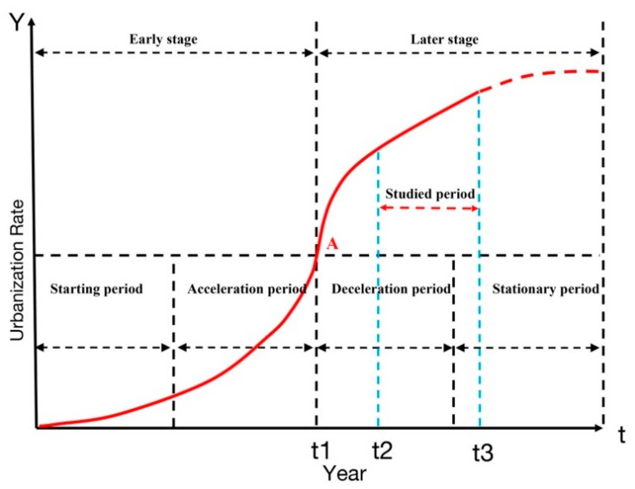
Figure 1. Urbanization stage regulation in different periods.
Sustainability 13 03661 g001
Figure 2. Factors’ changes during the studied period (1990–2019). (a) Urbanization rate changes; (b) Construction project investment changes during the studied period; (c) Real estate investment changes during the studied period; (d)Farmers’ investment changes during the studied period.
Sustainability 13 03661 g002
Figure 3. Proportion of different types of the total investment in fixed assets from 1990–2019.
Sustainability 13 03661 g003
Figure 4. Granger causality test results between urbanization rate and other indicators.
Sustainability 13 03661 g004
Figure 5. IRF response of Group ( l n U R , l n F I , l n C P I , and l n R E I ). (a) IRF response of l n U R to l n R E I ; (b) IRF response of l n U R to l n F I ; (c) IRF response of l n U R to l n C P I ; (d) IRF response of l n R E I to l n U R ; (e) IRF response of l n F I to l n U R ; (f) IRF response of l n C P I to l n U R .
Sustainability 13 03661 g005
Figure 6. IRF response of Group ( l n U R , l n T I ). (a) IRF response of l n T I   to   l n U R ; (b) IRF response of l n U R   to   l n T I .
Sustainability 13 03661 g006
Figure 7. Variance decomposition analysis of Group ( l n U R , l n T I ). (a) Variance decomposition analysis of percent l n U R variance due to l n U R ; (b) Variance decomposition analysis of percent l n U R variance due to l n T I .
Sustainability 13 03661 g007
Figure 8. Variance decomposition analysis of Group ( l n U R , l n F I , l n C P I , and l n R E I ). (a) Variance decomposition analysis of percent l n U R variance due to l n U R ; (b) Variance decomposition analysis of percent l n U R variance due to l n R E I ; (c) Variance decomposition analysis of percent l n U R variance due to l n F I ; (d) Variance decomposition analysis of percent l n U R variance due to l n C P I .
Sustainability 13 03661 g008
Figure 9. Results of Granger causality test, impulse response analysis and variance decomposition analysis.
Sustainability 13 03661 g009
Table 1. Results of the Jonhanse and Juselius co-integration test (Trace test and Maximum Eigenvalue test) between urbanization rate and other indicators at the 0.05 level.
Trace TestMaximum Eigenvalue Test
No. of CE(s)EigenvalueStatisticCritical ValueProb. **EigenvalueStatisticCritical ValueProb. **
LNUR and LNCPI, LNREI, LNFI
None *0.7678 59.0405 40.1749 0.0002 0.7678 37.9662 24.1592 0.0004
At most 10.3335 21.0744 24.2760 0.1202 0.3335 10.5505 17.7973 0.4289
At most 20.3078 10.5239 12.3209 0.0982 0.3078 9.5664 11.2248 0.0965
At most 30.0362 0.9575 4.1299 0.3799 0.0362 0.9575 4.1299 0.3799
LNUR and LNTI
None *0.5069 19.6435 12.3209 0.0025 0.5069 18.3839 11.2248 0.0024
At most 10.0473 1.2596 4.1299 0.3056 0.0473 1.2596 4.1299 0.3056
Max-eigenvalue test indicates 1 cointegrating eqn(s) at the 0.05 level. * denotes rejection of the hypothesis at the 0.05 level; ** MacKinnon-Haug-Michelis (1999) p-values.
Table 2. Optimal lag length test results between urbanization rate and other indicators.
LagLRFPEAICSCHQ
1/////
2 ( l n U R ,   l n F I ,   l n C P I   and   l n R E I )   and   ( l n U R ,   l n T I ) // ( l n U R ,   l n F I ,   l n C P I   and   l n R E I )   and   ( l n U R ,   l n T I )/
3/ ( l n U R ,   l n F I ,   l n C P I   and   l n R E I )   and   ( l n U R ,   l n T I )///
4// ( l n U R ,   l n F I ,   l n C P I   and   l n R E I )/ ( l n U R ,   l n F I ,   l n C P I   and   l n R E I )
5/////
6/////
7/////
8// ( l n U R ,   l n T I )/ ( l n U R ,   l n T I )
Publisher’s Note: MDPI stays neutral with regard to jurisdictional claims in published maps and institutional affiliations.