
Theoretical Comparison of the Effects of Different Traffic Conditions on Urban Road Environmental External Costs


Abstract
1. Introduction
1.1. Road Transport air Pollution Externality
1.2. Road Transport Climate Change Externality
1.3. Road Transport Noise Externality
1.4. Traffic Condition and Environmental Externalities
2. Methodology
- (1)
- Air pollution: , , , and are the considered air pollution-related environmental externalities.
- (2)
- Climate change: all emissions of GHG expressed in equivalents have been considered in the current paper.
- (3)
- Noise exposure: a distinction has been placed between six levels of persistent exposure: below 51 dB(A), 51–55 dB(A), 55–60 dB(A), 60–65 dB(A), 65–70 dB(A), and 70–75 dB(A) according to [1]. Each level is assessed with the corresponding health impacts.
2.1. Traffic Speed in Different Traffic Conditions: Monte Carlo Method
2.2. Air Pollutants and GHG Emission Estimation
- Exhaust emissions: are the emissions that are produced primarily from the combustion of different petroleum products which are mixtures of different hydrocarbons. Due to the imperfect combustion process, vehicle engines emit many different pollutants in addition to water and including , , , etc.The exhaust emissions would be further divided into “HOT” emissions when the engine is at its normal operating temperature, and “COLD-START” emissions, emissions during transient thermal engine operation.
- Abrasion emissions: are the emissions that are produced from the mechanical abrasion and corrosion of vehicle parts. Abrasion is only important for emissions and emissions of some heavy metals.
- Evaporative emissions: are the emissions from evaporating gasoline that contain a variety of different Hydrocarbons (), which can occur during vehicle refuelling, vehicle operation, and even when the vehicle is parked.
2.2.1. Emission Estimation
2.2.2. Emission Estimation
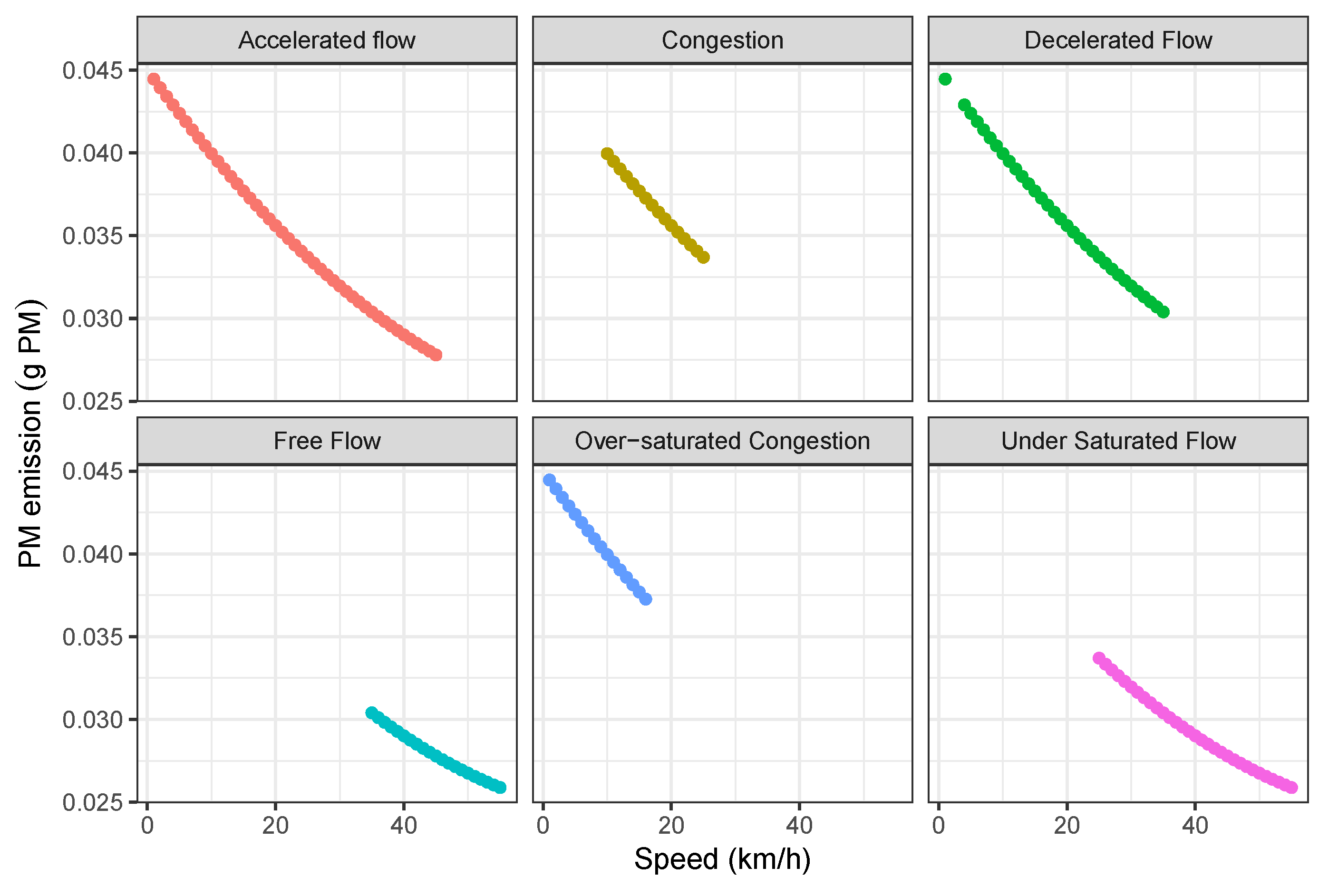
2.2.3. Emission Estimation
2.2.4. Emission Estimation
2.2.5. Emission Estimation
2.3. Noise Emission Estimation
2.4. Air Pollutants and GHG Cost Calculation
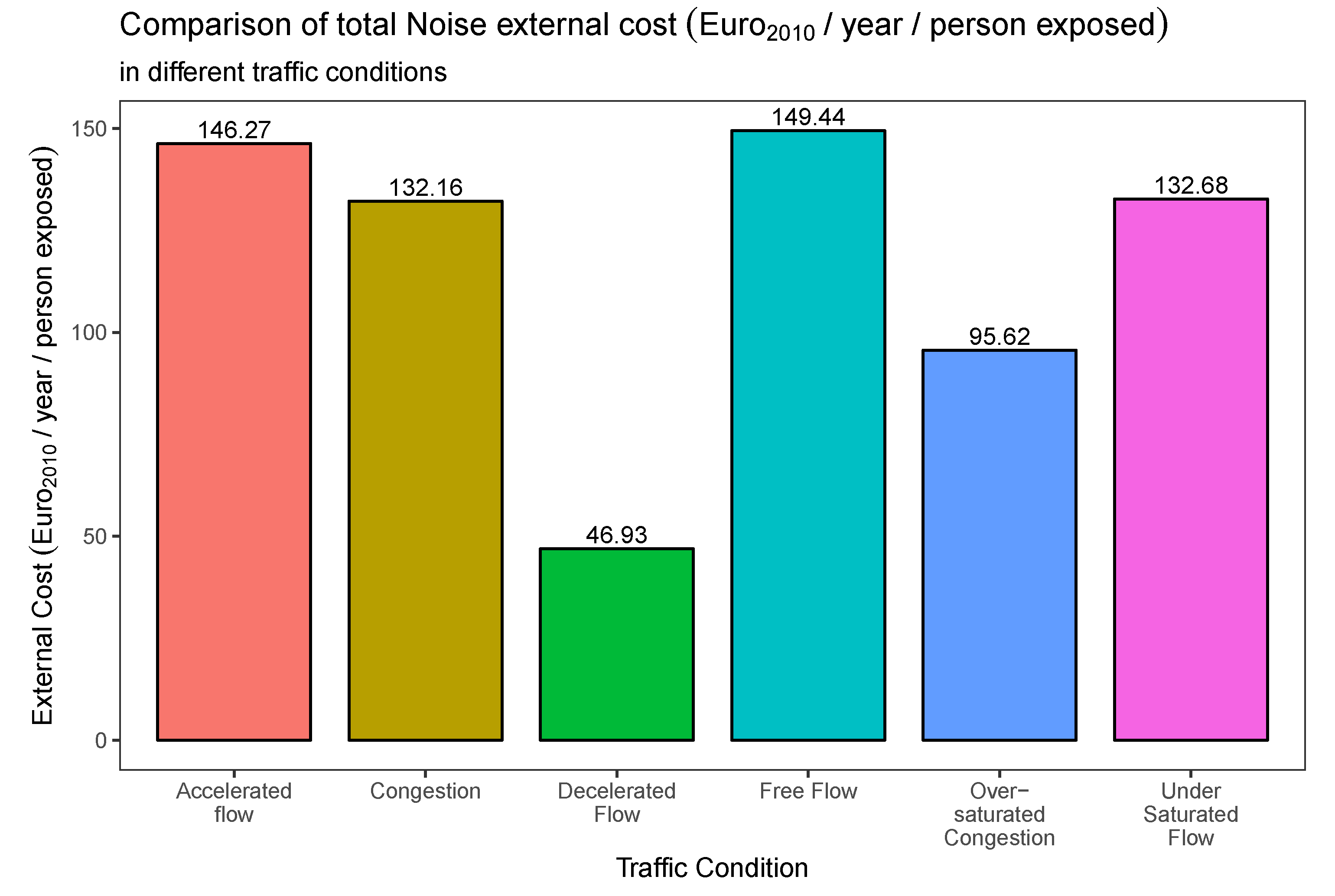
2.5. Noise Cost Calculation
3. Results
4. Discussion
5. Conclusions
Author Contributions
Funding
Data Availability Statement
Acknowledgments
Conflicts of Interest
References
- Korzhenevych, A.; Dehnen, N.; Bröcker, J.; Holtkamp, M.; Meier, H.; Gibson, G.; Varma, A.; Cox, V. Update of the Handbook on External Costs of Transport; Final Report for the European Commission, DG MOVE; MOVE. DIW Econ, CAU; Ricardo-AEA: London, UK, 2014. [Google Scholar]
- Santos, G. Road fuel taxes in Europe: Do they internalize road transport externalities? Transp. Policy 2017, 53, 120–134. [Google Scholar] [CrossRef]
- Santos, G.; Behrendt, H.; Maconi, L.; Shirvani, T.; Teytelboym, A. Part I: Externalities and economic policies in road transport. Res. Transp. Econ. 2010, 28, 2–45. [Google Scholar] [CrossRef]
- Pastorello, C.; Melios, G. Explaining Road Transport Emissions: A Non-Technical Guide; European Environment Agency: Luxembourg, 2016. [Google Scholar]
- Jochem, P.; Doll, C.; Fichtner, W. External costs of electric vehicles. Transp. Res. Part D Transp. Environ. 2016, 42, 60–76. [Google Scholar] [CrossRef]
- World Health Organization. Air Quality Guidelines: Global Update 2005; World Health Organization: Copenhagen, Denmark, 2006. [Google Scholar]
- Gehring, U.; Wijga, A.H.; Brauer, M.; Fischer, P.; de Jongste, J.C.; Kerkhof, M.; Oldenwening, M.; Smit, H.A.; Brunekreef, B. Traffic-related air pollution and the development of asthma and allergies during the first 8 years of life. Am. J. Respir. Crit. Care Med. 2010, 181, 596–603. [Google Scholar] [CrossRef] [PubMed]
- Jadaan, K.; Khreis, H.; Török, Á. Exposure to traffic-related air pollution and the onset of childhood asthma: A review of the literature and the assement methods used. Period. Polytech. Transp. Eng. 2018, 46, 21–28. [Google Scholar] [CrossRef]
- Amigou, A.; Sermage-Faure, C.; Orsi, L.; Leverger, G.; Baruchel, A.; Bertrand, Y.; Nelken, B.; Robert, A.; Michel, G.; Margueritte, G.; et al. Road traffic and childhood leukemia: The ESCALE study (SFCE). Environ. Health Perspect. 2010, 119, 566–572. [Google Scholar] [CrossRef]
- Fierro, M.A.; O’Rourke, M.K.; Burgess, J.L. Adverse Health Effects of Exposure to Ambient Carbon Monoxide; University of Arizona Report: Tucson, AZ, USA, 2001. [Google Scholar]
- Agency, E.E. Air Quality in Europe; Technical Report, EEA Technical Report No. 4/2012; European Environmental Agency (EEA): Copenhagen, Denmark, 2012. [Google Scholar]
- Perez, L.; Medina-Ramón, M.; Kunzli, N.; Alastuey, A.; Pey, J.; Pérez, N.; Garcia, R.; Tobías, A.; Querol, X.; Sunyer, J. Size fractionate particulate matter, vehicle traffic, and case-specific daily mortality in Barcelona, Spain. Environ. Sci. Technol. 2009, 43, 4707–4714. [Google Scholar] [CrossRef] [PubMed]
- Brauer, M.; Gehring, U.; Brunekreef, B.; de Jongste, J.; Gerritsen, J.; Rovers, M.; Wichmann, H.E.; Wijga, A.; Heinrich, J. Traffic-related air pollution and otitis media. Environ. Health Perspect. 2006, 114, 1414. [Google Scholar] [CrossRef] [PubMed]
- Buzási, A.; Csete, M.S. Ex-ante Assessment of Urban Development Projects. Eur. J. Sustain. Dev. 2017, 6, 267–267. [Google Scholar] [CrossRef][Green Version]
- Von Graevenitz, K. The amenity cost of road noise. J. Environ. Econ. Manag. 2018, 90, 1–22. [Google Scholar] [CrossRef]
- Sørensen, M.; Hvidberg, M.; Andersen, Z.J.; Nordsborg, R.B.; Lillelund, K.G.; Jakobsen, J.; Tjønneland, A.; Overvad, K.; Raaschou-Nielsen, O. Road traffic noise and stroke: A prospective cohort study. Eur. Heart J. 2011, 32, 737–744. [Google Scholar] [CrossRef]
- Sørensen, M.; Andersen, Z.J.; Nordsborg, R.B.; Becker, T.; Tjønneland, A.; Overvad, K.; Raaschou-Nielsen, O. Long-term exposure to road traffic noise and incident diabetes: A cohort study. Environ. Health Perspect. 2012, 121, 217–222. [Google Scholar] [CrossRef]
- Sørensen, M.; Andersen, Z.J.; Nordsborg, R.B.; Jensen, S.S.; Lillelund, K.G.; Beelen, R.; Schmidt, E.B.; Tjønneland, A.; Overvad, K.; Raaschou-Nielsen, O. Road traffic noise and incident myocardial infarction: A prospective cohort study. PLoS ONE 2012, 7, e39283. [Google Scholar] [CrossRef]
- World Health Organization. Burden of Disease from Environmental Noise: Quantification of Healthy Life Years Lost in Europe; World Health Organization, Regional Office for Europe: Copenhagen, Denmark, 2011. [Google Scholar]
- Barth, M.; Boriboonsomsin, K. Real-world carbon dioxide impacts of traffic congestion. Transp. Res. Rec. J. Transp. Res. Board 2008, 2058, 163–171. [Google Scholar] [CrossRef]
- Jacyna, M.; Wasiak, M.; Lewczuk, K.; Karoń, G. Noise and environmental pollution from transport: Decisive problems in developing ecologically efficient transport systems. J. Vibroeng. 2017, 19, 5639–5655. [Google Scholar] [CrossRef]
- Zhang, K.; Batterman, S. Air pollution and health risks due to vehicle traffic. Sci. Total Environ. 2013, 450, 307–316. [Google Scholar] [CrossRef] [PubMed]
- Gately, C.K.; Hutyra, L.R.; Peterson, S.; Wing, I.S. Urban emissions hotspots: Quantifying vehicle congestion and air pollution using mobile phone GPS data. Environ. Pollut. 2017, 229, 496–504. [Google Scholar] [CrossRef]
- Thaker, P.; Gokhale, S. The impact of traffic-flow patterns on air quality in urban street canyons. Environ. Pollut. 2016, 208, 161–169. [Google Scholar] [CrossRef] [PubMed]
- Zhong, N.; Cao, J.; Wang, Y. Traffic congestion, ambient air pollution, and health: Evidence from driving restrictions in Beijing. J. Assoc. Environ. Resour. Econ. 2017, 4, 821–856. [Google Scholar] [CrossRef]
- Lu, M.; Sun, C.; Zheng, S. Congestion and pollution consequences of driving-to-school trips: A case study in Beijing. Transp. Res. Part D Transp. Environ. 2017, 50, 280–291. [Google Scholar] [CrossRef]
- Wang, X.; Xue, Y.; Cen, B.l.; Zhang, P. Study on pollutant emissions of mixed traffic flow in cellular automaton. Phys. A Stat. Mech. Its Appl. 2020, 537, 122686. [Google Scholar] [CrossRef]
- Petro, F.; Konečnỳ, V. Calculation of Emissions from Transport Services and their use for the Internalisation of External Costs in Road Transport. Procedia Eng. 2017, 192, 677–682. [Google Scholar] [CrossRef]
- Jun, J. Understanding the variability of speed distributions under mixed traffic conditions caused by holiday traffic. Transp. Res. Part C Emerg. Technol. 2010, 18, 599–610. [Google Scholar] [CrossRef]
- Zou, Y.; Zhang, Y. Use of skew-normal and skew-t distributions for mixture modeling of freeway speed data. Transp. Res. Rec. J. Transp. Res. Board 2011, 2260, 67–75. [Google Scholar] [CrossRef]
- Wang, Y.; Dong, W.; Zhang, L.; Chin, D.; Papageorgiou, M.; Rose, G.; Young, W. Speed modeling and travel time estimation based on truncated normal and lognormal distributions. Transp. Res. Rec. J. Transp. Res. Board 2012, 2315, 66–72. [Google Scholar] [CrossRef]
- Wang, H.; Ni, D.; Chen, Q.Y.; Li, J. Stochastic Modeling of the Equilibrium Speed–Density Relationship. J. Adv. Transp. 2013, 47, 126–150. [Google Scholar] [CrossRef]
- Yu, R.; Abdel-Aty, M. An optimal variable speed limits system to ameliorate traffic safety risk. Transp. Res. Part C Emerg. Technol. 2014, 46, 235–246. [Google Scholar] [CrossRef]
- Maurya, A.; Dey, S.; Das, S. Speed and time headway distribution under mixed traffic condition. J. East. Asia Soc. Transp. Stud. 2015, 11, 1774–1792. [Google Scholar]
- Maghrour Zefreh, M.; Török, A. Distribution of traffic speed in different traffic conditions: An empirical study in Budapest. Transport 2020, 35, 68–86. [Google Scholar] [CrossRef]
- Kroese, D.P.; Brereton, T.; Taimre, T.; Botev, Z.I. Why the Monte Carlo method is so important today. Wiley Interdiscip. Rev. Comput. Stat. 2014, 6, 386–392. [Google Scholar] [CrossRef]
- Hu, Y.; Wang, F. Decomposing excess commuting: A Monte Carlo simulation approach. J. Transp. Geogr. 2015, 44, 43–52. [Google Scholar] [CrossRef]
- Gao, S.; Wang, Y.; Gao, Y.; Liu, Y. Understanding urban traffic-flow characteristics: A rethinking of betweenness centrality. Environ. Plan. B Plan. Des. 2013, 40, 135–153. [Google Scholar] [CrossRef]
- Wen, C.; Yang, C.; Pan, B.; Tian, Q. Traffic Efficiency of Ramp Intersection Based on Monte Carlo Simulation. In Proceedings of the CICTP 2020, Xi’an, China, 14–15 August 2020; pp. 265–276. [Google Scholar]
- Li, L.; Ji, X.; Gan, J.; Qu, X.; Ran, B. A Macroscopic Model of Heterogeneous Traffic Flow Based on the Safety Potential Field Theory. IEEE Access 2021, 9, 7460–7470. [Google Scholar] [CrossRef]
- Zambrano-Martinez, J.L.; Calafate, C.T.; Soler, D.; Cano, J.C.; Manzoni, P. Modeling and characterization of traffic flows in urban environments. Sensors 2018, 18, 2020. [Google Scholar] [CrossRef]
- Chrpa, L.; Magazzeni, D.; McCabe, K.; McCluskey, T.L.; Vallati, M. Automated planning for urban traffic control: Strategic vehicle routing to respect air quality limitations. Intell. Artif. 2016, 10, 113–128. [Google Scholar] [CrossRef]
- Jandacka, D.; Durcanska, D.; Bujdos, M. The contribution of road traffic to particulate matter and metals in air pollution in the vicinity of an urban road. Transp. Res. Part D Transp. Environ. 2017, 50, 397–408. [Google Scholar] [CrossRef]
- Rodríguez, M.C.; Dupont-Courtade, L.; Oueslati, W. Air pollution and urban structure linkages: Evidence from European cities. Renew. Sustain. Energy Rev. 2016, 53, 1–9. [Google Scholar] [CrossRef]
- Sun, C.; Luo, Y.; Li, J. Urban traffic infrastructure investment and air pollution: Evidence from the 83 cities in China. J. Clean. Prod. 2018, 172, 488–496. [Google Scholar] [CrossRef]
- e Almeida, L.d.O.; Favaro, A.; Raimundo-Costa, W.; Anhê, A.C.B.M.; Ferreira, D.C.; Blanes-Vidal, V.; dos Santos Senhuk, A.P.M. Influence of urban forest on traffic air pollution and children respiratory health. Environ. Monit. Assess. 2020, 192, 1–9. [Google Scholar] [CrossRef]
- Smith, L.; Mukerjee, S.; Kovalcik, K.; Sams, E.; Stallings, C.; Hudgens, E.; Scott, J.; Krantz, T.; Neas, L. Near-road measurements for nitrogen dioxide and its association with traffic exposure zones. Atmos. Pollut. Res. 2015, 6, 1082–1086. [Google Scholar] [CrossRef]
- Yamada, H.; Hayashi, R.; Tonokura, K. Simultaneous measurements of on-road/in-vehicle nanoparticles and NOx while driving: Actual situations, passenger exposure and secondary formations. Sci. Total Environ. 2016, 563, 944–955. [Google Scholar] [CrossRef]
- EEAE. EEA Air Pollutant Emission Inventory Guidebook—2009; European Environment Agency (EEA): Copenhagen, Denmark, 2009. [Google Scholar]
- Joumard, R.; Sérié, E. Modelling of cold start emissions for passenger cars. Inrets Rep. LTE 1999, 9931, 86. [Google Scholar]
- EUCO. Conclusions European Council 4 February 2011. Conclusions EUCO 2/1/1(REV 1): 1-15; Technical Report; EUROPEAN COUNCIL: Brussels, Belgium, 2011. [Google Scholar]
- Fuzzi, S.; Baltensperger, U.; Carslaw, K.; Decesari, S.; Van Der Gon, H.D.; Facchini, M.; Fowler, D.; Koren, I.; Langford, B.; Lohmann, U.; et al. Particulate matter, air quality and climate: Lessons learned and future needs. Atmos. Chem. Phys. 2015, 15, 8217–8299. [Google Scholar] [CrossRef]
- Monks, P.S.; Archibald, A.; Colette, A.; Cooper, O.; Coyle, M.; Derwent, R.; Fowler, D.; Granier, C.; Law, K.S.; Mills, G.; et al. Tropospheric ozone and its precursors from the urban to the global scale from air quality to short-lived climate forcer. Atmos. Chem. Phys. 2015, 15, 8889–8973. [Google Scholar] [CrossRef]
- Cox, L.; Blaszczak, R. Nitrogen Oxides (NOx) Why and How They Are Controlled; DIANE Publishing: Darby, PA, USA, 1999. [Google Scholar]
- Mills, I.C.; Atkinson, R.W.; Kang, S.; Walton, H.; Anderson, H. Quantitative systematic review of the associations between short-term exposure to nitrogen dioxide and mortality and hospital admissions. BMJ Open 2015, 5, e006946. [Google Scholar] [CrossRef] [PubMed]
- Englert, N. Fine particles and human health—a review of epidemiological studies. Toxicol. Lett. 2004, 149, 235–242. [Google Scholar] [CrossRef]
- Michaels, R.A.; Kleinman, M.T. Incidence and apparent health significance of brief airborne particle excursions. Aerosol Sci. Technol. 2000, 32, 93–105. [Google Scholar] [CrossRef]
- Bell, M.L.; Ebisu, K.; Leaderer, B.P.; Gent, J.F.; Lee, H.J.; Koutrakis, P.; Wang, Y.; Dominici, F.; Peng, R.D. Associations of PM2. 5 constituents and sources with hospital admissions: Analysis of four counties in Connecticut and Massachusetts (USA) for persons≥ 65 years of age. Environ. Health Perspect. 2013, 122, 138–144. [Google Scholar] [CrossRef]
- Kheirbek, I.; Haney, J.; Douglas, S.; Ito, K.; Matte, T. The contribution of motor vehicle emissions to ambient fine particulate matter public health impacts in New York City: A health burden assessment. Environ. Health 2016, 15, 89. [Google Scholar] [CrossRef]
- Heydari, S.; Tainio, M.; Woodcock, J.; de Nazelle, A. Estimating traffic contribution to particulate matter concentration in urban areas using a multilevel Bayesian meta-regression approach. Environ. Int. 2020, 141, 105800. [Google Scholar] [CrossRef] [PubMed]
- Gao, H.O. Particulate matter exposure at a densely populated urban traffic intersection and crosswalk. Environ. Pollut. 2020, 268, 115931. [Google Scholar]
- Chalermpong, S.; Thaithatkul, P.; Anuchitchanchai, O.; Sanghatawatana, P. Land use regression modeling for fine particulate matters in Bangkok, Thailand, using time-variant predictors: Effects of seasonal factors, open biomass burning, and traffic-related factors. Atmos. Environ. 2020, 246, 118128. [Google Scholar] [CrossRef]
- Yang, M.; Ma, T.; Sun, C. Evaluating the impact of urban traffic investment on SO 2 emissions in China cities. Energy Policy 2018, 113, 20–27. [Google Scholar] [CrossRef]
- Guttikunda, S.K.; Carmichael, G.R.; Calori, G.; Eck, C.; Woo, J.H. The contribution of megacities to regional sulfur pollution in Asia. Atmos. Environ. 2003, 37, 11–22. [Google Scholar] [CrossRef]
- Chen, X.; Shao, S.; Tian, Z.; Xie, Z.; Yin, P. Impacts of air pollution and its spatial spillover effect on public health based on China’s big data sample. J. Clean. Prod. 2017, 142, 915–925. [Google Scholar] [CrossRef]
- Guarnaccia, C. Advanced tools for traffic noise modelling and prediction. WSEAS Trans. Syst. 2013, 12, 121–130. [Google Scholar]
- Hansell, A.L.; Blangiardo, M.; Fortunato, L.; Floud, S.; de Hoogh, K.; Fecht, D.; Ghosh, R.E.; Laszlo, H.E.; Pearson, C.; Beale, L.; et al. Aircraft noise and cardiovascular disease near Heathrow airport in London: Small area study. BMJ 2013, 347, f5432. [Google Scholar] [CrossRef]
- Hammer, M.S.; Swinburn, T.K.; Neitzel, R.L. Environmental noise pollution in the United States: Developing an effective public health response. Environ. Health Perspect. 2014, 122, 115. [Google Scholar] [CrossRef]
- WHO. Night noise guidelines for Europe; World Health Organization-Regional Office for Europe: Copenhagen, Denmark, 2009. [Google Scholar]
- Babisch, W.; Pershagen, G.; Selander, J.; Houthuijs, D.; Breugelmans, O.; Cadum, E.; Vigna-Taglianti, F.; Katsouyanni, K.; Haralabidis, A.S.; Dimakopoulou, K.; et al. Noise annoyance—A modifier of the association between noise level and cardiovascular health? Sci. Total Environ. 2013, 452, 50–57. [Google Scholar] [CrossRef]
- Clark, C.; Crombie, R.; Head, J.; Van Kamp, I.; Van Kempen, E.; Stansfeld, S.A. Does traffic-related air pollution explain associations of aircraft and road traffic noise exposure on children’s health and cognition? A secondary analysis of the United Kingdom sample from the RANCH project. Am. J. Epidemiol. 2012, 176, 327–337. [Google Scholar] [CrossRef]
- Clark, C.; Head, J.; Stansfeld, S.A. Longitudinal effects of aircraft noise exposure on children’s health and cognition: A six-year follow-up of the UK RANCH cohort. J. Environ. Psychol. 2013, 35, 1–9. [Google Scholar] [CrossRef]
- Maghrour Zefreh, M.; Torok, A. Theoretical Comparison of the Effects of Different Traffic Conditions on Urban Road Traffic Noise. J. Adv. Transp. 2018, 2018, 7949574. [Google Scholar] [CrossRef]
- Gulliver, J.; Morley, D.; Vienneau, D.; Fabbri, F.; Bell, M.; Goodman, P.; Beevers, S.; Dajnak, D.; J Kelly, F.; Fecht, D. Development of an Open-Source Road Traffic Noise Model for Exposure Assessment. Environ. Model. Softw. 2015, 74, 183–193. [Google Scholar] [CrossRef]
- Barry, T.M.; Reagan, J.A. FHWA Highway Traffic Noise Prediction Model, FHWA-RD-77-108; US Department of Transportation, Federal Highway Administration, Office of Environmental Policy: Washington, DC, USA, 1978.
- Department of Transport, Welsh Office. Calculation of Road Traffic Noise; HMSO Publication: London, England, UK, 1988. [Google Scholar]
- Quartieri, J.; Mastorakis, N.; Iannone, G.; Guarnaccia, C.; D’ambrosio, S.; Troisi, A.; Lenza, T. A review of traffic noise predictive models. In Recent Advances in Applied and Theoretical Mechanics. In Proceedings of the 5th WSEAS International Conference on Applied and Theoretical Mechanics (MECHANICS’09) Puerto De La Cruz, Tenerife, Canary Islands, Spain, 14–16 December 2009; pp. 14–16. [Google Scholar]
- Sakamoto, S. Road Traffic Noise Prediction Model“ASJ RTN-Model 2013”: Report of the Research Committee on Road Traffic Noise. Acoust. Sci. Technol. 2015, 36, 49–108. [Google Scholar] [CrossRef]
- Watts, G. Harmonoise Prediction Model for Road Traffic Noise; TRL published project report PPR 034; TRL: Wokingham, UK, 2005. [Google Scholar]
- Heutschi, K. SonRoad: New Swiss road traffic noise model. Acta Acust. United Acust. 2004, 90, 548–554. [Google Scholar]
- Kragh, J.; Plovsing, B.; Storeheier, S.; Jonasson, H. Nordic Environmental Noise Prediction Methods, Nord2000 Summary Report; DELTA Danish Electronics, Light, & Acoustics: Lyngby, Denmark, 2002. [Google Scholar]
- Dutilleux, G.; Defrance, J.; Ecotière, D.; Gauvreau, B.; Bérengier, M.; Besnard, F.; Duc, E.L. NMPB-ROUTES-2008: The revision of the French method for road traffic noise prediction. Acta Acust. United Acust. 2010, 96, 452–462. [Google Scholar] [CrossRef]
- Garg, N.; Maji, S. A critical review of principal traffic noise models: Strategies and implications. Environ. Impact Assess. Rev. 2014, 46, 68–81. [Google Scholar] [CrossRef]
- Directive, E. Directive 2002/49/EC of the European parliament and the Council of 25 June 2002 relating to the assessment and management of environmental noise. Off. J. Eur. Communities 2002, 189, 2002. [Google Scholar]
- Mashayekh, Y.; Jaramillo, P.; Chester, M.; Hendrickson, C.; Weber, C. Costs of automobile air emissions in US metropolitan areas. Transp. Res. Rec. J. Transp. Res. Board 2011, 2233, 120–127. [Google Scholar] [CrossRef]
- Bank of England: Spot Exchange Rate. Available online: https://www.poundsterlinglive.com/bank-of-england-spot/historical-spot-exchange-rates/usd/USD-to-EUR-2007 (accessed on 30 November 2018).
- Eurostat. Available online: https://ec.europa.eu/eurostat/tgm/refreshTableAction.do?tab=table&plugin=1&pcode=sdg_08_10&language=en (accessed on 30 November 2018).
- Maibach, M.; Schreyer, C.; Sutter, D.; Van Essen, H.; Boon, B.; Smokers, R.; Schroten, A.; Doll, C.; Pawlowska, B.; Bak, M. Handbook on estimation of external costs in the transport sector. Ce Delft 2008. version 1.1, 2. [Google Scholar]
- Weinmayr, G.; Hennig, F.; Fuks, K.; Nonnemacher, M.; Jakobs, H.; Möhlenkamp, S.; Erbel, R.; Jöckel, K.H.; Hoffmann, B.; Moebus, S. Long-term exposure to fine particulate matter and incidence of type 2 diabetes mellitus in a cohort study: Effects of total and traffic-specific air pollution. Environ. Health 2015, 14, 53. [Google Scholar] [CrossRef] [PubMed]
- Adom, P.K.; Kwakwa, P.A.; Amankwaa, A. The long-run effects of economic, demographic, and political indices on actual and potential CO2 emissions. J. Environ. Manag. 2018, 218, 516–526. [Google Scholar] [CrossRef] [PubMed]
- Lin, B.; Xu, M. Regional differences on CO2 emission efficiency in metallurgical industry of China. Energy Policy 2018, 120, 302–311. [Google Scholar] [CrossRef]
- Andersson, F.N.; Opper, S.; Khalid, U. Are capitalists green? Firm ownership and provincial CO2 emissions in China. Energy Policy 2018, 123, 349–359. [Google Scholar] [CrossRef]
- Lo, P.L.; Martini, G.; Porta, F.; Scotti, D. The determinants of CO2 emissions of air transport passenger traffic: An analysis of Lombardy (Italy). Transp. Policy 2020, 91, 108–119. [Google Scholar] [CrossRef]


| Traffic Condition | Fitted Speed Distribution | Minimum Speed (km/h) | Maximum Speed (km/h) | Average Speed (km/h) | Standard Deviation of Speed (km/h) |
|---|---|---|---|---|---|
| Free flow | Log-normal distribution | 35 | 55 | 47.18 | 5.5 |
| Accelerated flow | Beta distribution | 1 | 45 | 27.41 | 13.15 |
| Over-saturated congestion | Exponential distribution | 1 | 15.5 | 10.37 | 2.74 |
| Undersaturated flow | Normal distribution | 25 | 55 | 38.14 | 6.46 |
| Decelerated flow | Chi-square distribution | 1 | 35 | 18.76 | 11.82 |
| Congestion | Gamma distribution | 10 | 25 | 14.53 | 3.91 |
| # Vehicles | Vehicle Type | Engine Type | Engine Size | Road Length |
|---|---|---|---|---|
| 1600 passenger car | Euro IV | Diesel engine | <2.0 | 1 km of urban road |
| Air Pollutant/GHG | |||||
|---|---|---|---|---|---|
| (Urban Area) | |||||
| EU average cost | 270178 | 10640 | 10241 | 90 | 497.8 |
| (dB(A)) | ||||||
|---|---|---|---|---|---|---|
| 51 | 55 | 60 | 65 | 70 | 75 | |
| EU average cost | 8.28 | 41.04 | 82.32 | 123.24 | 164.48 | 273.36 |
| Traffic Condition | Air Pollutants and GHG Cost €(2010) | Noise Cost €(2010)/ Year/Person Exposed Noise | |||||
|---|---|---|---|---|---|---|---|
| Total | |||||||
| Free flow | 21.12 | 8.63 | 12.09 | 0.06 | 0.06 | 41.97 | 149.44 |
| Under sat. flow | 22.22 | 9.50 | 12.78 | 0.07 | 0.07 | 44.63 | 132.68 |
| compared to free flow | 5.19% | 10% | 5.68% | 5.19% | 25.88% | 6% | −11% |
| Congestion | 32.23 | 14.28 | 16.28 | 0.10 | 0.18 | 63.06 | 132.16 |
| compared to free flow | 52.59% | 65.41% | 34.63% | 52.59% | 208.94% | 50% | −12% |
| Over-sat. congestion | 46.18 | 16.65 | 17.92 | 0.14 | 0.26 | 81.15 | 95.62 |
| compared to free flow | 118.64% | 92.88% | 48.21% | 118.64% | 339.99% | 93% | −36% |
| Accelerated flow | 28.36 | 11.90 | 14.53 | 0.08 | 0.13 | 55.01 | 146.27 |
| compared to free flow | 34.26% | 37.86% | 20.22% | 34.26% | 121.85% | 31% | −2% |
| Decelerated flow | 30.69 | 13.65 | 15.83 | 0.09 | 0.16 | 60.42 | 46.93 |
| compared to free flow | 45.29% | 58.10% | 30.91% | 45.29% | 182.17% | 44% | −69% |
Publisher’s Note: MDPI stays neutral with regard to jurisdictional claims in published maps and institutional affiliations. |
© 2021 by the authors. Licensee MDPI, Basel, Switzerland. This article is an open access article distributed under the terms and conditions of the Creative Commons Attribution (CC BY) license (http://creativecommons.org/licenses/by/4.0/).
Share and Cite
Zefreh, M.M.; Torok, A. Theoretical Comparison of the Effects of Different Traffic Conditions on Urban Road Environmental External Costs. Sustainability 2021, 13, 3541. https://doi.org/10.3390/su13063541
Zefreh MM, Torok A. Theoretical Comparison of the Effects of Different Traffic Conditions on Urban Road Environmental External Costs. Sustainability. 2021; 13(6):3541. https://doi.org/10.3390/su13063541
Chicago/Turabian StyleZefreh, Mohammad Maghrour, and Adam Torok. 2021. "Theoretical Comparison of the Effects of Different Traffic Conditions on Urban Road Environmental External Costs" Sustainability 13, no. 6: 3541. https://doi.org/10.3390/su13063541
APA StyleZefreh, M. M., & Torok, A. (2021). Theoretical Comparison of the Effects of Different Traffic Conditions on Urban Road Environmental External Costs. Sustainability, 13(6), 3541. https://doi.org/10.3390/su13063541