
Local Dynamic Path Planning for an Ambulance Based on Driving Risk and Attraction Field


Abstract
1. Introduction
2. Literature Review
2.1. Ambulance Planning
2.2. Potential Field for Path Planning
3. Potential Field Modelling
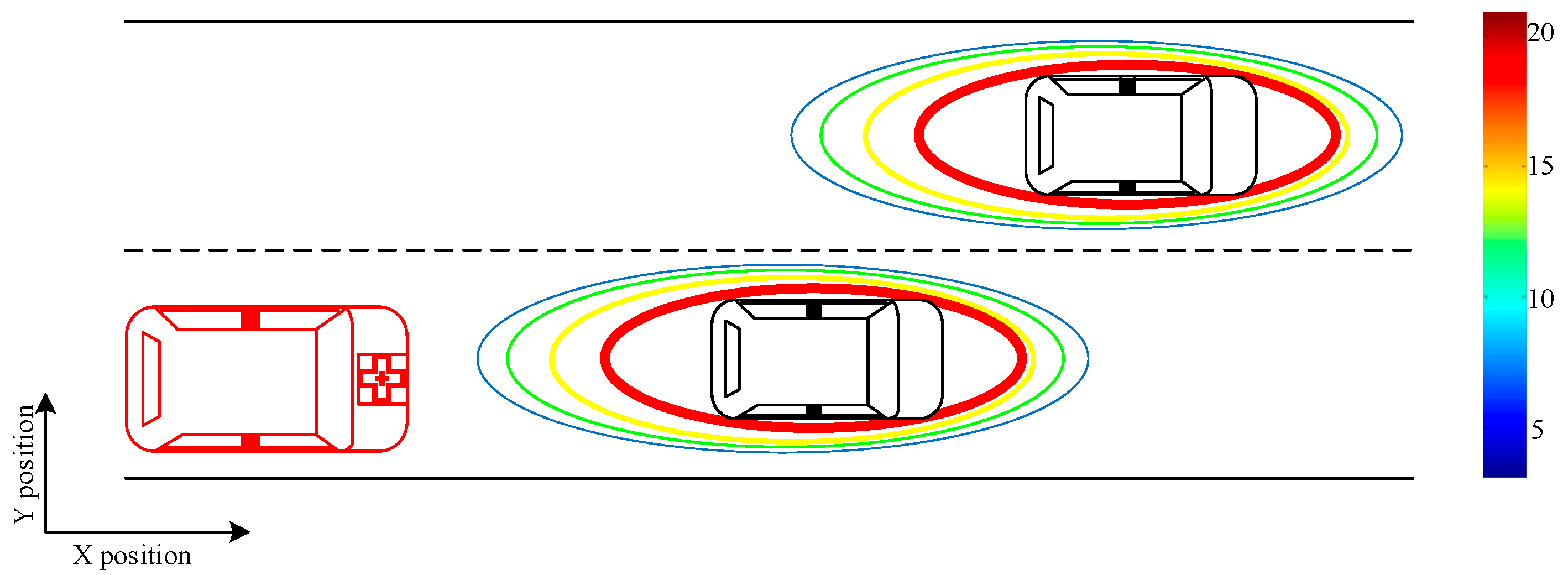
3.1. Repulsive PF Model
- Road Boundary Potential Field
- Lane Line Potential Field
- Obstacle Potential Field
3.2. Attractive PF Model
- Target Potential Field
- Lane Velocity Potential
- Tailgating Potential
4. Simulation Construction
4.1. Simulation and Parameter Design
4.2. Results Discussion
4.2.1. Simulation Result
4.2.2. Results Comparison
5. Conclusions
Author Contributions
Funding
Conflicts of Interest
References
- Akıncılar, A.; Akıncılar, E. A new idea for ambulance location problem in an environment under uncertainty in both path and average speed: Absolutely robust planning. Comput. Indus. Eng. 2019, 137, 106053. [Google Scholar] [CrossRef]
- O’Keeffe, C.; Nicholl, J.; Turner, J.; Goodacre, S. Role of ambulance response times in the survival of patients with out-of-hospital cardiac arrest. Emerg. Med. J. 2011, 28, 703–706. [Google Scholar] [CrossRef]
- Kergosien, Y.B. A Generic and Flexible Simulation-Based Analysis Tool for EMS Management. Int. J. Prod. Res. 2015, 53, 7299–7316. [Google Scholar] [CrossRef]
- Rokos, I.; Henry, T.; Weittenhiller, B.; Bjerke, C.; Bates, E.; French, W. Mission: Lifeline STEMI Networks Geospatial Information Systems (GIS) Maps. Crit. Pathw. Cardiol. 2013, 12, 43–44. [Google Scholar] [CrossRef] [PubMed]
- Roessler, M. EMS systems in Germany. Resuscitation 2006, 68, 45–49. [Google Scholar] [CrossRef] [PubMed]
- Montemerlo, M.; Becker, J.; Bhat, S.; Dahlkamp, H.; Thrun, S. Junior: The Stanford entry in the Urban Challenge. J. Field Robot. 2008, 25, 569–597. [Google Scholar] [CrossRef]
- Dolgov, D.; Thrun, S.; Montemerlo, M.; Diebel, J. Path Planning for Autonomous Vehicles in Unknown Semi-structured Environments. Int. J. Robot. Res. 2010, 29, 485–501. [Google Scholar] [CrossRef]
- Chu, K.; Kim, J.; Jo, K.; Sunwoo, M. Real-time path planning of autonomous vehicles for unstructured road navigation. Int. J. Auto. Tech. 2015, 16, 653–668. [Google Scholar] [CrossRef]
- Karaman, S.; Frazzoli, E. Sampling-based algorithms for optimal motion planning. Int. J. Robot. Res. 2011, 30, 846–894. [Google Scholar] [CrossRef]
- Khatib, O. Real-Time Obstacle Avoidance for Manipulators and Mobile Robots. In Proceedings of the 1985 IEEE International Conference on Robotics and Automation, St. Louis, MO, USA, 25–28 March 1985. [Google Scholar]
- Rasekhipour, Y.; Khajepour, A.; Chen, S.K.; Litkouh, B. A Potential Field-Based Model Predictive Path-Planning Controller for Autonomous Road Vehicles. IEEE Trans. Intell. Transp. Syst. 2017, 18, 1255–1267. [Google Scholar] [CrossRef]
- Tu, Q.; Chen, H.; Li, J. A Potential Field Based Lateral Planning Method for Autonomous Vehicles. SAE Int. J. Passeng. Cars Electron. Electr. Syst. 2017, 10, 24–34. [Google Scholar] [CrossRef]
- Wahid, N.; Zamzuri, H.; Rahman, M.A.A.; Kuroda, S.; Raksincharoensak, P. Study on potential field based motion planning and control for automated vehicle collision avoidance systems. In Proceedings of the IEEE International Conference on Mechatronics, Churchill, VIC, Australia, 13–15 February 2017; IEEE: Victoria, Australia, 2017; pp. 208–213. [Google Scholar]
- Wu, B.; Yan, Y.; Ni, D.H.; Li, L.B. A longitudinal car-following risk assessment model based on risk field theory for autonomous vehicles. Int. J. Transport. Sci. Tech. 2020. [Google Scholar] [CrossRef]
- Noto, N.; Okuda, H.; Tazaki, Y. Steering assisting system for obstacle avoidance based on personalized potential field. In Proceedings of the IEEE 15th ITSC, Anchorage, AK, USA, 16–19 September 2012; pp. 1702–1707. [Google Scholar]
- Akincilar, A.; Akincilar, E. A specific issue on sustainability of transportation planning in an urban region: Ambulance location problem. In Sustainable Infrastructure; IGI Global: Hershey, PA, USA, 2017; pp. 303–310. [Google Scholar]
- Basar, A.; Catay, B.; Unluyurt, T. A taxonomy for emergency service station location problem. Optim. Lett. 2012, 6, 1147–1160. [Google Scholar] [CrossRef]
- Campbell, A.M.; Vandenbussche, D.; Hermann, W. Routing for relief efforts. Transp. Sci. 2008, 42, 127–145. [Google Scholar] [CrossRef]
- Henderson, S.G.; Lewis, M.E. Two-class routing with admission control and strict priorities. Prob. Eng. Inform. Sci. 2018, 32, 163–178. [Google Scholar]
- Nordin, N.A. An application of the A* algorithm on the ambulance routing. In Proceedings of the 2011 IEEE Colloquium on Humanities, Science and Engineering, Penang, Malaysia, 5–6 December 2011; pp. 855–859. [Google Scholar]
- Panahi, S. Dynamic shortest path in ambulance routing based on GIS. Int. J. Geo. 2009, 5, 13–19. [Google Scholar]
- Patel, A.; Waters, N. Using Geographic Information Systems for Health Research. In Application of Geographic Information System; InTech: Edmonton, AB, Canada, 2012. [Google Scholar]
- ReVelle, C.; Bigman, D.; Schilling, D.; Cohon, J.; Church, R. Facility location: A review of context-free and EMS models. Health Serv. Res. 1977, 12, 129–146. [Google Scholar] [PubMed]
- Erkut, E.; Ingolfsson, A.; Erdogan, G. Ambulance location for maximum survival. Nav. Res. Logist. 2008, 55, 42–58. [Google Scholar] [CrossRef]
- Chanta, S.; Mayorga, M.E.; Kurz, M.E.; McLay, L.A. The minimum p-envy location problem: A new model for equitable distribution of emergency resources. IIE Trans. Healthc. Syst. Eng. 2011, 1, 101–115. [Google Scholar] [CrossRef]
- Drezner, T.; Drezner, Z.; Guyse, J. Equitable service by a facility: Minimizing the Gini coefficient. Comput. Oper. Res. 2009, 36, 3240–3246. [Google Scholar] [CrossRef]
- Espejo, I.; Marin, A.; Puerto, J.; Rodriguez-Chia, A.M. A comparison of formulations and solution methods for the minimum-envy location problem. Comput. Oper. Res. 2009, 36, 1966–1981. [Google Scholar] [CrossRef]
- Chanta, S.; Mayorga, M.E.; McLay, L.A. Improving emergency service in rural areas: A bi-objective covering location model for EMS systems. Ann. Oper. Res. 2014, 221, 133–159. [Google Scholar] [CrossRef]
- Khodaparasti, S.; Maleki, H.R.; Bruni, M.E.; Jahedi, S.; Beraldi, P.; Conforti, D. Balancing efficiency and equity in location-allocation models with an application to strategic EMS design. Optim. Lett. 2016, 10, 1053–1070. [Google Scholar] [CrossRef]
- Tang, J.; Chen, X.; Hu, Z.; Zong, F.; Han, C.Y.; Li, L.X. Traffic flow prediction based on combination of support vector machine and data denoising schemes. Phys. A Stat. Mech. Its Appl. 2019, 534. [Google Scholar] [CrossRef]
- Brotcorne, L.; Laporte, G.; Semet, F. Ambulance location and relocation models. Eur. J. Oper. Res. 2003, 147, 451–463. [Google Scholar] [CrossRef]
- Gendreau, M.; Laporte, G.; Semet, F. A dynamic model and parallel tabu search heuristic for real-time ambulance relocation. Par. Comput. 2001, 27, 1641–1653. [Google Scholar] [CrossRef]
- Berman, O.; Hajizadeh, I.; Krass, D. The maximum covering problem with travel time uncertainty. IIE Trans. 2013, 45, 81–96. [Google Scholar] [CrossRef]
- Schmid, V.; Doerner, K.F. Ambulance location and relocation problems with time-dependent travel times. Eur. J. Oper. Res. 2010, 207, 1293–1303. [Google Scholar] [CrossRef]
- Schmid, V. Solving the dynamic ambulance relocation and dispatching problem using approximate dynamic programming. Eur. J. Oper. Res. 2012, 219, 611. [Google Scholar] [CrossRef]
- Tlili, T.; Harzi, M.; Krichen, S. Swarm-based approach for solving the ambulance routing problem. Proc. Comput. Sci. 2017, 112, 350–357. [Google Scholar] [CrossRef]
- Yoon, S.; Albert, L.A. A dynamic ambulance routing model with multiple response. Transp. Res. Part E Logist. Transp. Rev. 2020, 133, 101807. [Google Scholar] [CrossRef]
- Gayathri, N. A novel technique for optimal vehicle routing. In Proceedings of the 2014 International Conference on Electronics and Communication Systems (ICECS), Coimbatore, India, 13–14 February 2014; pp. 1–5. [Google Scholar]
- Maxwell, M.S. Approximate dynamic programming for ambulance redeployment. INFORMS J. Comput. 2010, 22, 266–281. [Google Scholar] [CrossRef]
- Cao, Z.G.; Guo, H.L.; Zhang, J.; Niyato, D. Finding the Shortest Path in Stochastic Vehicle Routing: A Cardinality Minimization Approach. IEEE Trans. Intell. Transp. Syst. 2016, 17, 1688–1702. [Google Scholar] [CrossRef]
- Cao, Z.G.; Guo, H.L.; Song, W.; Gao, K.Z.; Chen, Z.H.; Zhang, L.; Zhang, X.X. Using Reinforcement Learning to Minimize the Probability of Delay Occurrence in Transportation. IEEE Trans. Veh. Tech. 2020, 69, 2424–2436. [Google Scholar] [CrossRef]
- Cao, Z.G.; Guo, H.L.; Zhang, J.; Niyato, D.; Fastenrath, U. Improving the Efficiency of Stochastic Vehicle Routing: A Partial Lagrange Multiplier Method. IEEE Trans. Veh. Tech. 2016, 65, 3933–4005. [Google Scholar] [CrossRef]
- Raja, R.; Dutta, A.; Venkatesh, K. New potential field method for rough terrain path planning using genetic algorithm for a 6-wheel rover. Robot. Auto. Syst. 2015, 72, 295–306. [Google Scholar] [CrossRef]
- Matoui, F.; Boussaid, B.; Abdelkrim, M.N. Local minimum solution for the potential field method in multiple robot motion planning task. In Proceedings of the 2015 16th International Conference on Sciences and Techniques of Automatic Control and Computer Engineering (STA), Monastir, Tunisia, 21–23 December 2016; pp. 452–457. [Google Scholar]
- Ruan, Y.; Chen, H.; Li, J. Longitudinal Planning and Control Method for Autonomous Vehicles Based on A New Potential Field Model. SAE Tech. Pap. 2017. [Google Scholar] [CrossRef]
- Hu, H.; Zhang, C.; Sheng, Y.; Zhou, B.; Gao, F. An improved artificial potential field model considering vehicle velocity for autonomous driving. IFAC 2018, 51, 863–867. [Google Scholar]
- Zong, F.; Zeng, M.; He, Z.; Yuan, Y. Bus-Car Mode Identification: Traffic Condition–Based Random-Forests Method. J. Transp. Eng. Part A Syst. 2020, 146, 04020113. [Google Scholar] [CrossRef]
- Wang, J.; Wu, J.; Li, Y. The driving safety field based on driver–vehicle–road interactions. IEEE Trans. Intell. Transp. Syst. 2015, 16, 2203–2214. [Google Scholar] [CrossRef]


| Potential | Object | Parameter | Definition | Value |
|---|---|---|---|---|
| Repulsive potential | Road boundary | Coefficient of road boundary potential | 20.00 | |
| Lane line | Coefficient of lane line potential | 1.00 | ||
| Obstacle | Coefficient of obstacle potential | 10.00 | ||
| Convergence coefficient in x direction | 10.00 | |||
| Convergence coefficient in y direction | 1.50 | |||
| Attractive potential | Target | Coefficient of target potential | 0.25 | |
| Lane velocity | Coefficient of lane-velocity potential | 0.14 | ||
| Tailgating | Coefficient of tailgating potential | 10.00 |
| Item | Max | Min | Variance | Mean |
|---|---|---|---|---|
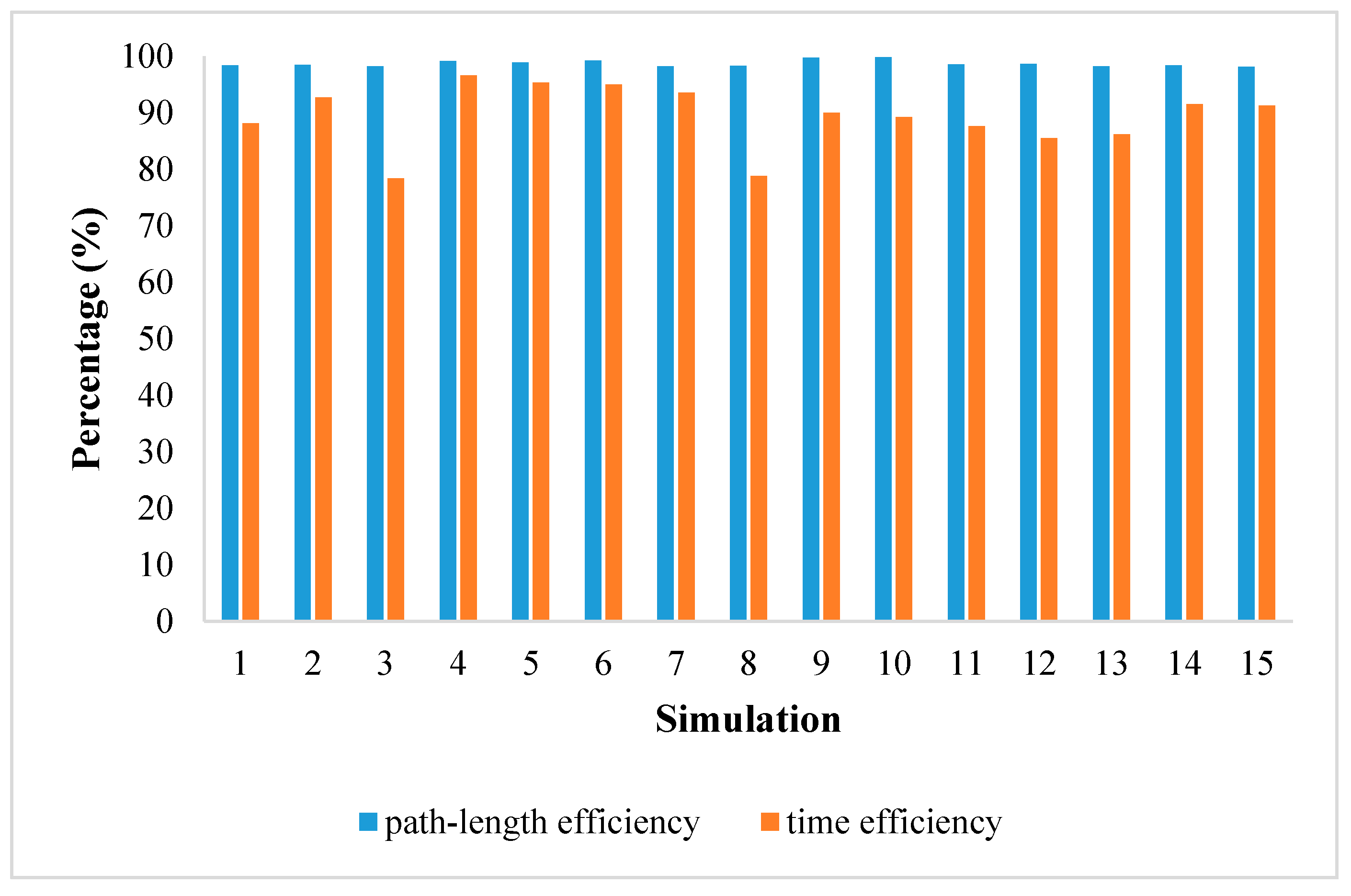
| Path-length efficiency (%) | 99.81 | 98.15 | 0.31 | 98.67 |
| Time-efficiency (%) | 96.61 | 78.42 | 29.97 | 89.32 |
Publisher’s Note: MDPI stays neutral with regard to jurisdictional claims in published maps and institutional affiliations. |
© 2021 by the authors. Licensee MDPI, Basel, Switzerland. This article is an open access article distributed under the terms and conditions of the Creative Commons Attribution (CC BY) license (http://creativecommons.org/licenses/by/4.0/).
Share and Cite
Zong, F.; Zeng, M.; Cao, Y.; Liu, Y. Local Dynamic Path Planning for an Ambulance Based on Driving Risk and Attraction Field. Sustainability 2021, 13, 3194. https://doi.org/10.3390/su13063194
Zong F, Zeng M, Cao Y, Liu Y. Local Dynamic Path Planning for an Ambulance Based on Driving Risk and Attraction Field. Sustainability. 2021; 13(6):3194. https://doi.org/10.3390/su13063194
Chicago/Turabian StyleZong, Fang, Meng Zeng, Yang Cao, and Yixuan Liu. 2021. "Local Dynamic Path Planning for an Ambulance Based on Driving Risk and Attraction Field" Sustainability 13, no. 6: 3194. https://doi.org/10.3390/su13063194
APA StyleZong, F., Zeng, M., Cao, Y., & Liu, Y. (2021). Local Dynamic Path Planning for an Ambulance Based on Driving Risk and Attraction Field. Sustainability, 13(6), 3194. https://doi.org/10.3390/su13063194