Abstract
Troop movement involves transporting military personnel from one location to another using available means. To minimize damage from enemies, the military simultaneously uses reconnaissance and transportation units during troop movements. This paper proposes a vehicle routing problem considering reconnaissance and transportation (VRPCRT) for wartime troop movements. The VRPCRT is formulated as a mixed-integer programming model for minimizing the completion time of wartime troop movements and reconnaissance, and transportation vehicle routes were determined simultaneously in the VRPCRT. For this paper, an ant colony optimization (ACO) algorithm for the VRPCRT was also developed, and computational experiments were conducted to compare the ACO algorithm’s performance and that of the mixed-integer programming model. The performance of the ACO algorithm was shown to yield excellent results even for the real-size problem. Furthermore, a sensitivity analysis of the change in the number of reconnaissance and transportation vehicles was performed, and the effects of each type of vehicle on troop movement were analyzed.
1. Introduction
Troop movement involves transportation of military personnel from one location to another using available means. In wartime, rapid and efficient troop movement offers many benefits in battle. For instance, efficient troop movement saves time and resources, which can be used for combat preparation and future operations. To win a battle, the commander must concentrate combat power at the opportune place and time to achieve a relative advantage over the enemy. Therefore, in the process of rearranging troops, efficient and rapid movement is essential.
Because the situations are uncertain during wartime, the commander makes a lot of efforts to reduce the uncertainty, and reconnaissance is one of the efforts to reduce the uncertainty. During troop movement, a surprise attack by an unexpected enemy at a specified area is a major threat (uncertainty) for the commander. To avoid this uncertainty, the commander deploys his reconnaissance units before troop movement to conduct patrol specified area, and gathers information to reduce uncertainty through reconnaissance units. The prevention of surprise and the gathered information through reconnaissance makes the wartime situation relatively stable and static for the commander. In other words, reconnaissance is an essential process to turn an uncertain situation into a stable and static situation, which is also stated in the field manual. Therefore, when performing reconnaissance before troop movement, a static and stable wartime situation can be assumed.
The procedure for tactical troop movement in wartime consists of two parts. First, the reconnaissance troops patrol the area where the units and equipment will be transported. Second, the transportation troops move the units and equipment to the area where the reconnaissance troops have patrolled. Because of enemy threats, such as an ambush or surprise attack, the reconnaissance troops are deployed to protect the vehicle movement undertaken by the transportation unit during an operation. Figure 1 represents an example of the procedure for tactical troop movement in wartime.
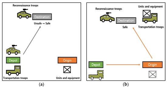
Figure 1.
(a) Reconnaissance troops patrol the destination; (b) Transportation troops move units and equipment at the destination.
Troop movement is usually performed using a ground vehicle or helicopter, and in some cases, the troops move on foot. Troop movement using vehicles is associated with the vehicle routing problem (VRP) and the pickup and delivery problem (PDP). The VRP and the PDP have been studied for approximately 30 years and have been used in many areas of study. Swersey and Ballard [1] introduced a school bus-routing problem. Yan and Chen [2] applied the PDP to a carpooling system. Koc and Karaoglan [3] studied green vehicle routing problems, which emphasize environmental protection in logistical activity. Zhang and Xiong [4] dealt with a grain emergency vehicle scheduling problem for grain distribution in a disaster area and developed a hybrid algorithm combining artificial immune and ant colony optimization algorithm. Vincent et al. [5] proposed a hybrid vehicle routing problem (HVRP), in which plug-in hybrid electric vehicles were considered. They developed simulated annealing heuristic algorithm for the HVRP. Koç et al. [6] studied an electric vehicle routing problem. In their problem, shared charging stations were considered. Calvet et al. [7] studied a stochastic multi depot vehicle routing problem in which limited fleets of vehicles are available to reflect practical situations.
Chemla et al. [8] studied an M-M type of PDP for bike-sharing systems. In their study, only one commodity and a capacitated single vehicle were allowed to visit a node several times. The authors proposed an efficient algorithm for the problem and a theoretical result concerning the algorithm. Dumas et al. [9] studied a pickup and delivery problem with time windows (PDPTW), which is a generalized VRP. In the problem, a vehicle route satisfies constraints, such as those related to transportation requests, capacity, time windows, and precedence. They presented an exact algorithm using column generation. Lau and Liang [10] proposed a two-phase-method algorithm for the PDPTW. In the first phase, the algorithm was constructed by combining an insertion and a sweeping heuristic to obtain an initial solution. In the second phase, a tabu search was used for improving the initial solution.
Cordeau [11] dealt with a dial a ride problem (DARP). In the problem, various constraints, such as capacity, duration, paring, precedence, and time window constraints, were considered and introduced in a mixed-integer programming (MIP) formulation. A branch-and-cut algorithm, based on new valid inequalities for the DARP, was introduced. Malapert et al. [12] studied the PDP with two-dimensional loading constraints in which items were two-dimensional rectangles. Männel and Bortfeldt [13] proposed a PDP with three-dimensional loading constraints (3L-PDP). In the 3L-PDP, the vehicle capacity and requests were expressed in the form of a three-dimensional rectangle. They used a hybrid algorithm for the model. Pankratz [14] came up with a grouping-genetic algorithm for the PDPTW.
Montané and Galvao [15] dealt with the VRP using simultaneous pickup and delivery (VRPSPD) and developed a tabu search algorithm for it. Chen and Wu [16] also studied the VRPSDP and suggested a new hybrid heuristic algorithm by combining record-to-record travel and tabu lists. Çatay [17] introduced an effective ACO algorithm for the VRPSPD.
After the PDP was introduced, heuristic and meta-heuristic algorithms for solving it were developed. Lu and Dessouky [18] presented a new insertion-based construction heuristic for the PDPTW. The crossing-length percentage (CLP), which is used to quantify the visual attractiveness of the solution, was introduced in their study. The CLP used in their heuristic algorithm improved the quality of the solution. Computational experiments showed that the proposed heuristic was better than a sequential-insertion heuristic and a parallel-insertion heuristic. Melachrinoudis et al. [19] proposed a double-request DARP with soft time windows and suggested a tabu search heuristic as the solution method.
Ruiz et al. [20] developed a biased random-key genetic algorithm for the open vehicle routing problem with capacity and distance constraints. They tested their algorithm through three sets of benchmark problems. Salavati-Khoshghalb et al. [21] studied the vehicle routing problem with stochastic demands under an optimal restocking policy. They developed an exact algorithm which modified the integer L-shaped algorithm to solve the problem. Pasha et al. [22] proposed an optimization model for the vehicle routing problem with a “factory-in-a-box”. They developed an evolutionary algorithm to solve the problem and performed numerical experiments to test their algorithm’s performance by comparing three meta-heuristic algorithms, including tabu search, variable neighborhood search, and simulated annealing.
Zhang et al. [23] dealt with a multi-objective vehicle routing problem with flexible time windows. They developed a solution method combining an ant colony optimization and three mutation operators. Trachanatzi et al. [24] introduced the environmental prize-collecting vehicle routing problem (E-PCVRP), which was extended from the prize collecting vehicle routing problem. In the E-PCVRP, the objective is CO2 emissions minimization, not cost minimization of the total distance traveled. They developed the firefly algorithm based on coordinates to solve the E-PCVRP. Theeb et al. [25] optimize a logistic plan considering the electric vehicle routing problem, and Huang et al. [26] studied the routing problem in global production planning.
Metaheuristics and nature-inspired algorithms have been widely used to solve complex decision problems in various domains such as scheduling, medicine, data classification, multi-objective optimization, and online learning. Their performance has been proved through numerous studies
Dulebenets [27] studied a truck scheduling problem at a cross-docking facility and developed a delayed start parallel evolutionary algorithm to solve the problem. D’Angelo et al. [28] used genetic programming to distinguish bacterial and viral meningitis. Panda and Majhi [29] proposed a salp swarm algorithm(SSA) that trained the multilayer perceptron for the task of data classification. Liu et al. [30] proposed a many-objective evolutionary algorithm consisting of an angle-based selection strategy and a shift-based density estimation strategy to solve many objective optimization problems. Zhao and Zhang [31] studied online learning based evolutionary many-objective algorithm. Shimizu and Sakaguchi [32] developed hybrid meta heuristic algorithm considering multi depot VRP.
Ant colony optimization (ACO) algorithm is developed among various meta-heuristic algorithms to solve the traveling salesman problem (TSP) and the VRP efficiently. As the ACO algorithm was first proposed, many ACO variations have been developed to solve the VRP faster and more efficiently. Dorigo et al. [33] introduced the ant system (AS), the first ACO algorithm used to solve the TSP. They compared it with other meta-heuristics, such as the tabu search, simulated annealing, and a genetic algorithm. Hu et al. [34] developed the continuous orthogonal ant colony, in which the orthogonal design method was used to search the solutions effectively.
Dorigo and Gambardella [35] introduced the ACS, which was extended from the AS. The local pheromone updating rule and new state transition rule were applied to the ACS. Stützle and Hoos [36] developed the MAX–MIN ant system (MMAS), which was derived from the AS. Only the best ants, found globally, were used to update the pheromone trails, which were limited for each solution to avoid stagnation in the MMAS. Blum and Dorigo [37] introduced the hyper-cube of the ACO, in which the pheromone value was limited between 0 and 1. Favaretto et al. [38] developed the ACS for the VRP with multiple time windows. Fuellerer et al. [39] studied the two-dimensional loading-vehicle routing problem and the proposed ACO algorithm based on the AS. Yousefli [40] developed the fuzzy AC approach to consider the project scheduling problem. Tchoupo et al. [41] developed a meta-heuristic based on the ACO combined with dedicated local search algorithms for the PDPTW.
In this study, transportation and reconnaissance troops (vehicles) are considered simultaneously, and their routes are needed to be coordinated. Bae and Moon [42] extended a multi-depot VRP by considering two different types of service vehicles: delivery and installation. The service level, which refers to the time interval between delivery and installation, was proposed in the model. They also developed a new hybrid genetic algorithm. Aldaihani and Dessouky [43] studied the problem, which deals with integrating fixed route service (buses) and general PDP (taxis). They proposed a three-stage heuristic construction algorithm that provides an approximate solution. The differences among VRP studies that deal with multi types of vehicles performing different tasks are summarized in Table 1.

Table 1.
Characteristics of literature review.
The VRPCRT is NP-hard, because it is a generalization of PDP. Due to complexity of NP-hard, many heuristic algorithms were developed to solve it. An ant colony optimization (ACO) algorithm based on the ant colony system (ACS) was proposed to solve the VRPCRT in this study.
The contribution of this paper is as follows. First, we applied the VRP to the military field. Koo and Moon [44] introduced a wartime logistic model considering frontline change to contribute the military field. However, their model was developed using a location allocation problem, not the vehicle routing problem. VRPs are frequently used in real-life peacetime situations, such as those related to transportation or logistic systems. Despite clear applications for wartime, fewer VRPs have been used to study military situations compared to the implementation and research of them for peacetime, such as with transportation or logistic systems. For the study described in this paper, by applying the VRP to the military field, procedures of troop movement were modeled with the VRPCRT.
Second, the VRPCRT was extended from the traditional PDP. During troop movement in wartime, reconnaissance troops (vehicles) have to visit destinations only for patrol, and transportation troops (vehicles) have to visit origins to carry units before moving to destinations. In other words, the reconnaissance and transportation vehicles move in the form of traditional VRP and PDP, respectively. In the traditional VRP and PDP, a single type of vehicle routes was determined. However, transportation and reconnaissance vehicle routes were determined simultaneously in the VRPCRT. Constraints, such as pairing or precedence, in the PDP were included in the VRPCRT. Of note, in the VRPCRT, transportation vehicle routes were influenced by reconnaissance vehicle routes according to the procedure of troop movement; this condition was formulated as a time window constraint.
Third, this study could contribute to wartime logistics’ sustainability by providing efficient vehicle routes for troop movements. Several studies that were related to sustainability focused on the efficient use of resources and environmental impacts. Especially, electric and green vehicle problems, which are intended to have less environmental impact, are studied. VRPs related to carpooling or carsharing could also contribute to sustainability from the point of resource saving.
In this study, reconnaissance and transportation vehicle routes for efficient troop movements in wartime were determined, and efficient troop movements could be expected to save many resources in wartime. In other words, even though the VRPCRT did not consider environmental factors directly as electric or green vehicles, the VRPCRT could be regarded as a contribution to sustainability.
2. Problem Formulation
2.1. Problem Description and Assumptions
This study was aimed at developing a model for tactical troop movement in wartime. The model was developed on a complete network. The node set, W, is partitioned into {J, P, D}, for which J = {0} is the depot, P = {1, 2, …, n} is the set of origin nodes, and D = {n + 1, …, 2n} is the set of destination nodes. Each arc is associated with travel time, . For the PDP, a request specifies the locations where people are picked up and where they are delivered [34]. The request described for the PDP applies equally to the VRPCRT. Each node i ∈ W is associated with the loading requirement (in some military units), , and the boarding and disembarking time, , such that . Each node i ∈ D is associated with the reconnaissance time, . Set K contains reconnaissance vehicles with a maximum route time, , and set S consists of transportation vehicles. Each transportation vehicle has capacity, , and maximum route time, . Dual time windows were used for destination nodes.
A time window [0, ] for the reconnaissance vehicle is associated with node i∈ D, for which refers to the latest time for reconnaissance. A time window [ + ,] for the transportation vehicle is associated with node i ∈ D for which and represent the latest time for transportation and arrival time of the reconnaissance vehicle, respectively. The time windows for transportation indicate that transportation vehicles can visit only destination nodes that have been patrolled by a reconnaissance vehicle.
The transportation vehicle in the troop movement procedure is similar to that of the PDP, which was designed to determine a route and schedule for pickup and delivery requests between origin and destination pairs [11]. In the PDP, the route of the transportation vehicle satisfies the precedence, pairing, capacity, maximum route time, and time window constraints. The precedence constraint means that a vehicle visits the origin before moving to a destination, and a pairing constraint is used so that the customer’s pickup and delivery request is fulfilled by the same vehicle [45]. Figure 2 shows an example of requests and a vehicle route that satisfies the precedence and pairing constraints.
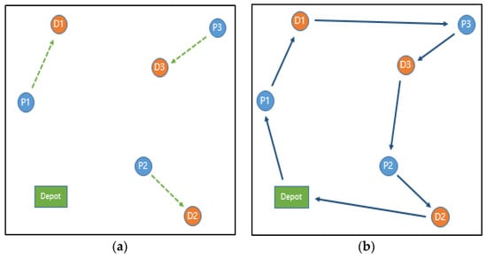
Figure 2.
(a) Origin and destination of each request; (b) Vehicle route satisfying paring and precedence constraints.
In the VRPCRT, reconnaissance vehicles visited only the destination nodes and necessarily satisfied the time window and maximum route time constraints. This reconnaissance activity at a destination during troop movement was performed by reconnaissance troops. Transportation vehicles satisfied the constraints of the PDP, such as pairing, precedence, capacity, and time window constraints, and thus were used in the VRPCRT to describe the transportation troops that move units and equipment from an origin to a destination.
Figure 3 represents the feasible routes for the reconnaissance and transportation vehicle in the VRPCRT. Figure 3 shows that the transportation vehicle waits at the P1 node until the reconnaissance vehicle leaves the D1 node, and then it visits the D1 node after the reconnaissance vehicle at the D1 node has advanced to the D3 node. If the reconnaissance vehicle at the D1 node is delayed, then the arrival time for transportation vehicle at the D1 node is also delayed. Hence, the transportation vehicle route was affected by the reconnaissance vehicle route because of the time window constraints of transportation, as explained in the previous paragraph. In other words, the time windows of the transportation vehicles in the VRPCRT were not given as parameters, because they depended on the reconnaissance vehicle routes.
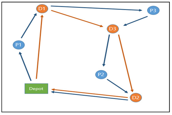
Figure 3.
The VRPCRT model.
The following assumptions about the model were used to develop the VRPCRT:
- (1)
- Two types of vehicles (reconnaissance and transportation) and two types of nodes (origin and destination) were used.
- (2)
- A single depot was used, and all vehicles departed from and returned to the depot.
- (3)
- Destination nodes must be visited exactly once by a reconnaissance vehicle, and origin and destination nodes must be visited once by a transportation vehicle.
- (4)
- A transportation vehicle can only visit a destination node that has been patrolled by a reconnaissance vehicle.
- (5)
- Requests of each troop must be served by a transportation vehicle.
- (6)
- Loading requirement (in some military units) at all nodes cannot exceed the capacity of the transportation vehicle.
- (7)
- All vehicles must satisfy the time window constraints of each node and the maximum route time constraints.
2.2. Model Formulation
An MIP model was developed for troop movement in wartime. Sets, parameters, and decision variables of the model are described as follows:
Sets
P: set of origin nodes for requests, P = {1, 2, 3, …, n} where n is the total number of requests
D: set of destination nodes for requests, D = {n + 1, n + 2, …, 2n} where n is the total number of requests
J: depot, J = {0}
W: set of all nodes, W = P ∪ D ∪ J
K: set of reconnaissance vehicles
S: set of transportation vehicles
U: P ∪ D
Decision variables
: arrival time of the reconnaissance vehicle at node i ∀ i ∈ D
: arrival time of the transportation vehicle at node i ∀ i ∈ U
: arrival time of the reconnaissance vehicle at the depot ∀ j ∈ J, k ∈ K
: arrival time of the transportation vehicle at the depot ∀ j ∈ J, s ∈ S
∀ i, j ∈ D∪J, k ∈ K
∀ i, j ∈ W, s ∈ S
: loading requirement (in some military units) in transportation vehicle S after visiting node i ∀ i ∈ U, s ∈ S
Parameters
: latest time for reconnaissance at node i ∀ i ∈ D
: latest time for transportation at node i ∀ i ∈ D
: travel time between nodes i and j ∀ i, j ∈ W
: loading requirement to board at node i ∀ i ∈ P
: loading requirement that disembark at node i () ∀ i ∈ D
: reconnaissance time at node i ∀ i ∈ D
: boarding and disembarking times at node i ∀ i ∈ U
: maximum route time for vehicle k ∀ k ∈ K
: maximum route time for vehicle s ∀ s ∈ S
: capacity for vehicle s ∀ s ∈ S
M: big M
The formulation of the VRPCRT can be stated as follows:
Minimize τ
| (1) | ||
| (2) | ||
| (3) | ||
| . | (4) | |
| (5) | ||
| (6) | ||
| (7) | ||
| (8) | ||
| (9) | ||
| (10) | ||
| (11) | ||
| (12) | ||
| (13) | ||
| (14) | ||
| (15) | ||
| (16) |
The objective function minimizes the maximum arrival time of any transportation vehicle. Because it is important to minimize the total distance from a cost perspective in peacetime, in most of VRPs, the objective function is to minimize the total distance traveled by vehicles. However, the VRPCRT is a model for troop movement in wartime, and it is most important to complete the mission quickly in wartime. The completion time of troop movement is the time at which all units arrive at their designated destination, and objective function should be selected as shown in the formulation of the VRPCRT to terminate troop movement as soon as possible. If the objective function of the VRPCRT is to minimize the total distance traveled by vehicles, the completion time of troop movement may be longer. This could be fatal in wartime. Constraint (2) represents the destination nodes that must be visited exactly once by a reconnaissance vehicle. Constraint (3) indicates that the origin and destination nodes must be visited once by a transportation vehicle. Constraints (4) and (5) ensure that the vehicle that visited the node is the same vehicle that is leaving the node. Constraints (6) and (7) refer to the reconnaissance and transportation vehicle, respectively, that depart from the depot. Constraint (8) indicates that each request is served by the same transportation vehicle. Constraint (9) guarantees that the transportation vehicle visits the origin nodes before the destination nodes. Constraints (10) and (11) represent relationships between the arrival time of the reconnaissance and transportation vehicles to nodes. Constraints (12) and (13) are related to the maximum route time for the reconnaissance and transportation vehicles. Constraints (14) and (15) specify the time window constraints, and constraint (16) dictates the vehicle capacity constraint.
2.3. Numerical Example
In this section, the VRPCRT was validated by solving the numerical example through Xpress-IVE Version 1.24 (http://www.fico.com, accessed on 24 August 2018) optimization software. Small data sets consisting of seven nodes are presented in the numerical example. The nodes in this example consist of three origins, three destinations, and one depot. Travel times between each node and the parameters for the model are presented in Table 2 and Table 3, respectively. All parameters for this example were generated randomly.
Table 2.
Travel times between nodes in the numerical example.
Table 3.
Parameters in the numerical example.
The routes and arrival times of each vehicle are described in Table 4 and illustrated in Figure 4. The optimal value provided by the model was 228, which refers to the completion time of the troop movement. Transportation vehicles satisfied the precedence, paring, and capacity constraints in the numerical example, and both transportation and reconnaissance vehicles satisfied the time window and the maximum route time constraints in the numerical example.
Table 4.
Results from the numerical example.
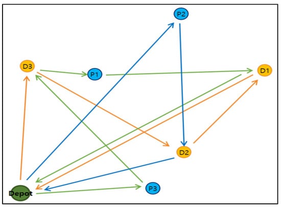
Figure 4.
Each vehicle routes in the numerical example.
The main feature of the VRPCRT is that the reconnaissance vehicle route affects the route of the transportation vehicle. In other words, transportation vehicles must visit the destination nodes that the reconnaissance vehicles have patrolled. In this example, all transportation vehicles visited the destination nodes after the reconnaissance vehicles completed the assignment such that transportation vehicle 1 waited at the P1 node until after the reconnaissance vehicle completed duty at the D1 node.
3. Ant Colony Optimization Algorithm
In this section, the proposed ACO algorithm for the VRPCRT is described. The ACO algorithm is a meta-heuristic developed to solve combinatorial optimization problems, such as the TSP or VRP. The ACO algorithm was based on the idea that ants leave pheromone trails when they are searching for food. The pheromone affects the way the ants move, so it is an important factor for the ACO algorithm. In the natural world, the pheromone accumulates along the route of ants searching for food or evaporates over time. Similarly, the pheromone accumulates or evaporates according to the parameters and rules of the ACO algorithm.
The proposed ACO algorithm for the VRPCRT in the study is based on the ACS algorithm that features the local pheromone updating and transition rule that differs from the AS [46]. The proposed ACO algorithm was also modified by considering characteristics of the VRPCRT.
The process for running the ACO algorithm for the VRPCRT consists of three steps. The first step involves construction of a solution such that the ants (vehicles) select each node probabilistically and repeats this process until feasible solutions (routes) were generated. The second step requires local pheromone updating. Whenever ants constructed a feasible solution, local pheromone updating was performed to change the probability that the ants would choose each node. In the third step, the global pheromone updating is performed. It affected the probability that ants would select each node according to the best solution, which had been constructed in the first step. The three steps of the proposed ACO algorithm were repeated as described to discover and improve feasible solutions. The procedure for the developed ACO algorithm is as shown in Algorithm 1.
3.1. Construction of a Solution
In this section, the process of construction of a solution is described. For the PDP, only the routes of the transportation vehicles are considered as the feasible solutions. Meanwhile, the model presented in this paper takes into account both reconnaissance and transportation vehicles simultaneously, so the feasible solution refers to route pairs of reconnaissance and transportation vehicles that satisfy the constraints.
For the creation of a feasible solution for the VRPCRT, a reconnaissance vehicle route was made. Then, the transportation vehicle route was determined according to the reconnaissance vehicle route. Because the time window constraints of the transportation vehicle were affected by the reconnaissance vehicle route, the reconnaissance vehicle route must be fixed first to determine the transportation vehicle route.
In the ACO algorithm, vehicles are represented by ants. Therefore, for this study, reconnaissance and transportation ants represent reconnaissance and transportation vehicles, respectively. The reconnaissance route was made as follows: the number of ants (vehicles) was given, and every reconnaissance ant was located at the depot. One of the ants is selected randomly. It selects one of the feasible nodes that can visit from its current node through transition rule and adds the feasible node to its route. The next ant, also selected randomly, moves to a feasible node and creates a route, different from the first ant, by adding feasible nodes. This process was repeated until the reconnaissance ants (vehicles) visit all the destination nodes and satisfy all the constraints at the same time. The reconnaissance routes were thus created by the time the process was ended. After the reconnaissance routes were made, transportation routes were made in the same way.
Whenever it adds a feasible node to its route, the ant (vehicle) follows the transition rule for constructing a route [47]: The ant selects the node with the highest value with probability . If the node with the highest value is not selected (with probability 1 − ), then the ant selects another node j with probability as follows:
In this equation, represents the set of feasible nodes when ant k is positioned at node i. The term stands for a pheromone between node i and j. The ηij value is a heuristic reciprocal of the time value for travel between node i and j. The parameters are q0, α, and β. In addition, several feasible solutions were generated by repeating the first step in each iteration of the ACO algorithm.
3.2. Pheromone Updating
The pheromone affects how ants move in the natural world. Therefore, for the ACO algorithm, the pheromone affects the node selection of ants (vehicles). Because the probability of node selection in construction of a solution depends on the pheromone, the probability of node selection changes as the pheromone updating progresses. For the VRPCRT, and refer to the respective pheromones between node i and j for the reconnaissance and transportation ants. The pheromones are distinguished in the ACO algorithm to create various feasible solutions in the first step. Pheromones for reconnaissance and transportation ants are updated, independently. Two types of pheromone updating were used for the ACO algorithm: local and global.
Local pheromone updating was performed whenever a feasible solution was generated in the first step. When the reconnaissance and transportation ants visit node j from node i along the feasible solution (route), local pheromone updating was performed as follows [47]:
The initial pheromones for the reconnaissance and transportation ant (vehicle) are and , respectively, and is a parameter to control the evaporation rate during local pheromone updating. The first step and local pheromone updating were repeated several times for each iteration. When first step and local pheromone updating finished in an iteration, the global pheromone updating was performed. When global pheromone updating is processed, only the best solution is required. The best solution is the feasible solution that has the minimum objective value among the feasible solutions generated from the iteration.
Therefore, global pheromone updating was executed only once for each iteration. When the reconnaissance and transportation ant (vehicle) visits node j from node i using the best solution (the best route), global pheromone updating was performed as follows [36]:
The term Q refers to a parameter, and is the objective function value for the best route in the kth iteration.
| Algorithm 1. Procedure of ACO Algorithm for the VRPCRT |
| Input parameters for ACO algorithm(, , , , , ) , : initial pheromones I: number of iterations that algorithm repeated A: number of feasible solutions in each iteration Output final_sol, final_value |
| 1: begin algorithms |
| 2: initialize final_sol, final_value, , |
| 3: for = 1 to I |
| 4: initialize , best_sol, best_value |
| 5: for = 1 to A // Construction of a solution |
| 6: while do // Construction of reconnaissance vehicle route |
| 7: Select one of reconnaissance ant k |
| 8: Move ant k to a feasible node with transition rule |
| 9: until = { } for all k |
| 10: while do // Construction of transportation vehicle route |
| 11: Select one of transportation ant s |
| 12: Move ant s to a feasible node with transition rule |
| 13: until = { } for all s |
| 14: Get feasible value and feasible solution // |
| 15: Local pheromone update // updating based on feasible solution |
| 16: If feasible value then |
| 17: feasible value |
| 18: best_sol ⟵ feasible solution |
| 19: end for |
| 20: best_value ⟵ . |
| 21: Global pheromone update // updating based on best_sol |
| 22: If final_value best_value |
| 23: final_value ⟵ best_value |
| 24: final_sol ⟵ best_sol: |
| 25: end for |
| 26: End algorithm |
4. Computational Experiment
In this section, the computational experiment for the model is presented. The discussion consists of two parts. First, a comparison is described for the performance between the proposed ACO algorithm and a MIP model. The MIP model was solved with Xpress-IVE Version 1.24, and the ACO algorithm was coded by JAVA Eclipse. Second, a sensitivity analysis on the changes in the number of vehicles is explained. All computational experiments were conducted by a computer featuring 8GB RAM and Intel(R) Core (TM) i5-3470 CPU with 3.20 GHz.
4.1. Parameter Tuning
Because the performance of metaheuristic algorithm is greatly affected by the parameter values, it is important to estimate appropriate parameter values. Before executing the proposed ACO algorithm, parameter tuning analysis was conducted to estimate the appropriate parameter values. The best process for tuning analysis is to confirm the performance of ACO algorithm for combination of every parameter values. However, this process for tuning analysis is difficult to conduct due to many combinations. Tuning analysis was performed to estimate the appropriate parameter value. First, we generated the test sample for tuning analysis and found the optimal solution for the test sample. Second, for the test sample, the eight parameters were adjusted randomly until the ACO algorithm found the optimal solution. Third, the parameters used when the optimal solution was found were selected as appropriate parameters. The selected parameters of the ACO algorithm are presented in Table 5.
Table 5.
Parameters for Experiment 1.
4.2. Experiment 1
For the first part of the experiment, the performance of the proposed ACO algorithm was verified. Data sets for the computational experiment were randomly generated. Parameters of the ACO in Table 5 are used, and the results of the computational experiment are shown in Table 6, Table 7 and Table 8. Each experiment consisted of 10 instances. The ACO algorithm was run 10 times for each instance.
Table 6.
Experiment 1 results with 13 nodes.
Table 7.
Experiment 1 results with 15 nodes.
Table 8.
Experiment 1 results with 17 nodes.
As shown in Table 6, the optimal value of each instance was found by the MIP Model through Xpress-IVE. The optimal solution was acquired within 30 s, and the ACO algorithm solution was found immediately. The gap between the optimal value and the value found by the ACO was within 1%.
For the case of 15 nodes, the computational experiment time was limited to 7200 s per instance, and the optimal solution was obtained for seven of 10 instances. The optimal value and experiment time for the MIP, conducted through Xpress-IVE, are presented in Table 7. The ACO algorithm found a feasible solution within 20 s for all instances, and the gap was within 5% for the instance in which the optimal solution was obtained. The ACO algorithm found better solutions than the feasible solutions obtained by the MIP model using Xpress-IVE within 7200 s for the instances that did not reach an optimal solution (instance 15-2, 8)
The computational experiment time also was limited to 7200 s for the case of 17 nodes. The results are presented in Table 8. The optimal solution was obtained for only one of 10 instances (instance 17-3), and feasible solutions were found for the other instances. The ACO algorithm found the solution within 60 s and found the optimal solution in instance 17-3. In some instances (17-1, 2, 4, 6, 7, 9, and 10), the ACO algorithm found better feasible solutions than the MIP model that was conducted using Xpress-IVE.
4.3. Experiment 2
The second experiment was a sensitivity analysis related to the changing number of vehicles. The change in the number of vehicles can be divided into three cases: (1) the number of reconnaissance vehicles remained constant and the number of transportation vehicles changed, (2) the number of transportation vehicles remained constant and the number of reconnaissance vehicles changed, and (3) the total number of vehicles remained constant and the ratio of reconnaissance to transportation vehicles changed. The ACO algorithm was used for sensitivity analysis. Data sets and parameters for this experiment were randomly generated. Cases 1 and 2 each featured 21 nodes, and the Case 3 featured 51 nodes. The computational experiments for the sensitivity analysis were limited to 300 s.
The parameters of Experiment 2 for the ACO are presented in Table 9. The parameters used in Experiment 2 are different from those in Experiment 1. Experiment 1 was computational experiment to confirm the performance of the proposed ACO algorithm. However, Experiment 2 was a computational experiment to confirm the change in trend of the objective function according to the number of vehicles. Therefore, parameters “A” and “I” were adjusted so that the experiment could be terminated quickly within a limited time.
Table 9.
Parameters for Experiment 2.
Table 10 shows the results of the sensitivity analysis for Case 1, and Figure 5 presents graphs showing the average results of Case 1: as the number of transportation vehicles increased, the completion time for troop movements also decreased. Additionally, the rate of change of the completion time for the troop movement decreased as the number of transportation vehicles increased.
Table 10.
Sensitivity analysis results for Case 1.
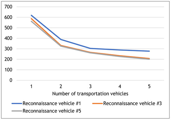
Figure 5.
Sensitivity analysis results for Case 1.
Table 11 shows the sensitivity analysis results for Case 2, and Figure 6 features graphs showing the average results of Case 2: As the number of reconnaissance vehicles increased, the completion time for troop movement also decreased. However, the rate of change of completion time for the troop movement did not change significantly when the number of reconnaissance vehicles was increased.
Table 11.
Sensitivity analysis results for Case 2.
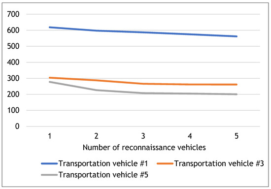
Figure 6.
Sensitivity analysis results for Case 2.
Table 12 and Figure 7 present the sensitivity analysis results for Case 3. As shown in Figure 7, the experimental results of Case 3 generally took a convex shape. The proportion of the transportation vehicle was confirmed as necessarily greater than the reconnaissance vehicle proportion to minimize the completion time for troop movement when the total number of vehicles remained constant. The completion time for troop movement increased as the number of transportation vehicles decreased when the proportion of the reconnaissance vehicles was greater than the proportion of transportation vehicles. According to the sensitivity analysis results, the completion time for troop movement decreased as the total number of vehicles increased, and the number of transportation vehicles was found to have exerted greater influence on the completion time of troop movement than did the number of reconnaissance vehicles.
Table 12.
Sensitivity analysis results for Case 3.
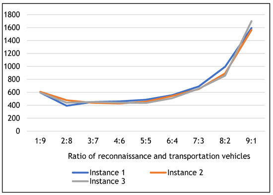
Figure 7.
Sensitivity analysis results for Case 3.
5. Conclusions
In a major contribution from this study, the new model for troop movement in wartime was developed by extending the PDP. The following differences characterize the PDP and the VRPCRT: In the PDP, only transportation vehicles are considered, and the transportation vehicle routes are determined using various constraints. Time windows for transportation vehicles at each node are deterministic as parameters in the PDP. In the VRPCRT, as proposed in this study, reconnaissance and transportation vehicles were considered, and both vehicle routes were determined simultaneously.
This study could be considered a sustainability contribution for wartime logistics by providing efficient vehicle routes for troop movements. The VRPCRT was developed to save and efficiently use resources for troop movements in wartime, and through the VRPCRT, efficient troop movements and resource saving could be possible.
In this study, the VRPCRT, which is the mathematical model for determining tactical troop movements, and the ACO algorithm were developed. The ACO algorithm’s performance was tested through computational experiments and was shown to yield excellent results, even for the real-sized problem. The sensitivity analysis on the number of vehicles was performed using the ACO algorithm developed for the model. The troop movement in wartime was sensitive to the number of transportation vehicles.
A sensitivity analysis related to the number of vehicles was performed, and it confirmed that the transportation vehicles affected troop movement more than the reconnaissance vehicles did. If the size of the input data for computational experiments is increased or the maximum running time for solving the problem is extended, it could be thought that a better insight may be derived.
The limitation of this paper is as follows. First, the performance of the ACO algorithm is influenced greatly by the chosen parameters. However, optimal parameters of the proposed ACO algorithm were not suggested in this paper. Second, drones, unmanned aerial vehicles (UAVs), satellites, helicopters, and many other types of equipment are used for reconnaissance in wartime situations. However, only reconnaissance vehicles were considered in the VRPCRT. Future studies may include the following:
- Studies on metaheuristics, selecting optimal parameters for the proposed ACO algorithm proposed in this paper, are also suggested.
- Military UAV and the associated features (e.g., wide observation range) could be studied for the VRPCRT.
- Multiple depots for reconnaissance and transportation vehicles could be considered in the VRPCRT.
- An alternative metaheuristic algorithm for the VRPCRT could be developed (e.g., genetic algorithm, tabu search algorithm, simulated annealing algorithm).
Author Contributions
Conceptualization, I.M. and B.J.; methodology, I.M., M.KIM and B.J.; software, B.J.; validation, M.K.; formal analysis, I.M. and M.K.; investigation, M.KIM and B.J.; resources, M.KIM and B.J.; data curation, B.J.; writing—original draft preparation, B.J.; writing—review and editing, I.M. and M.K.; visualization, B.J.; supervision, I.M. and M.K.; project administration, I.M.; funding acquisition, I.M. All authors have read and agreed to the published version of the manuscript.
Funding
This research was supported by National Research Foundation of Korea (NRF), funded by the Ministry of Science, ICT, and Future Planning [grant number NRF-2019R1A2C2084616].
Institutional Review Board Statement
Not applicable.
Informed Consent Statement
Not applicable.
Data Availability Statement
Please contact corresponding author. The data used in this paper are hypothetical data, independent of the actual military or private enterprise data.
Acknowledgments
The authors would like to thank three anonymous reviewers for their thoughtful comments and suggestions on the manuscript.
Conflicts of Interest
The authors declare no conflict of interest.
References
- Swersey, A.J.; Ballard, W. Scheduling school buses. Manage. Sci. 1984, 30, 844–853. [Google Scholar] [CrossRef]
- Yan, S.; Chen, C.-Y. An optimization model and a solution algorithm for the many-to-many car pooling problem. Ann. Oper. Res. 2011, 191, 37–71. [Google Scholar] [CrossRef]
- Koç, Ç.; Karaoglan, I. The green vehicle routing problem: A heuristic based exact solution approach. Appl. Soft Comput. 2016, 39, 154–164. [Google Scholar] [CrossRef]
- Zhang, Q.; Xiong, S. Routing optimization of emergency grain distribution vehicles using the immune ant colony optimization algorithm. Appl. Soft Comput. J. 2018, 71, 917–925. [Google Scholar] [CrossRef]
- Vincent, F.Y.; Redi, A.A.N.P.; Hidayat, Y.A.; Wibowo, O.J. A simulated annealing heuristic for the hybrid vehicle routing problem. Appl. Soft Comput. 2017, 53, 119–132. [Google Scholar]
- Koç, Ç.; Jabali, O.; Mendoza, J.E.; Laporte, G. The electric vehicle routing problem with shared charging stations. Int. Trans. Oper. Res. 2019, 26, 1211–1243. [Google Scholar] [CrossRef]
- Calvet, L.; Wang, D.; Juan, A.; Bové, L. Solving the multidepot vehicle routing problem with limited depot capacity and stochastic demands. Int. Trans. Oper. Res. 2019, 26, 458–484. [Google Scholar] [CrossRef]
- Chemla, D.; Meunier, F.; Calvo, R.W. Bike sharing systems: Solving the static rebalancing problem. Discret. Optim. 2013, 10, 120–146. [Google Scholar] [CrossRef]
- Dumas, Y.; Desrosiers, J.; Soumis, F. The pickup and delivery problem with time windows. Eur. J. Oper. Res. 1991, 54, 7–22. [Google Scholar] [CrossRef]
- Lau, H.C.; Liang, Z. Pickup and delivery with time windows: Algorithms and test case generation. Int. J. Artif. Intell. Tools 2002, 11, 455–472. [Google Scholar] [CrossRef]
- Cordeau, J.-F. A branch-and-cut algorithm for the dial-a-ride problem. Oper. Res. 2006, 54, 573–586. [Google Scholar] [CrossRef]
- Malapert, A.; Guéret, C.; Jussien, N.; Langevin, A.; Rousseau, L.-M. Two-dimensional pickup and delivery routing problem with loading constraints. In Proceedings of the First CPAIOR Workshop on Bin Packing and Placement Constraints (BPPC’08), Paris, France, 22 May 2008; p. 184. [Google Scholar]
- Männel, D.; Bortfeldt, A. A hybrid algorithm for the vehicle routing problem with pickup and delivery and three-dimensional loading constraints. Eur. J. Oper. Res. 2016, 254, 840–858. [Google Scholar] [CrossRef]
- Pankratz, G. A grouping genetic algorithm for the pickup and delivery problem with time windows. Or Spectr. 2005, 27, 21–41. [Google Scholar] [CrossRef]
- Montané, F.A.T.; Galvao, R.D. A tabu search algorithm for the vehicle routing problem with simultaneous pick-up and delivery service. Comput. Oper. Res. 2006, 33, 595–619. [Google Scholar] [CrossRef]
- Chen, J.-F.; Wu, T.-H. Vehicle routing problem with simultaneous deliveries and pickups. J. Oper. Res. Soc. 2006, 57, 579–587. [Google Scholar] [CrossRef]
- Catay, B. A new saving-based ant algorithm for the vehicle routing problem with simultaneous pickup and delivery. Expert Syst. Appl. 2010, 37, 6809–6817. [Google Scholar] [CrossRef]
- Lu, Q.; Dessouky, M.M. A new insertion-based construction heuristic for solving the pickup and delivery problem with time windows. Eur. J. Oper. Res. 2006, 175, 672–687. [Google Scholar] [CrossRef]
- Melachrinoudis, E.; Ilhan, A.B.; Min, H. A dial-a-ride problem for client transportation in a health-care organization. Comput. Oper. Res. 2007, 34, 742–759. [Google Scholar] [CrossRef]
- Ruiz, E.; Soto-Mendoza, V.; Barbosa, A.E.R.; Reyes, R. Solving the open vehicle routing problem with capacity and distance constraints with a biased random key genetic algorithm. Comput. Ind. Eng. 2019, 133, 207–219. [Google Scholar] [CrossRef]
- Salavati-Khoshghalb, M.; Gendreau, M.; Jabali, O.; Rei, W. An exact algorithm to solve the vehicle routing problem with stochastic demands under an optimal restocking policy. Eur. J. Oper. Res. 2019, 273, 175–189. [Google Scholar] [CrossRef]
- Pasha, J.; Dulebenets, M.A.; Kavoosi, M.; Abioye, O.F.; Wang, H.; Guo, W. An Optimization Model and Solution Algorithms for the Vehicle Routing Problem With a “Factory-in-a-Box”. IEEE Access 2020, 8, 134743–134763. [Google Scholar] [CrossRef]
- Zhang, H.; Zhang, Q.; Ma, L.; Zhang, Z.; Liu, Y. A hybrid ant colony optimization algorithm for a multi-objective vehicle routing problem with flexible time windows. Inf. Sci. 2019, 490, 166–190. [Google Scholar] [CrossRef]
- Trachanatzi, D.; Rigakis, M.; Marinaki, M.; Marinakis, Y. A firefly algorithm for the environmental prize-collecting vehicle routing problem. Swarm Evol. Comput. 2020, 57, 100712. [Google Scholar] [CrossRef]
- Theeb, N.; Hayajneh, M.; Qubelat, A. Optimization of Logistic Plans with Adopting the Green Technology Considerations by Utilizing Electric Vehicle Routing Problem. Ind. Eng. Manag. Syst. 2020, 19, 774–789. [Google Scholar]
- Huang, Q.; Weng, J.; Ohmori, S.; Yoshimoto, K. A Routing Problem in Global Production Planning. Ind. Eng. Manag. Syst. 2020, 19, 335–346. [Google Scholar] [CrossRef]
- Dulebenets, M.A. A Delayed Start Parallel Evolutionary Algorithm for just-in-time truck scheduling at a cross-docking facility. Int. J. Prod. Econ. 2019, 212, 236–258. [Google Scholar] [CrossRef]
- D’Angelo, G.; Pilla, R.; Tascini, C.; Rampone, S. A proposal for distinguishing between bacterial and viral meningitis using genetic programming and decision trees. Soft Comput. 2019, 23, 11775–11791. [Google Scholar] [CrossRef]
- Panda, N.; Majhi, S.K. How effective is the salp swarm algorithm in data classification. In Computational Intelligence in Pattern Recognition; Springer: Berlin, Germany, 2020; pp. 579–588. [Google Scholar]
- Liu, Z.-Z.; Wang, Y.; Huang, P.-Q. AnD: A many-objective evolutionary algorithm with angle-based selection and shift-based density estimation. Inf. Sci. 2020, 509, 400–419. [Google Scholar] [CrossRef]
- Zhao, H.; Zhang, C. An online-learning-based evolutionary many-objective algorithm. Inf. Sci. 2020, 509, 1–21. [Google Scholar] [CrossRef]
- Shimizu, Y.; Sakaguchi, T. A Hierarchical Hybrid Meta-Heuristic Approach to Coping with Large Practical Multi-Depot VRP. Ind. Eng. Manag. Syst. 2014, 13, 163–171. [Google Scholar] [CrossRef]
- Dorigo, M.; Maniezzo, V.; Colorni, A. Ant system: Optimization by a colony of cooperating agents. IEEE Trans. Syst. Man Cybern. Part B 1996, 26, 29–41. [Google Scholar] [CrossRef]
- Hu, X.-M.; Zhang, J.; Li, Y. Orthogonal methods based ant colony search for solving continuous optimization problems. J. Comput. Sci. Technol. 2008, 23, 2–18. [Google Scholar] [CrossRef]
- Dorigo, M.; Gambardella, L.M. Ant colony system: A cooperative learning approach to the traveling salesman problem. IEEE Trans. Evol. Comput. 1997, 1, 53–66. [Google Scholar] [CrossRef]
- Stützle, T.; Hoos, H.H. MAX–MIN ant system. Futur. Gener. Comput. Syst. 2000, 16, 889–914. [Google Scholar] [CrossRef]
- Blum, C.; Dorigo, M. The hyper-cube framework for ant colony optimization. IEEE Trans. Syst. Man Cybern. Part B 2004, 34, 1161–1172. [Google Scholar] [CrossRef] [PubMed]
- Favaretto, D.; Moretti, E.; Pellegrini, P. Ant colony system for a VRP with multiple time windows and multiple visits. J. Interdiscip. Math. 2007, 10, 263–284. [Google Scholar] [CrossRef]
- Fuellerer, G.; Doerner, K.F.; Hartl, R.F.; Iori, M. Ant colony optimization for the two-dimensional loading vehicle routing problem. Comput. Oper. Res. 2009, 36, 655–673. [Google Scholar] [CrossRef]
- Yousefli, A. A Fuzzy Ant Colony Approach to Fully Fuzzy Resource Constrained Project Scheduling Problem. Ind. Eng. Manag. Syst. 2017, 16, 307–315. [Google Scholar] [CrossRef]
- Tchoupo, M.N.; Yalaoui, A.; Amodeo, L.; Yalaoui, F.; Lutz, F. Ant colony optimization algorithm for pickup and delivery problem with time windows. In Proceedings of the International Conference on Optimization and Decision Science, Sorrento, Italy, 4–7 September 2017; pp. 181–191. [Google Scholar]
- Bae, H.; Moon, I. Multi-depot vehicle routing problem with time windows considering delivery and installation vehicles. Appl. Math. Model. 2016, 40, 6536–6549. [Google Scholar] [CrossRef]
- Aldaihani, M.; Dessouky, M.M. Hybrid scheduling methods for paratransit operations. Comput. Ind. Eng. 2003, 45, 75–96. [Google Scholar] [CrossRef]
- Koo, H.; Moon, I. Wartime logistics model for multi-support unit location–allocation problem with frontline changes. Int. Trans. Oper. Res. 2020, 27, 3031–3055. [Google Scholar] [CrossRef]
- Berbeglia, G.; Cordeau, J.-F.; Gribkovskaia, I.; Laporte, G. Static pickup and delivery problems: A classification scheme and survey. Top 2007, 15, 1–31. [Google Scholar] [CrossRef]
- Toth, P.; Vigo, D. Vehicle Routing: Problems, Methods, and Applications; SIAM: Philadelphia, Pennsylvania, USA, 2014; ISBN 1611973589. [Google Scholar]
- Gambardella, L.M.; Taillard, É.; Agazzi, G. MACS-VRPTW: A multiple colony system for vehicle routing problems with time windows. New Ideas in Optimization; McGraw-Hill: London, UK, 1999; pp. 63–76. [Google Scholar]


Publisher’s Note: MDPI stays neutral with regard to jurisdictional claims in published maps and institutional affiliations. |
© 2021 by the authors. Licensee MDPI, Basel, Switzerland. This article is an open access article distributed under the terms and conditions of the Creative Commons Attribution (CC BY) license (http://creativecommons.org/licenses/by/4.0/).