Article

Unbalanced Development Characteristics and Driving Mechanisms of Regional Urban Spatial Form: A Case Study of Jiangsu Province, China

1
Department of Urban Planning, School of Architecture, Southeast University, Nanjing 210096, China
2
Key Laboratory of Urban Environment and Health, Institute of Urban Environment, Chinese Academy of Sciences, Xiamen 361021, China
3
Geospatial and Geohazards Research Group and School of Geographical Sciences, Faculty of Science and Engineering, University of Nottingham, Ningbo 315100, China
*
Authors to whom correspondence should be addressed.
Sustainability 2021, 13(6), 3121; https://doi.org/10.3390/su13063121
Submission received: 11 February 2021 / Revised: 26 February 2021 / Accepted: 5 March 2021 / Published: 12 March 2021

Abstract

:
Unbalanced regional development is widespread, and the imbalance of regional development in developing countries with rapid urbanization is increasingly apparent. This threatens the sustainable development of the region. Promoting the coordinated development of the region has become a hot spot of scientific research and a major practical need. Taking 99 counties of Jiangsu Province China, a typical coastal plain region, as the basic research unit, this paper explores the unbalanced development characteristics of the regional urban spatial form using three indicators: urban spatial expansion size, development intensity, and distribution aggregation degree. Then, their driving mechanisms were evaluated using spatial autocorrelation analysis, Pearson correlation analysis, linear regression, and geographically weighted regression. Our results found that the areas with larger urban spatial expansion size and development intensity were mainly concentrated in southern Jiangsu, where there was a positive spatial correlation between them. We found no agglomeration phenomenon in urban spatial distribution aggregation degree. From the perspective of driving factors: economics was the main driving factor of urban spatial expansion size; urbanization level and urbanization quality were the main driving factors of urban spatial development intensity. Natural landform and urbanization level are the main driving factors of urban spatial distribution aggregation degree. Finally, we discussed the optimization strategy of regional coordinated development. The quality of urbanization development and regional integration should be promoted in Southern Jiangsu. The level of urbanization development should be improved relying on rapid transportation to develop along the axis in central Jiangsu. The economic size should be increased, focusing on the expansion of the urban agglomeration in northern Jiangsu. This study will enrich the perspective of research on the characteristics and mechanisms of regional urban spatial imbalance, and helps to optimize and regulate the imbalance of regional urban development from multiple perspectives.

1. Introduction

The pace of global urbanization has increased since the industrial revolution. The global average urbanization rate reached 55% in 2018 and is associated with widespread regional imbalance. The regional imbalance is the inevitable result of urbanization and is the driving force for the further reorganization of regional urban space. Developed countries with high urbanization rates generally have regional imbalances. These imbalances vary within countries and at different spatial scales, including national, regional, urban and rural-urban scales [1]. The United States has obvious regional development imbalances caused by urban sprawl [2]. The Paris region master plan (SDAU) was launched in the mid-1960s and the structure of the largest French urban agglomeration was changed, leading to regional inequalities [3]. In London, UK, the imbalance is shown as a distinct east–west divide [4]. In New Zealand, the development of rural areas on the east coast of the North Island has gradually lagged behind that of other regions [5]. In Canada, there has been a serious development gap between urban and rural areas, in terms of skills, manpower, etc. [6]. As for developing countries, in the process of rapid urbanization, the imbalance of regional development also has become increasingly apparent. In the post-reform period, India has faced a very high regional disparity in its development [7,8]. There also exist similar phenomena between the west and east Malaysia [9]. In east Poland, the imbalance is shown evidently between counties [10]. In Paraguay, the imbalance between rural and urban development is even more striking [11]. Regional imbalance in China has attracted considerable scholarly attention [12,13,14,15]. The imbalance of regional development will aggravate the gap between the rich and the poor in the region, which may bring a series of problem, such as, the difficulties in equilibrium of infrastructure construction, the imbalance of regional social public services, the loss of population in backward areas, and so on. In other words, it will threaten the sustainable development of the region [1]. Therefore, characterizing the imbalance, clarifying the driving mechanism of imbalance and exploring the method to promote regional coordinated development has become a scientific research hotspot and urgently practical need.
Research on the imbalance of regional spatial development focuses mainly on the unbalanced characteristics and dynamic mechanisms of regional urban spatial form. The characteristics of urban spatial form imbalance are commonly considered using three metrics: the urban spatial expansion size, urban spatial development intensity, and urban spatial distribution aggregation. Among these, more studies have focused on urban spatial expansion size when analyzing the imbalance of regional urban spatial form. Wei et al. [14] found that the existence of regional inequality in urban land expansion was led by the more rapid growth of urban land. Xu and Hou [12] constructed an index of population, economy, and land for a comprehensive evaluation of urbanization, which indicated a regional imbalance in the Yangtze River Delta, China. Bonilla-Bedoya et al. [16] analyzed the interactive relationship between the uneven expansion size of different urban spatial patches and its urbanization process. There are relatively few studies that describe the characteristics of urban spatial form using the urban spatial development intensity and distribution aggregation. Wang et al. [17] and Wang [18] both presented an index system for the assessment of the level of urban development intensity from the perspective of land-use intensity, economic intensity, and population intensity. Hu et al. [19] used the method of spatial point pattern analysis to characterize the spatial agglomeration of different land uses in Ningbo city. Overall, there are few studies on the comprehensive consideration of urban spatial expansion size, urban spatial development intensity, and urban spatial distribution aggregation that actually analyze the relationship between them. Thus, it is difficult to properly understand the characteristics of regional imbalance of urban spatial form.
Natural resources [20], economic [21], infrastructure, and population [22] are commonly considered to be the driving forces in research on the regional urban spatial imbalance. Jones and Henderson [23] demonstrated that the distribution of emerging industries would further expand the gap of urban spatial expansion size between the relatively prosperous coastal zone and the industrial hinterland in the Cardiff City-Region in South Wales. Farmer [24] studied Chicago, USA, and demonstrated that the level of regional infrastructure service, especially public transportation facilities, led to the uneven development of urban spatial development intensity. Ye et al. [25] found that a Chinese urban agglomeration is a capital-intensive region, but planning and governance have more influence than the market in the evolving process of urban agglomeration. Ebeke and Ntsama Etoundi [20] demonstrated that an increase in the share of natural resources led to a rapid increase in urbanization and urban concentration in Africa. They used correlation analysis to show that the spatial pattern of cities in underdeveloped areas mainly depended on natural resources. In general, the current research on the driving mechanism of unbalanced regional urban spatial form is mostly focused on single variables, such as natural, economic or social variables, and there is still a lack of systematic and comprehensive analysis on the selection and comparison of driving variables.
Common analysis techniques include correlation analysis, linear regression (ordinary least squares (OLS)), geographic information systems (GIS), mapping, and geographically weighted regression (GWR). Salvati et al. [26] used principal component analysis and GIS techniques to explore regional differences in northern, central, and southern Italy. Sangkasem and Puttanapong [27] used OLS and Moran’s I statistics and concluded that regional imbalances in Bangkok have declined. Ansong et al. [28] used GWR to explore the correlation between educational resource input and policies and regional development imbalance in Ghana. Moreover, Oduro et al. [29] used two-stage least-square regression to test the socioeconomic effects of urbanization levels, ecological factors, proximity to national capitals, and proximity to interregional highway systems in Ghana. Falzetti and Sacco [30] used the GWR and k-mean clustering to study the spatial variability of the impact of educational resources on regional disparities in Italy. The heterogeneity of spatial units within the region may lead to different degrees of influence on regional development. Therefore, it may be difficult to model the formation mechanism of regional urban imbalance in space through traditional regression analysis, and put forward the differentiation strategies to promote regional coordinated development. Spatial statistics provides modern techniques that can be used to study spatial heterogeneity of individual variables [31,32] and to study spatial variability in the relationship between two or more variables [33,34,35].
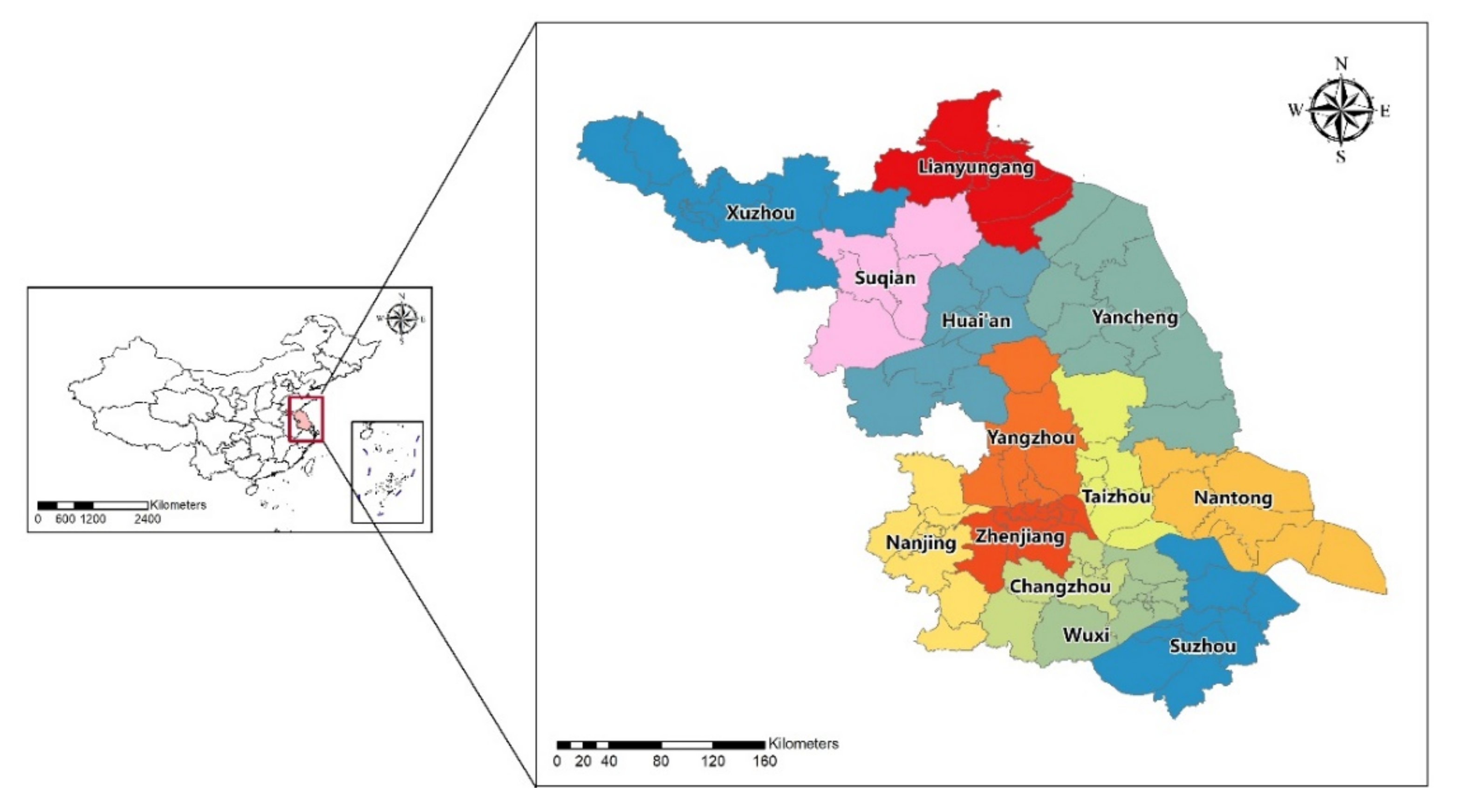
In this paper, we take counties of Jiangsu Province China (Figure 1), a typical coastal plain region, as the basic research unit. We aim to explore the unbalanced development characteristics of regional urban spatial forms. The objectives of this paper are (1) to identify the unbalanced development characteristics and compare the differences among the urban spatial expansion size, development intensity, and distribution aggregation degree; (2) to identify their different driving mechanisms by using modern spatial analysis tools and data on physical geography, economy, and society; and (3) to put forward a differentiated regional optimization adjustment strategy.

2. Methods and Data Sources

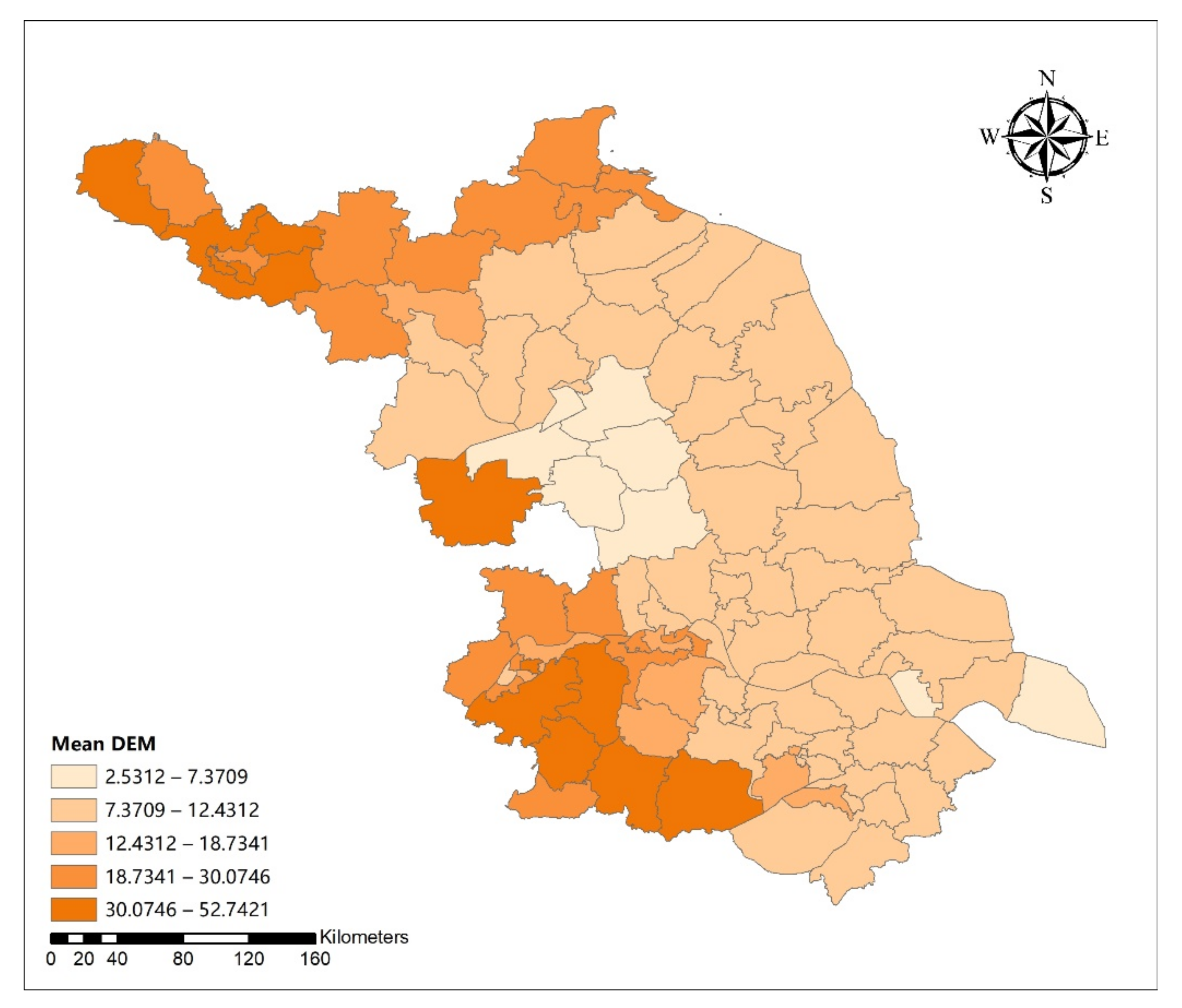
Since districts and counties have the same administrative level in China, we took the districts and counties of Jiangsu Province as the basic research unit, with a total of 99 spatial samples. Jiangsu is located in the Yangtze River Delta, with flat terrain (see Figure A23 for digital elevation model (DEM) in Appendix A), which covers an area of 107,200 km2. The latest accessible year of land use data and point of interest (POI) data is 2015, and other statistical data also has a certain lag. In order to match spatial data with social and economic data, we selected 2015 as the study year. In 2015, Jiangsu Province had a total population of 80 million, with a GDP of 7012 billion Chinese yuan (CNY). The area of the built-up area, the proportion of built-up area, and the global Moran’ I of the built-up area of each district and county were used to characterize urban spatial expansion size, development intensity, and distribution aggregation degree. First, spatial autocorrelation analysis was used to analyze the spatial distribution pattern and characteristics of urbanization in Jiangsu Province. Then, the traditional statistical methods and spatial statistical methods were combined to analyze 30 commonly considered potential driving variables related to physical geography, economy, and society [12,36]. Pearson correlation analysis was used to screen out the variables that were significantly related to the spatial pattern of urbanization. Finally, linear regression (ordinary least squares: OLS) and geographically weighted regression (GWR) were used to identify the driving variables that led to the difference in urbanization spatial form.

2.1. Data

The data used in the study were obtained from the following sources. The physical geography and remote sensing monitoring data of the status of land use in Jiangsu Province in 2015 with a resolution of 1 km comes from the Resource and Environment Science Data Center of the Chinese Academy of Sciences (http://www.resdc.cn/; accessed date: 20 March 2020). It is based on Landsat 8 remotely sensed images and was generated by human visual interpretation. The social and economic data came from the 2015 “Statistical Yearbook of Jiangsu Province” (http://stats.jiangsu.gov.cn/2015/indexc.htm; accessed date: 20 March 2020) and the statistical yearbook of each city. The population data came from the sixth national census of the National Bureau of Statistics (http://www.stats.gov.cn/tjsj/pcsj/rkpc/6rp/indexch.htm; accessed date: 20 March 2020). The point of interest (POI) data came from the 2015 Gaode map. These data are listed in Table 1. We divided potential influencing variables of urban spatial form into three types. The variables of physical geography were mainly dependent on the natural background environmental conditions, related to geographical location and formed naturally; the economic variables were related to economic income and industrial development; the societal variables were related to social and historical development, influenced by human beings and driven by human development needs. This categorization and choice of variables reflect common practice among researchers working on related studies [19,20,21,22,23,24,25,28,36].
We extracted the urban land from the remote sensing monitoring data of Jiangsu Province in 2015 as the built-up area. The value of built-up area and non-built-up area was recorded as 1 and 0, respectively. First, we calculated the area of the built-up area, the proportion of the built-up area, and the global Moran’s I (see Section 2.1) of the built-up area within each district or county. We used these three indicators to represent urban spatial expansion size, development intensity, and distribution aggregation degree, respectively.

2.2. Methods

In this section, we present the statistical methods used in this paper for correlation in and regression analysis. We first summarize the conventional, non-spatial approach (correlation, regression) and then the associated spatial method (Moran’s I, GWR) and explain their relevance in this study. We also provide references that readers can consult for further details on the methods and applications.

2.2.1. Pearson Correlation Analysis

The Pearson product moment correlation coefficient [37,38] was used to evaluate the linear correlation between two continuous variables.
Pearson   r = i x i x ¯ y i y ¯ i x i x ¯ 2 i y i y ¯ 2
where x ¯ and y ¯ are the sample mean values of two continuous variables x and y , respectively, and the value range of r is in [–1,1]. If r > 0, it means that the two variables are positively correlated, if r   <   0 , then the two variables are negatively correlated, and if r = 0, it means that there is no linear correlation between the two variables. Since r is estimated from a sample, a hypothesis test is used to evaluate whether the true correlation, ρ, is significantly different from zero.
As shown in Table 1, 30 potential variables that might have an impact on the regional urban spatial form were selected. We then performed Pearson correlation analysis in SPSS 24.0 to quantify the relationship between the three urban metrics and the 30 potential driving variables. The units being evaluated were the districts and counties of Jiangsu province.

2.2.2. Spatial Autocorrelation Analysis

Spatial autocorrelation is used to quantify the association between the attribute values of nearby units [39]. In this study, the units were the counties and districts of Jiangsu Province. Positive spatial autocorrelation indicates that counties with similar attribute values are located close to each other and negative spatial autocorrelation indicates that counties with different attribute values are located close to each other. If the spatial autocorrelation is close to zero, then there is no spatial association. As with Pearson’s correlation, this can be assessed using a hypothesis test. Spatial autocorrelation can be evaluated using the Moran’ I index [31,39,40]. The value of I is between [−1,1], −1 indicates perfect negative autocorrelation, and 1 indicates perfect positive autocorrelation, 0 means no spatial autocorrelation. The formula for the global Moran’ I is shown below.
I = N i j w i j i j w i j x ( s i x ¯ ) x j x ¯ i ( x i x ¯ ) 2
where s indicates location and i , j identify specific spatial units; w i j is the spatial connectivity matrix. If two geographic units are adjacent, the value is 1, and if the two geographic units are not adjacent, the value is 0; x i and x ¯ are the value of the attribute in the i -th geographic unit and the mean value of the study area; N is the total number of geographic units. The formulation is similar to Pearson’s r ; however, we only consider one variable rather than two and evaluate how observations of that variable are related to observations of the same variable at adjacent locations.
There is also a local version of Moran’s I, which calculates the statistic at location s i
I s i = N x i x ¯ j w i j x j x ¯ i ( x i x ¯ ) 2
Global statistics evaluate the spatial autocorrelation over the whole study area. They assume that the autocorrelation is constant over the study area but, in reality, it can vary in space. Local statistics calculate the spatial autocorrelation around a specific spatial unit [31,32,41]. These local statistics are called local indicators of spatial association (LISA) [41] and they have been used in both environmental and social-science studies [27,31,32] to evaluate local patterns. Here, we used ArcGIS 10.6 to calculate the local Moran’s I, and identify high-value clusters (H-H), low-value clusters (L-L), outliers with high values mainly surrounded by low values (H-L), and outliers with low values mainly surrounded by high values (L-H). We implemented spatial autocorrelation analysis in software GeoDa [42].
We used the global Moran’s I, calculated for the built-up area within each county or district, to define the urban aggregation degree.

2.2.3. Linear Regression (Ordinary Least Squares Regression: OLS)

Linear regression analysis is often used to study the relationship between the variable of interest (the response variable) and one or more covariates. It can also be used for prediction [37,43]. It can be expressed as:
y i = β 0 + k = 1 p β k x k i   + ε i ,
where y i is the value of the response variable associated with the i th observation and β 0 is the constant (intercept) term; β k   is the regression coefficient, and ε i is the residual, which represents the difference between the fitted value and the true value. In the most simple case, p = 1 and there is only one covariate, x i . In this paper, we evaluated multiple covariates (Table 1) for predicting the three characteristics of urban form: urban spatial expansion size, urban spatial development intensity, and urban spatial distribution. The analysis was restricted to linear regression. OLS refers to the method used to estimate the regression coefficients using the data. It is based on minimizing the sum of squares of the residuals (hence “least squares”) [43]. We used IBM SPSS statistic 24.0 to establish an OLS regression equation with variables that were significantly related to urban spatial expansion size, development intensity, and distribution aggregation degree and used the stepwise method to automatically eliminate variables with strong collinearity to obtain the final OLS regression equation.

2.2.4. Geographically Weighted Regression

Geographically weighted regression (GWR) [44] extends the linear regression model and uses the local weighted least square method to calculate the regression coefficient. In other words, the weight is determined according to the Euclidean distance between the spatial position of the estimated point and the spatial position of other observation points, so that the regression coefficient of the model is no longer a single global value, but can vary in geographic space [34]. The estimated parameter values at different geographical locations describe the spatially varying nature of the relationship between y and x . The structure of the model is as follows:
y s i = β 0 s i + k β k s i x k s i + ε i
where y s i is the response variable of the i-th sample at location s i ; x k s i is the value of the k -th covariate at the i -th location; ( s i ) is the coordinate of the i -th point; β k s i is the local regression coefficient at s i ; and ε i is the residual. The key difference between GWR and OLS is that the regression coefficients can vary in space. Hence, it is necessary to indicate the location ( s i ) of each observation and associate regression coefficient (compare Equations (4) and (5)).
GWR has been used to model spatially varying relationships in both the social [44] and environmental sciences [34]. This gives more flexibility compared to linear regression (OLS) because the regression coefficients ( β k in Equation (5)) can vary in space. Exploring the spatial variability in the relationship between the response variable and covariates can give more insights into the process [33] Note that GWR does not automatically lead to an improvement compared to OLS. This needs to be evaluated.
We used covariates from the OLS model and put them into the GWR model to explore the spatial structure in the driving forces of regional imbalance in urban spatial form. GWR was implemented in ArcGIS 10.6.
We computed the following statistics for the OLS and GWR mode: the standard error of the residuals, σ ^ ; the coefficient of determination, R2; the adjusted-R2 and the adjusted Akaike information criterion (AICc) [37]. The standard error of the residuals quantifies the variability of the residuals around the fitted regression line. The coefficient of determination quantifies the proportion of the variability in the response variable that is explained by the model and take as a value between 0 and 1 (larger is better). The adjusted-R2 is the R2 adjusted for a number of covariates. Adding covariates to a linear regression model will not reduce the R2, but does increase the model complexity. Hence, the adjusted-R2 supports evaluating whether adding a covariate is sufficiently useful to justify the increase in model complexity. AICc is commonly used to compare models. It gives a trade-off between goodness-of-fit and model complexity. A lower AICc indicates a better model.

3. Results

3.1. Spatial Pattern and Spatial Autocorrelation of Urban Form in Jiangsu Province

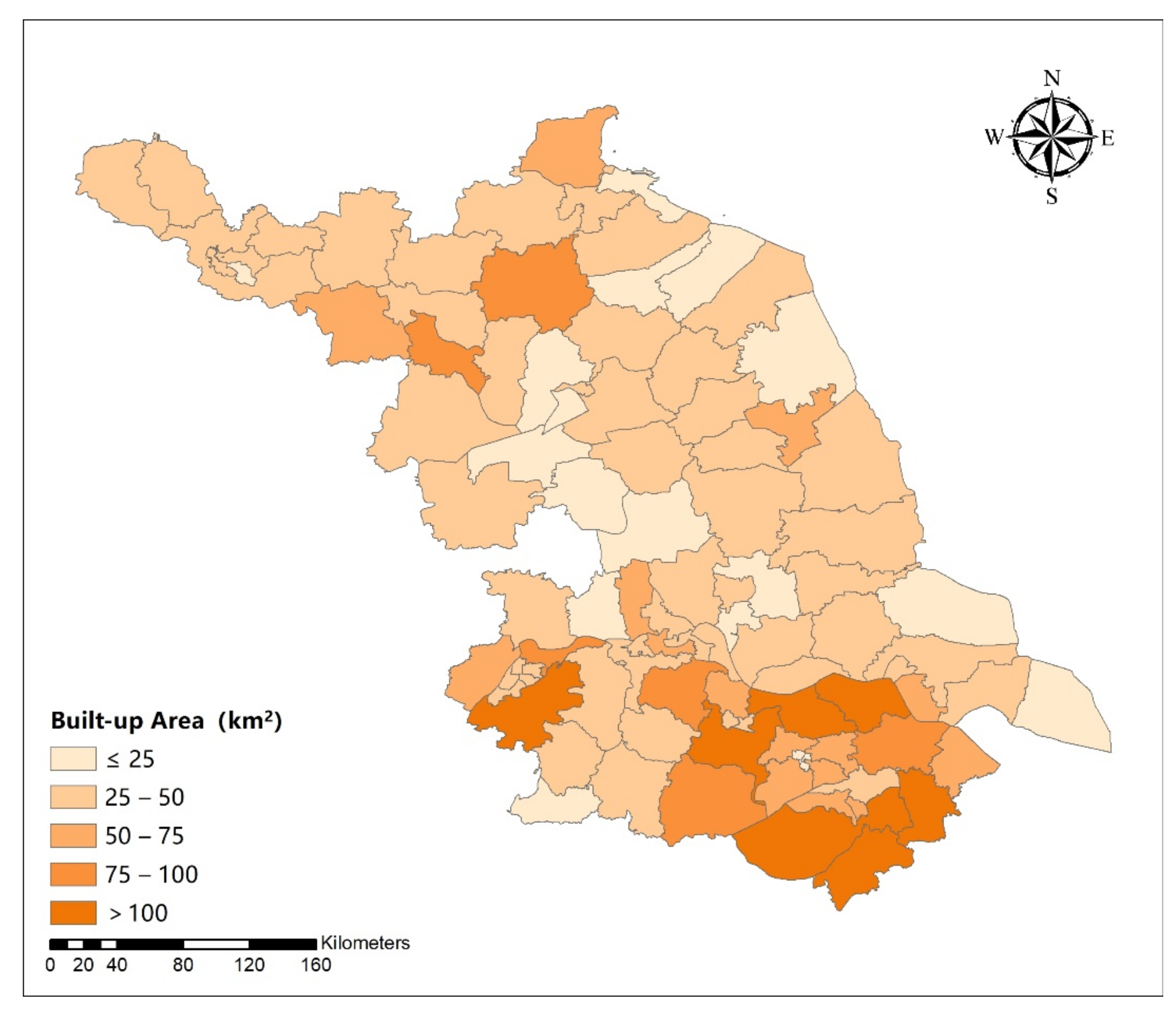
The area of all districts and counties in Jiangsu Province was between 11 and 142 km2 (Figure 2). Figure 2 shows that the districts and counties with larger spatial expansion sizes were mainly distributed in southern Jiangsu. Most districts and counties (52 out of 99) had a built-up area in the range 25–50 km2. Most (87%) of the districts and counties’ size were less than 75 km2. As shown in Figure 3, the proportion of the built-up area in the districts and counties in Jiangsu Province varied greatly, ranging from 0.0042 to 0.7286. The counties with urban development intensity >0.05 were mainly concentrated in southern Jiangsu. Most (59%) districts and counties had a development intensity ≤0.05. The urban aggregation degree (Figure 4) of built-up area did not show a distinct pattern. The values ranged from 0.14 to 0.71, with the largest values in the south and the north-east.
As shown in Table 2, the global Moran’ I index of urban spatial expansion size, development intensity, and distribution aggregation degree were 0.212, 0.394, and 0.076, respectively, and all, except distribution aggregation degree, were significantly different from zero. These positive spatial correlations show that the urban size and development intensity were spatially correlated, hence the districts and counties with similar urban expansion size and development intensity tend to be clustered. For distribution aggregation degree, the p-value is relatively large (0.081) indicating that Moran’ I index of urban spatial distribution failed the significance test. This suggested that there was no clear evidence of global spatial autocorrelation and no agglomeration phenomenon in the urban aggregation degree of districts and counties in Jiangsu Province.
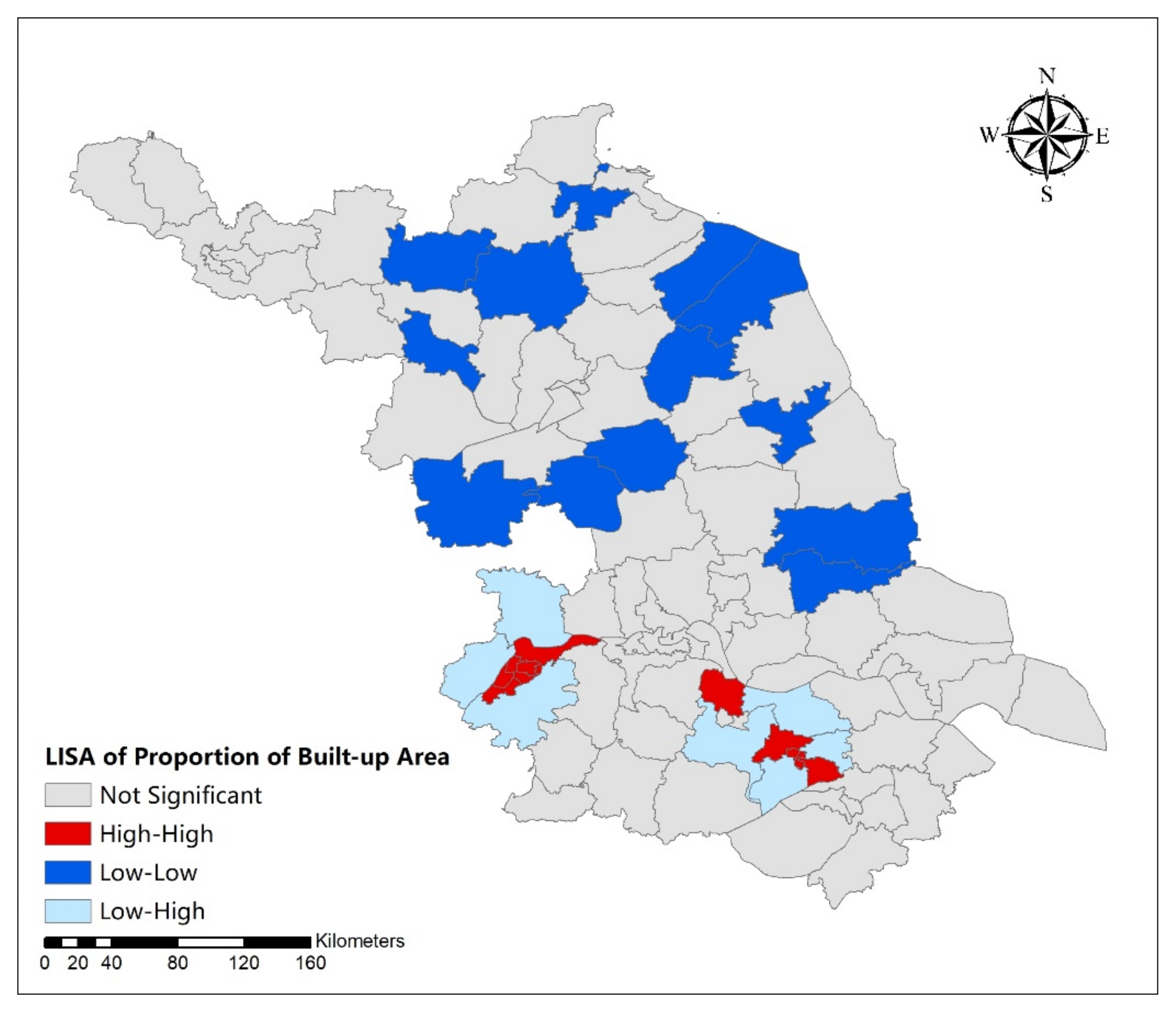
The LISA (Local Moran’s I) cluster map of local hot spots is shown in Figure 5 and Figure 6. For the urban expansion size (Figure 5), the districts and counties with high-high aggregation all appeared in southern Jiangsu; the districts and counties with high-low or low-high aggregation appeared in central Jiangsu; and the districts and counties with low-low aggregation appeared in northern Jiangsu. This indicated that the built-up areas were generally more clustered in southern Jiangsu than those in northern Jiangsu. Central Jiangsu acted like a transition region. As for urban development intensity, there were three types of aggregation in Jiangsu: high-high, low-low, and low-high. Both the districts and counties with low-high and high-high aggregation areas were distributed in the center and south of Jiangsu Province. The districts and counties with low-low aggregation were all in the middle and north of Jiangsu Province. This indicates a regional imbalance in the urban development intensity in Jiangsu Province.

3.2. Correlation Analysis of Covariates of Urban Spatial Form in Jiangsu Province

As shown in Table 3, among the 30 potential variables, there were 23 that were significantly related to the urban expansion size, of which 20 variables were positively correlated. The three variables with the largest correlation coefficients were GDP, output of the secondary industry, and total numbers of POIs. On the other hand, the proportion of the over 60-year-old population, proportion of primary industrial output value, and the distance to Shanghai were negatively correlated to the urban spatial expansion size. Meanwhile, there were 19 variables that were significantly related to the urban development intensity, 12 of which were positively correlated. The variables with the largest correlation coefficients were road density, urban population density, and urban population ratio. Seven variables were negatively correlated and the three variables with the largest correlation coefficient were the proportion of the output value of the secondary industry, the area of the districts and counties, and rural population. There were 17 variables significantly correlated with the urban distribution aggregation degree, 10 of which were positively correlated. The variables with the largest correlation coefficient were proportion of urban population, the density of urban population, and the density of roads. The three variables with the largest negative correlation coefficient were the output value of the primary industry, area of districts and counties, and rural population.
The urban spatial expansion size had a strong correlation with the size indicators of social and economic development, while the urban spatial development intensity and the spatial distribution aggregation degree had a strong correlation with indicators of density or proportion such as road density, urban population density, and urban population proportion.

3.3. Driving Force Analysis of Urban Spatial Form in Jiangsu Province

3.3.1. Driving Force Analysis of Urban Spatial Expansion Size

Compared to the OLS model parameters of influencing variables of urban spatial expansion size, GWR model almost has the same parameters (Table 4). According to the results of OLS (Table 5), there were five variables affecting the urban spatial expansion size. The standardized regression coefficient reflected the degree of influence without dimension, which was in the order of output of the secondary industry, total number of POI, proportion of population over 60 years old, income of national and provincial development zones, and total export–import volume. Most of the variables had a positive relationship with the urban spatial size except the influence of proportion of population over 60 years old and total export–import volume. Therefore, the higher the secondary output value, the more POI’s, the larger the income of the development zone, the less aging population, and the lower the total import and export volume, the larger the built-up area.
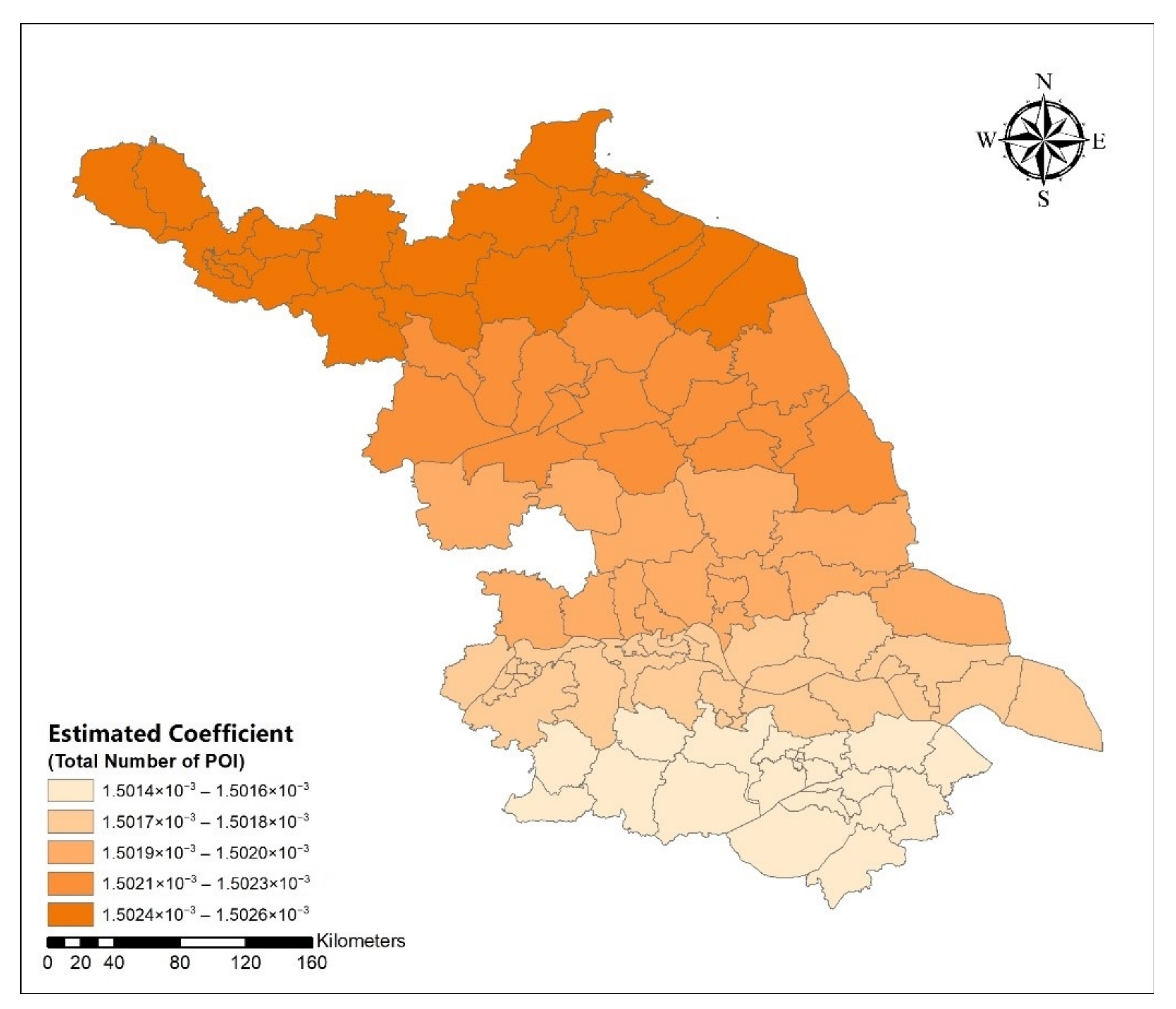
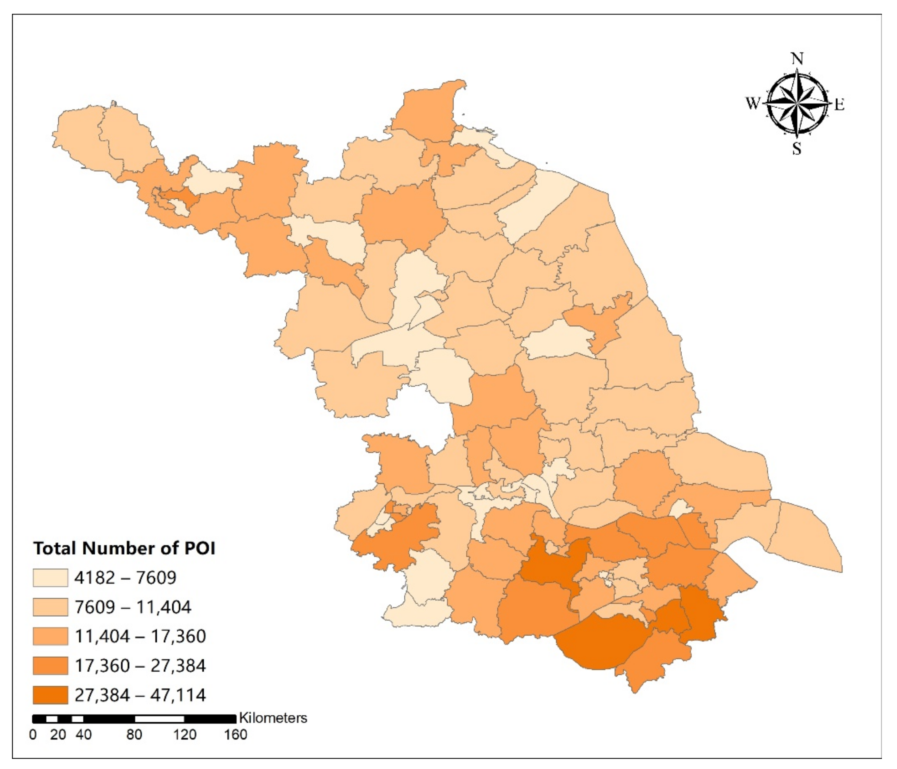
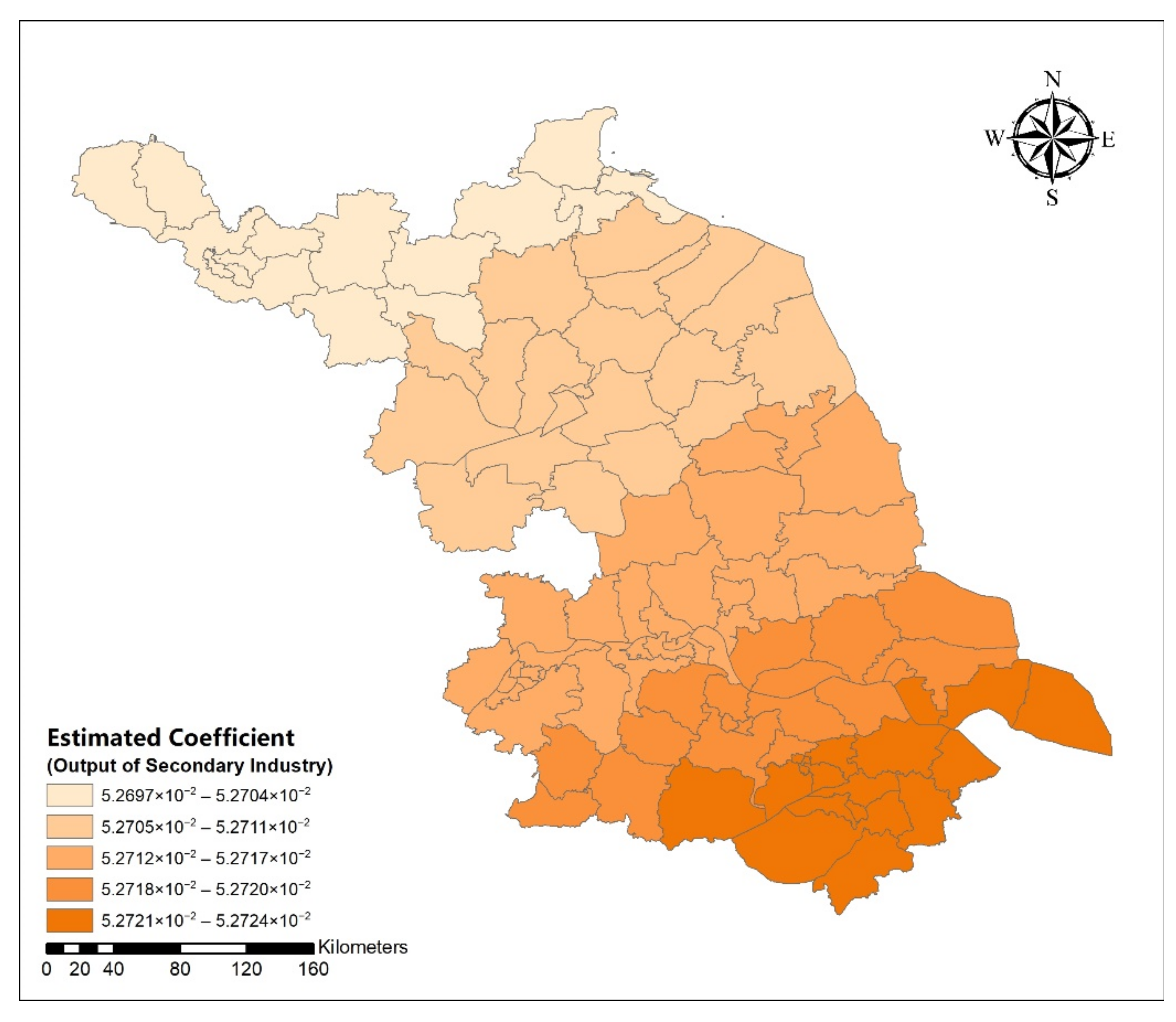
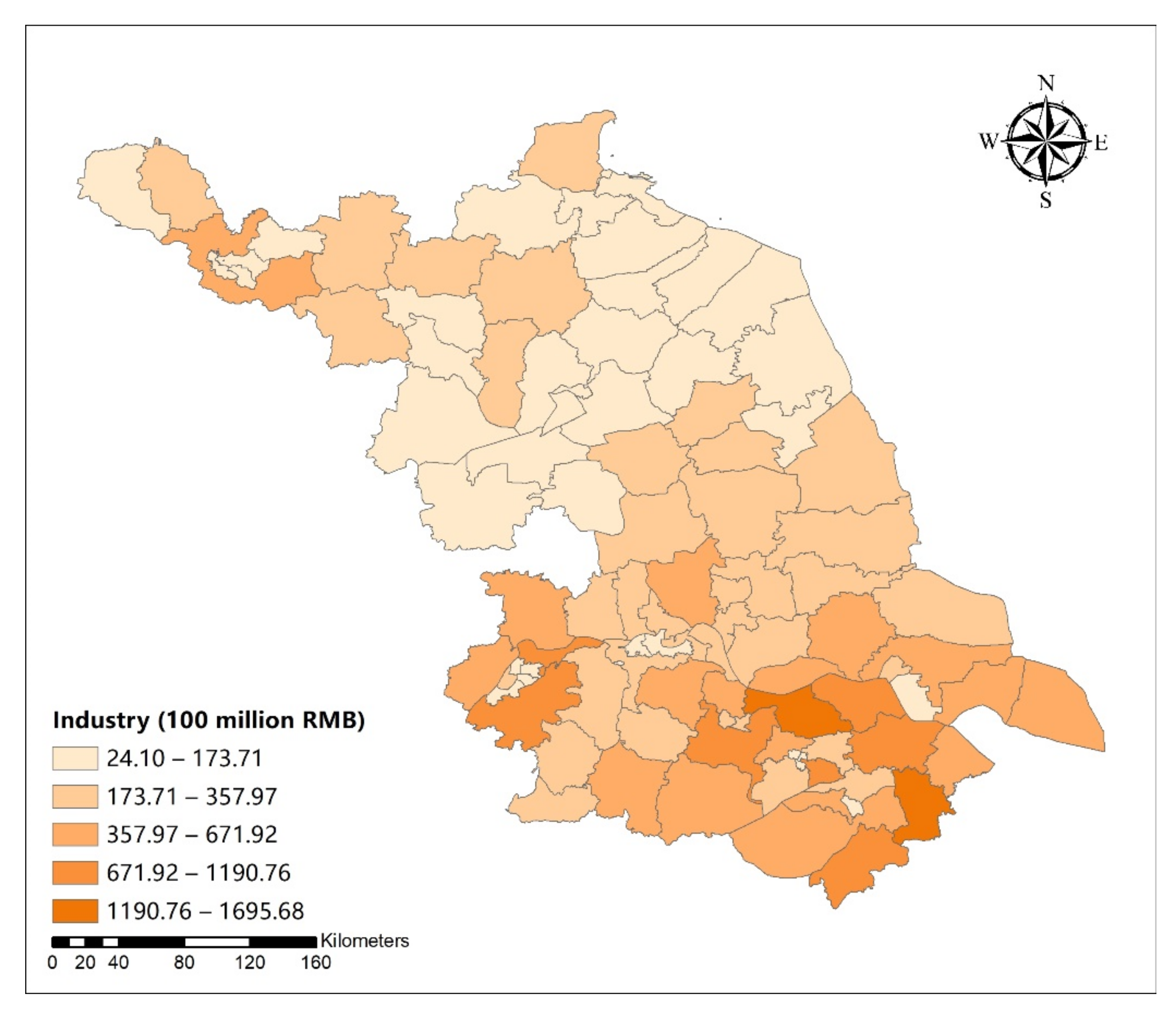
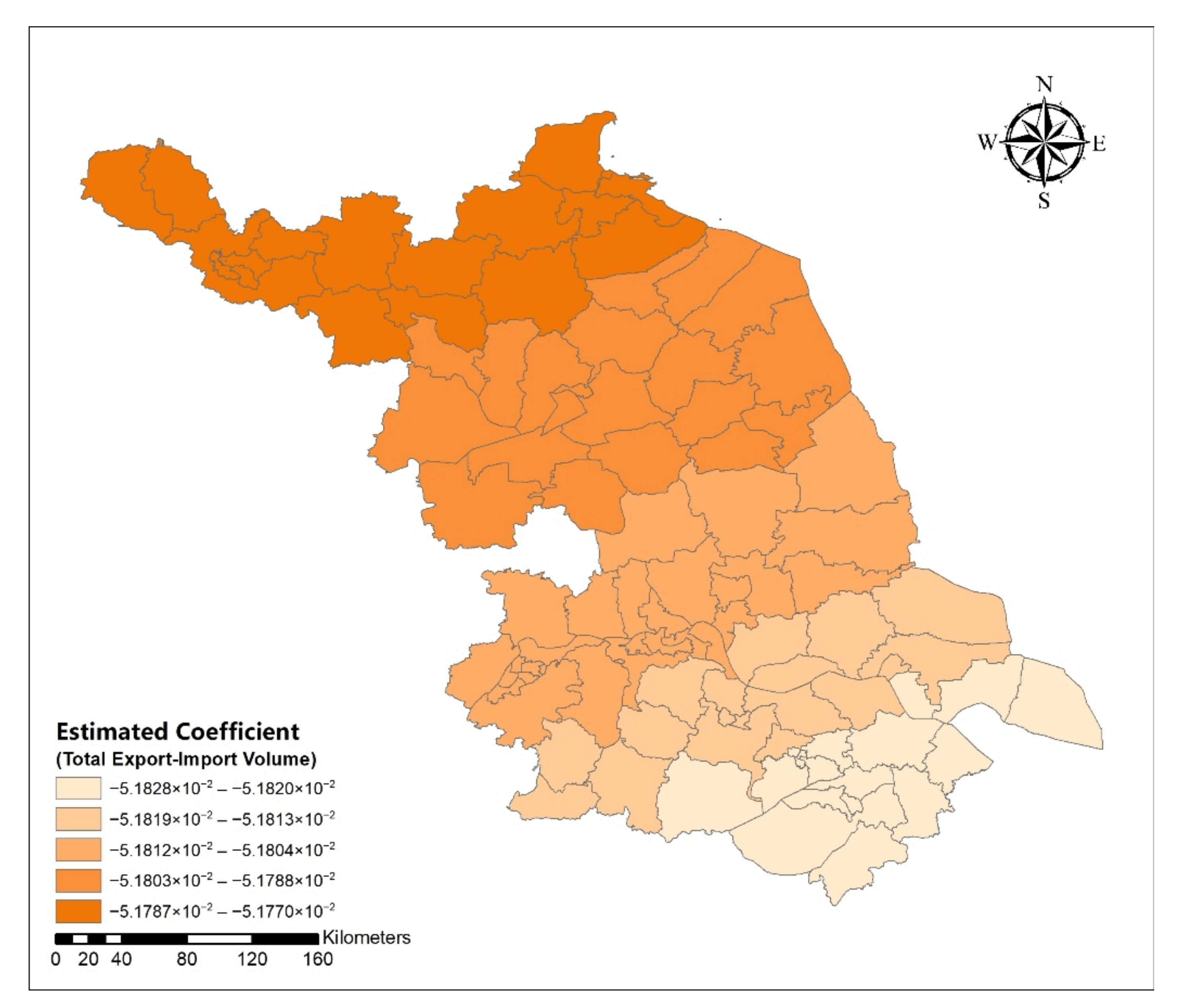
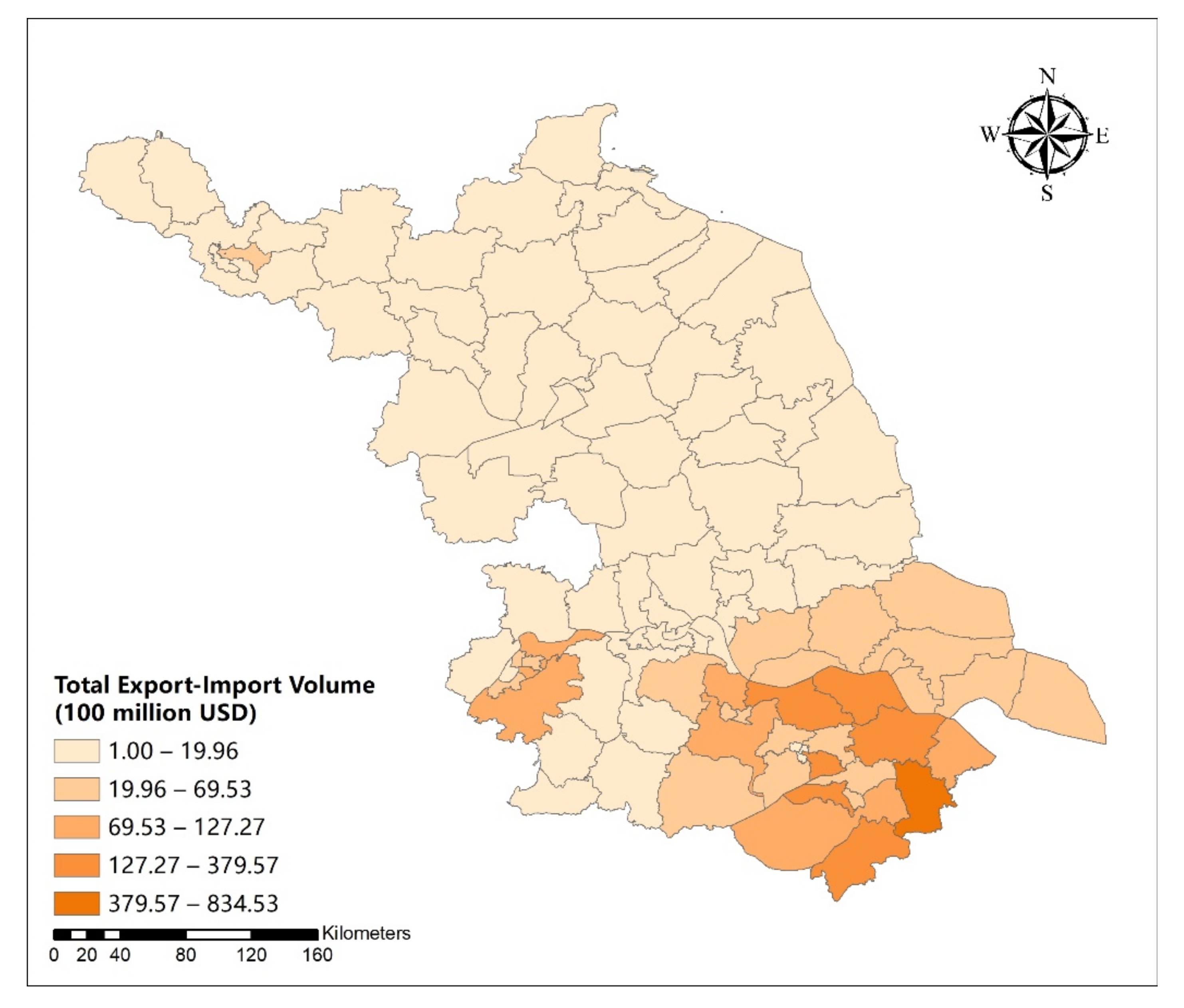
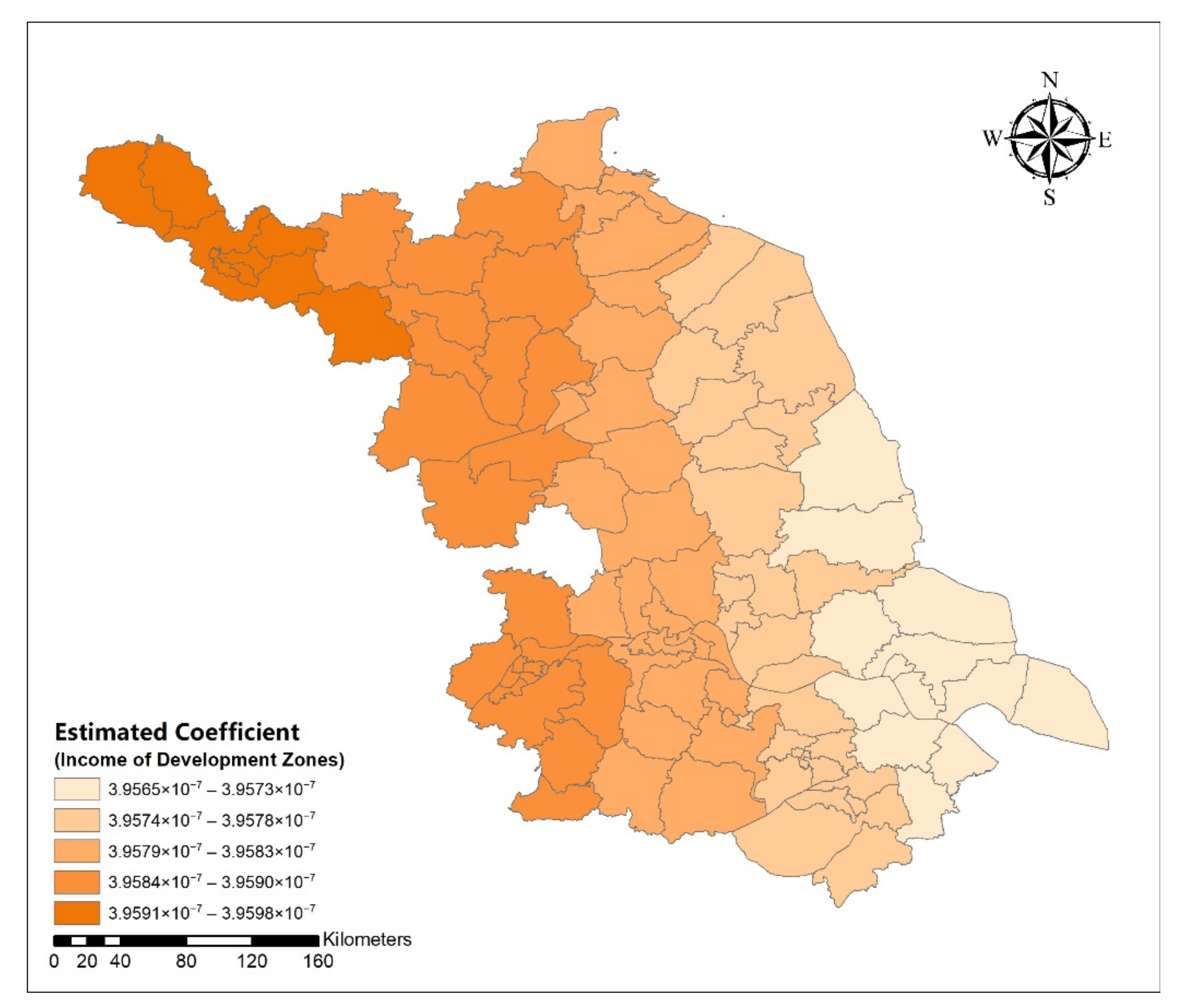
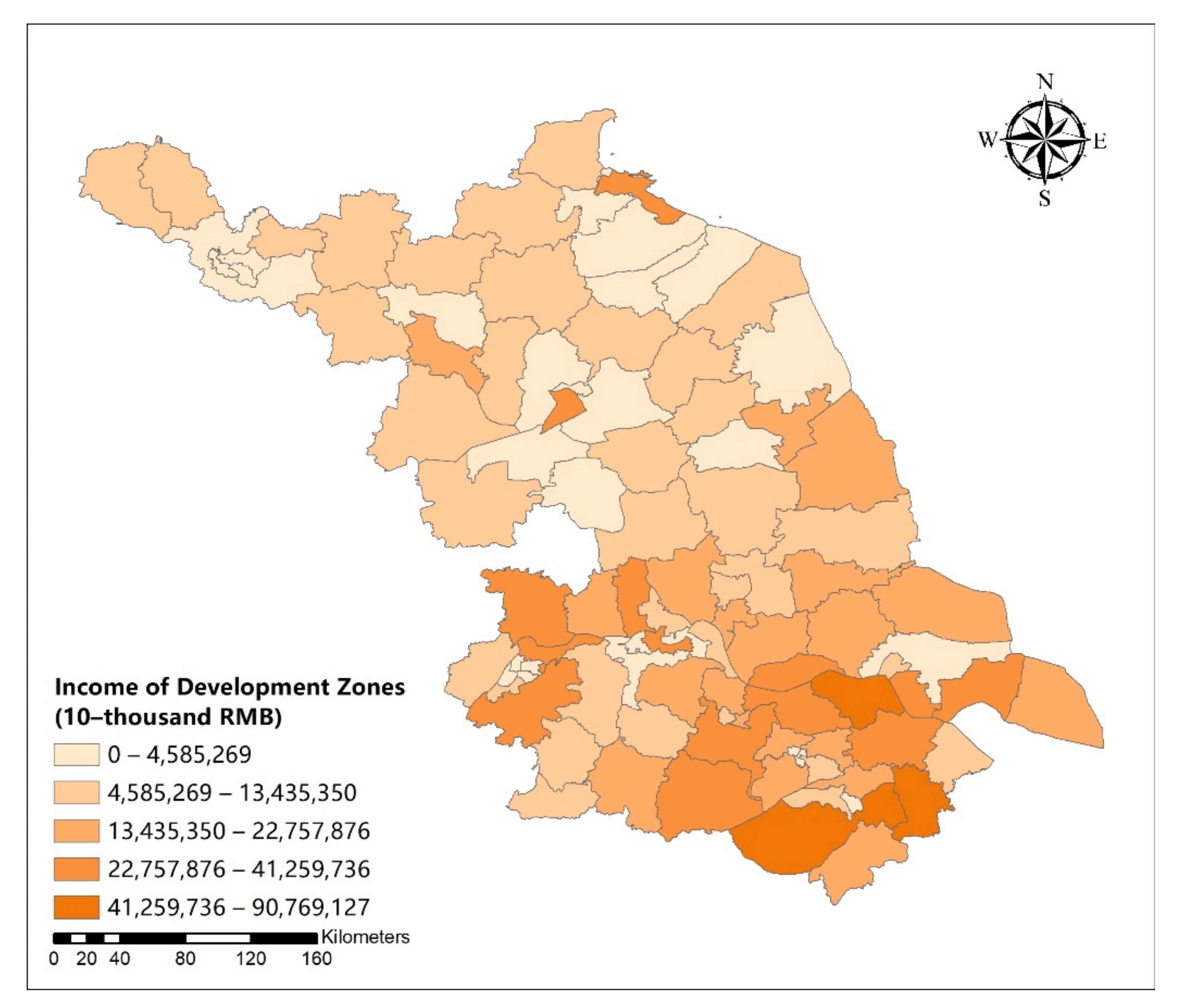
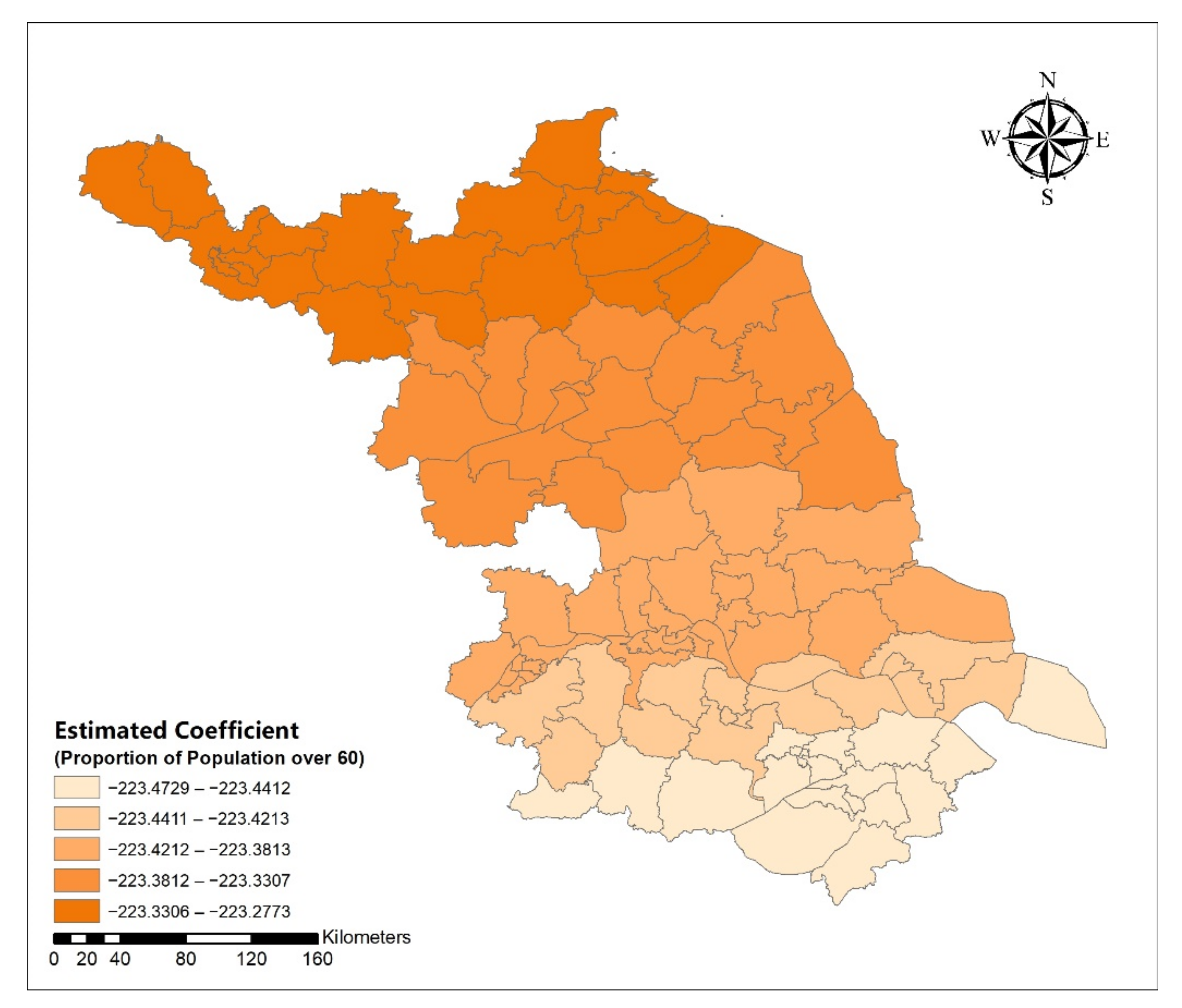
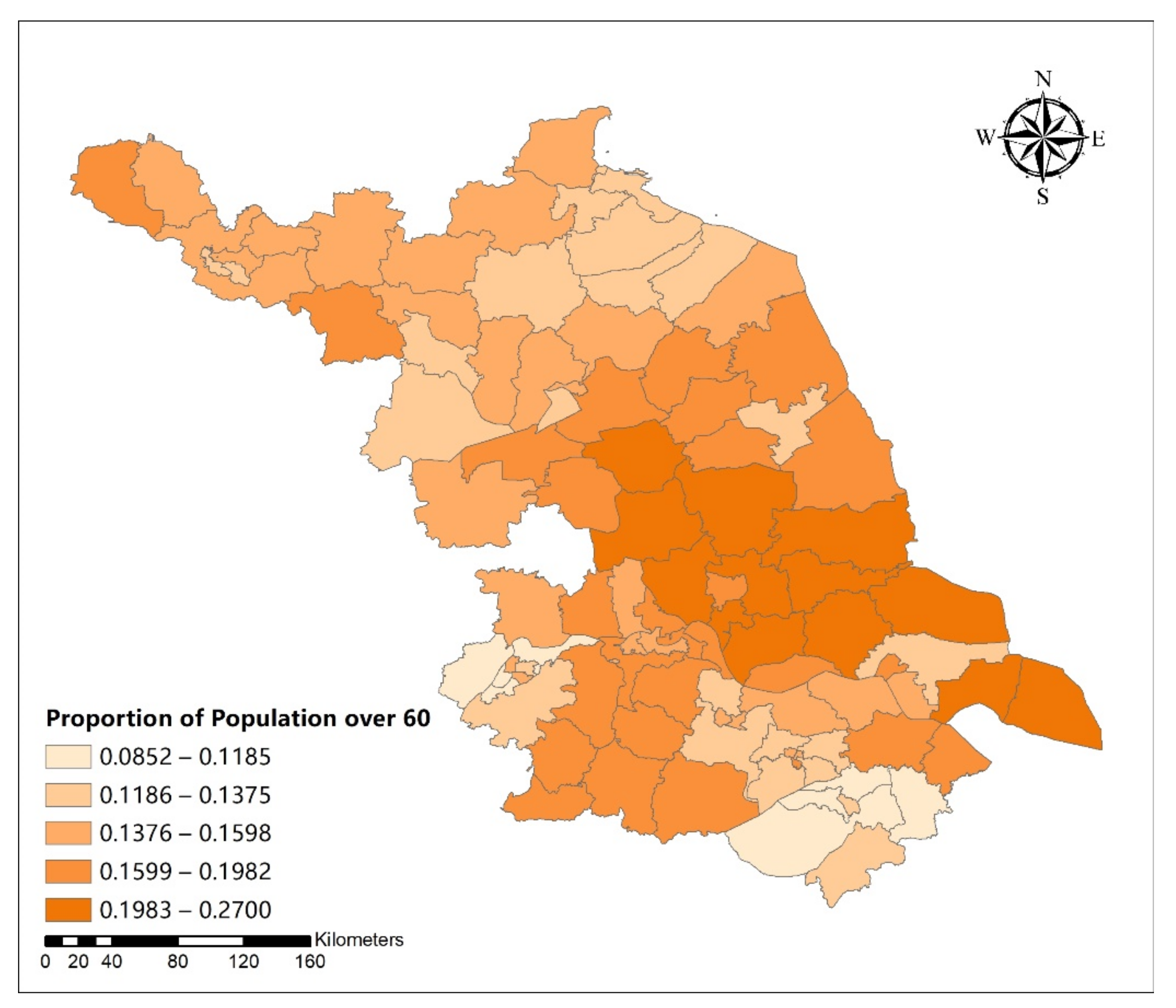
Table 6 shows the estimated GWR coefficients. From Appendix A Figure A1, Figure A2, Figure A3, Figure A4, Figure A5, Figure A6, Figure A7, Figure A8, Figure A9 and Figure A10, we could see the spatial differences between the estimated coefficient and the influencing variables. The spatial influence degree of proportion of population over 60 years old, total number of POIs, and total import and export amount in space showed a decreasing trend from north to south Jiangsu, while the influence degree of the output value of secondary industry to the built-up area was opposite. In addition, the impact of income of the development zone showed a trend that decreased from west to east.
The statistics given in Table 4 show that the σ ^ , R2, and adjusted R2 were similar for OLS and GWR. The AICc was larger for GWR than for OLS, reflecting the greater model complexity. We concluded that there is no benefit to using GWR rather than OLS. Put another way, the variability in the urban spatial expansion size is sufficiently explained by OLS without needing to allow the regression coefficients to vary in space. This allows a simpler interpretation of the model results.

3.3.2. Driving Force Analysis of Urban Development Intensity

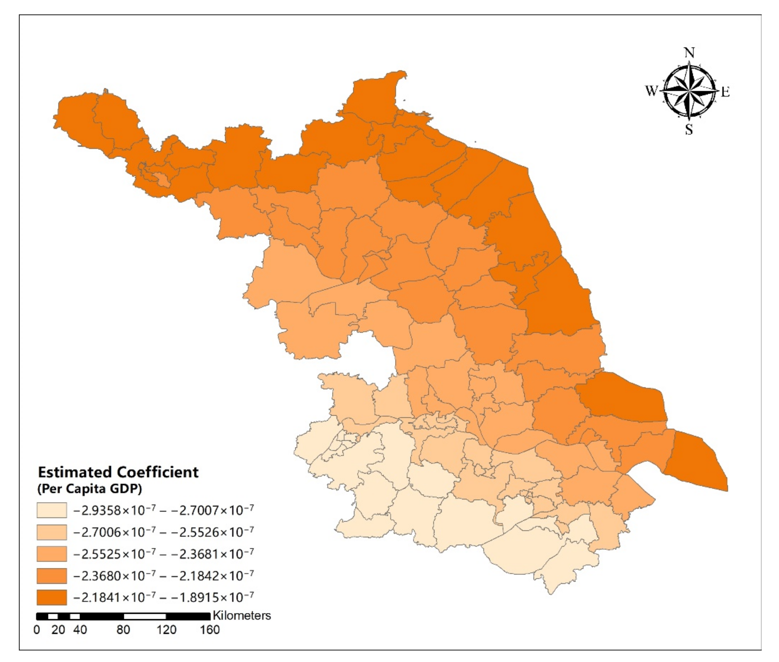
Compared to the OLS model parameters of influencing variables of urban development intensive, GWR model has higher R2 and R2-adjusted value (Table 7). The results of OLS (Table 8) showed that the four main variables influencing urban development were road density, urban population density, per capita GDP, and distance to Shanghai. The standardized coefficient for the absolute value of road density was the largest, followed by urban population density, per capita GDP, and the distance to Shanghai, while the influence of per capita GDP was negative. Therefore, as road density, urban population density, and distance to Shanghai increased and per capita GDP decreased, the urban development intensity also increased.
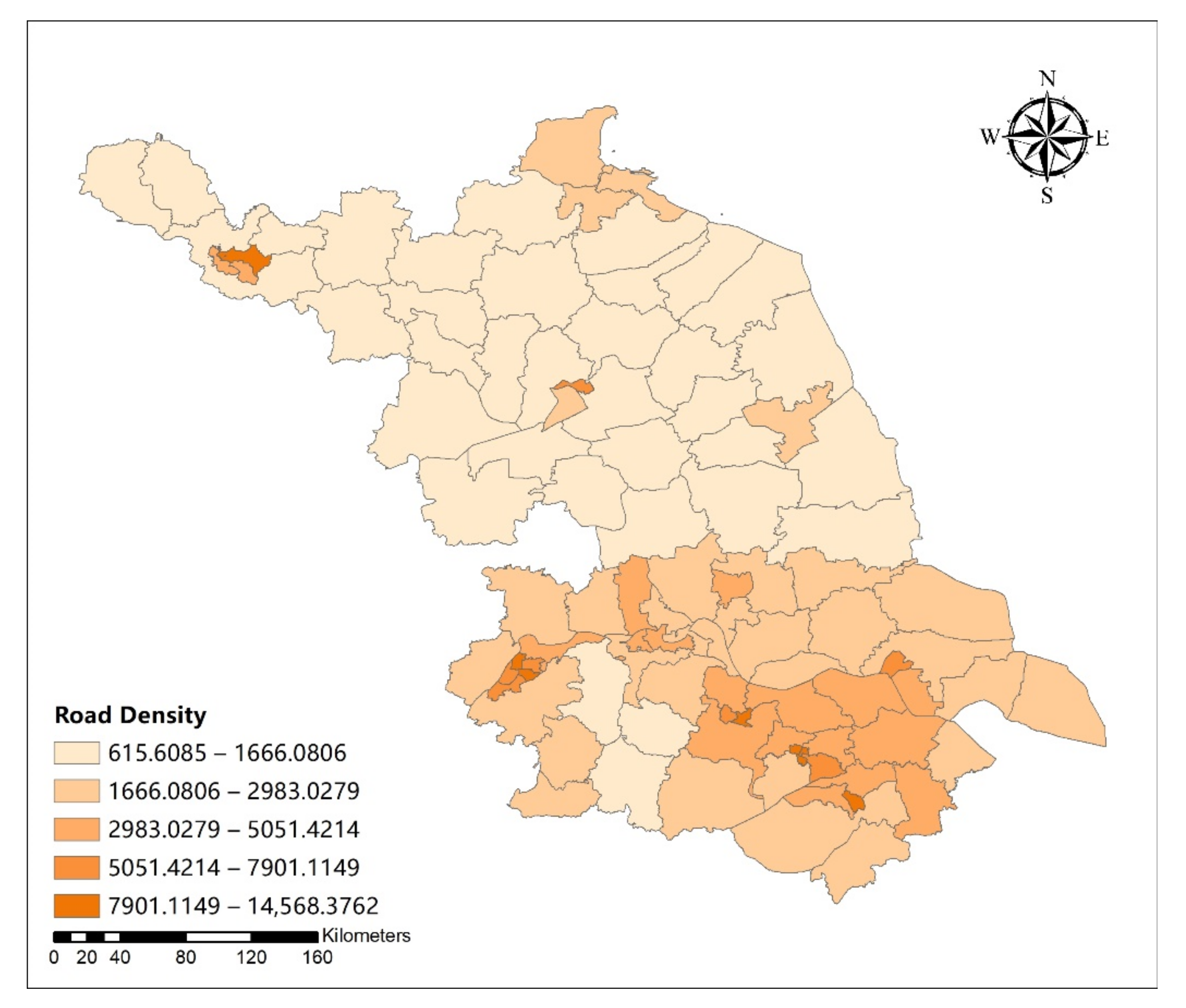
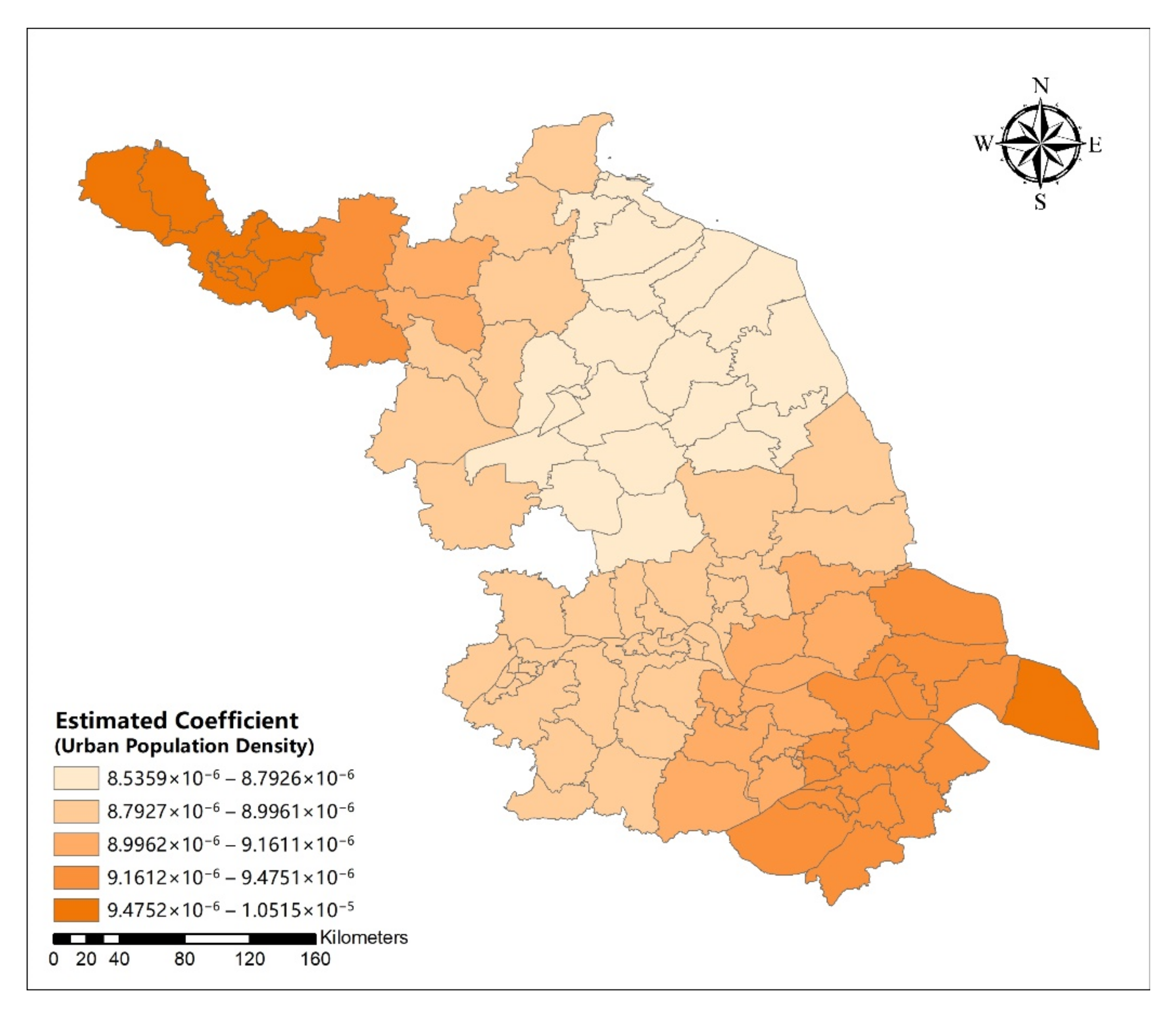
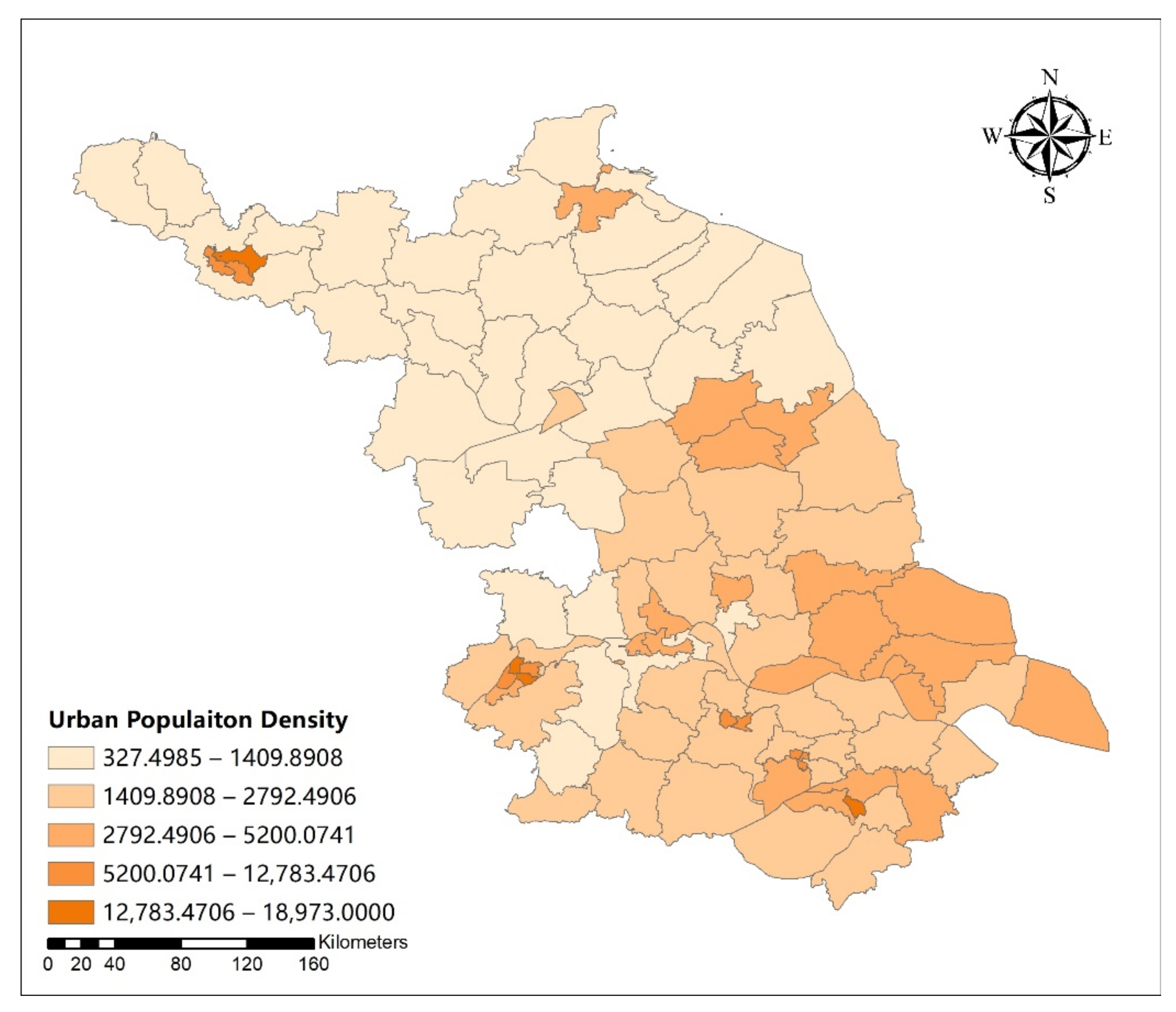
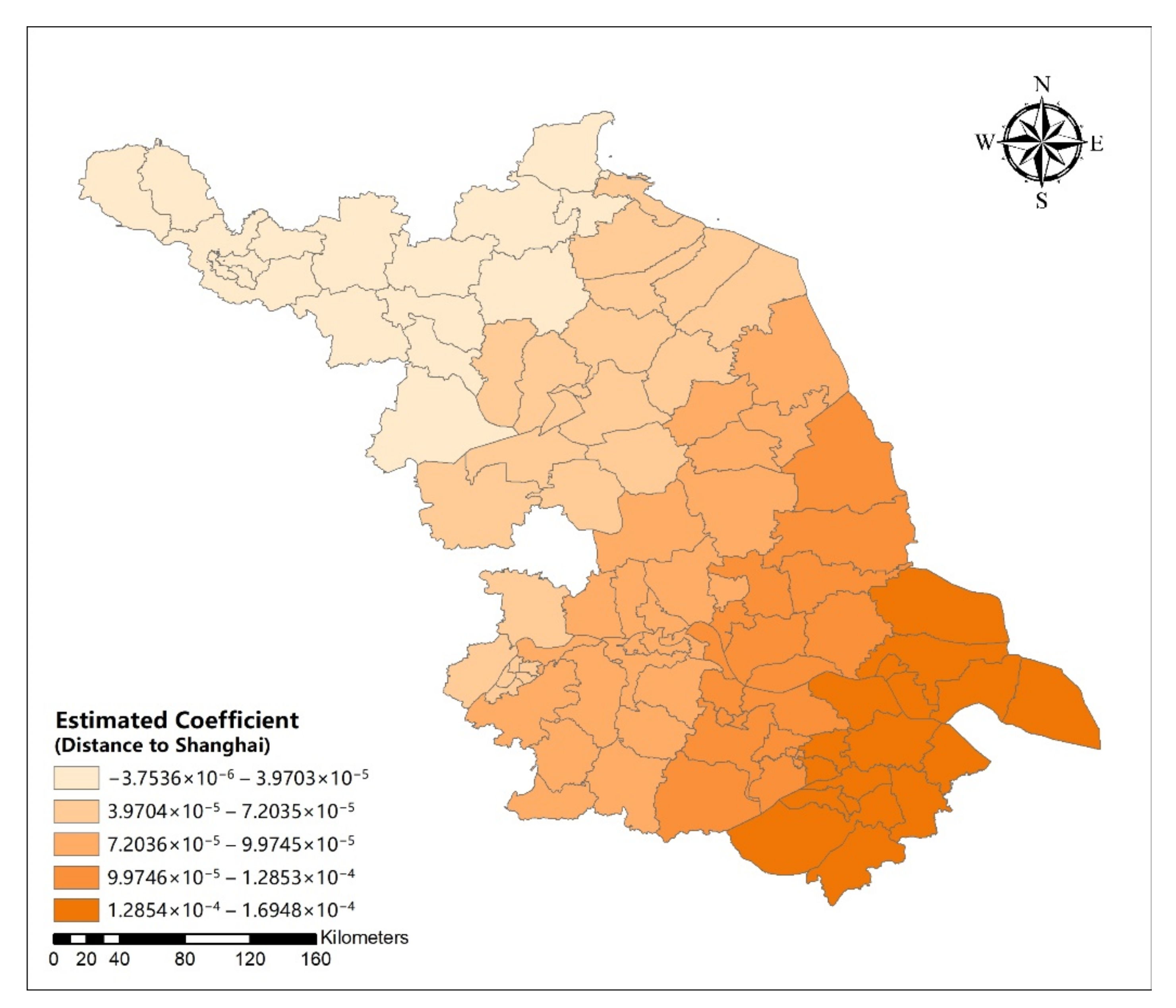
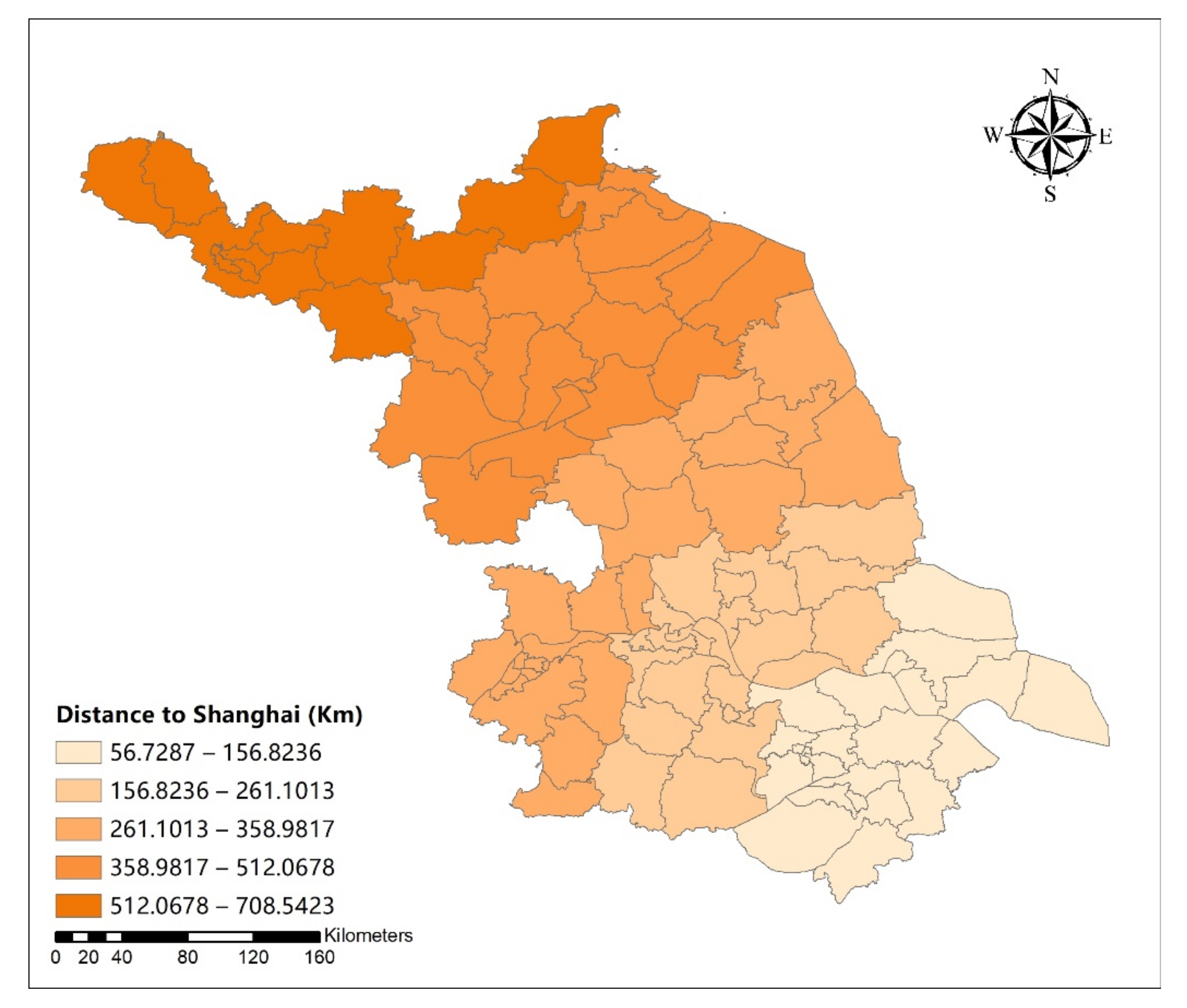
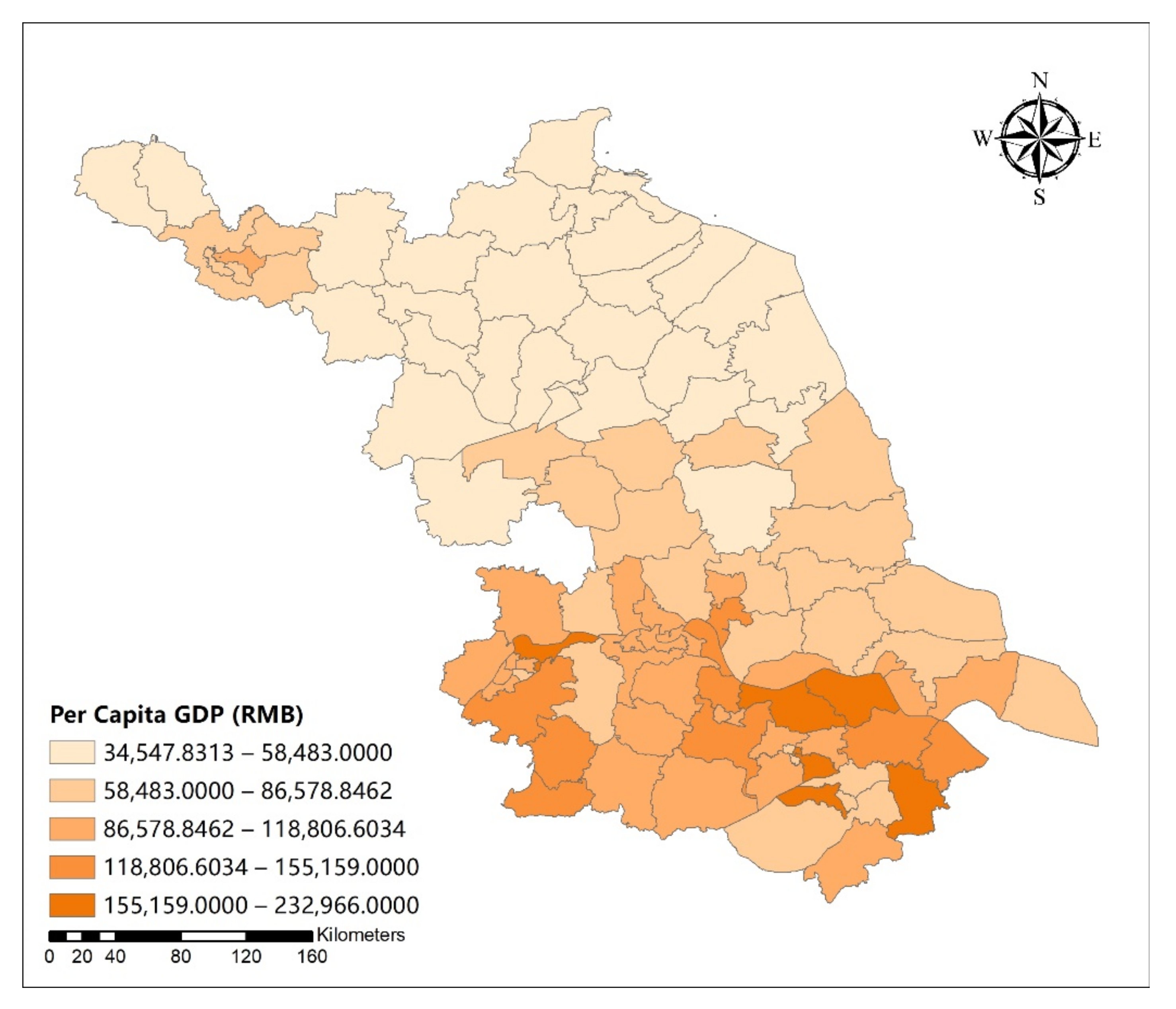
Table 9 shows the estimated GWR coefficients for influencing variables of urban development intensive. From the spatial difference of the estimated coefficients and influencing variables of the GWR model (Appendix A Figure A11, Figure A12, Figure A13, Figure A14, Figure A15, Figure A16, Figure A17 and Figure A18), the estimated coefficients of road density and distance to Shanghai showed an increasing trend in space along the southeast direction. The urban population density was the smallest in central Jiangsu, increasing along the northwest and southeast directions. Meanwhile, the per capita GDP was increasing along the northeast direction.
The model statistics are given in Table 7. These were almost identical for OLS and GLS and indicate that there was no benefit to choosing GWR rather than OLS. The variability in the urban development intensity attributable to these four covariates could be explained using the simpler OLS model.

3.3.3. Driving Force Analysis of Urban Distribution Aggregation Degree

Compared to the OLS model parameters of influencing variables of urban distribution aggregation degree, GWR model almost has the same parameters (Table 10). The results of the OLS and GWR models (Table 11 and Table 12) showed that there were two variables, terrain undulation and the proportion of urban population, affecting the urban distribution aggregation degree. The terrain undulation had a greater effect. Therefore, the flatter the terrain and the higher the population urbanization rate, the greater the distribution aggregation degree of built-up areas in the districts and counties.
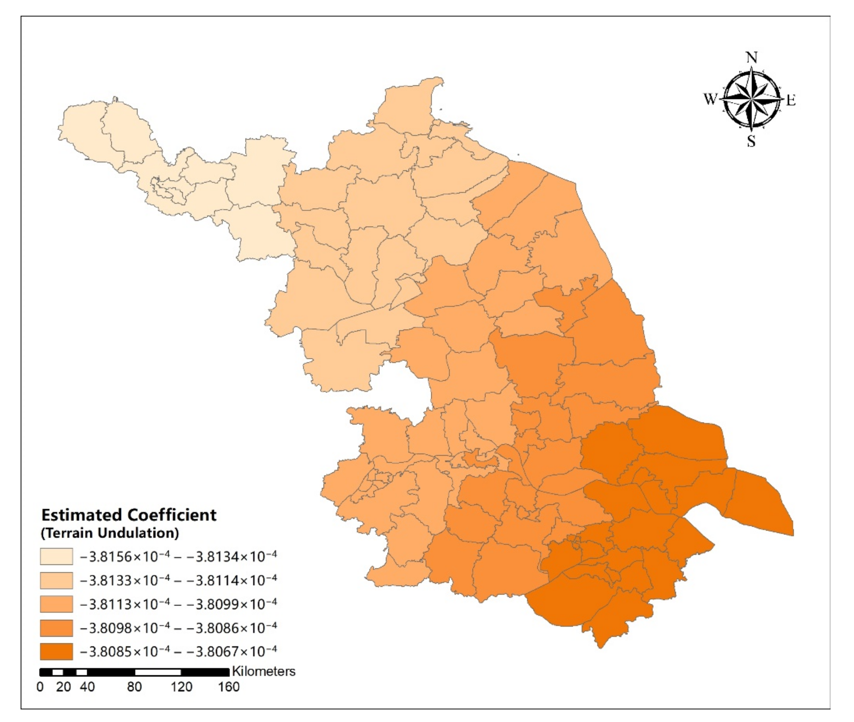
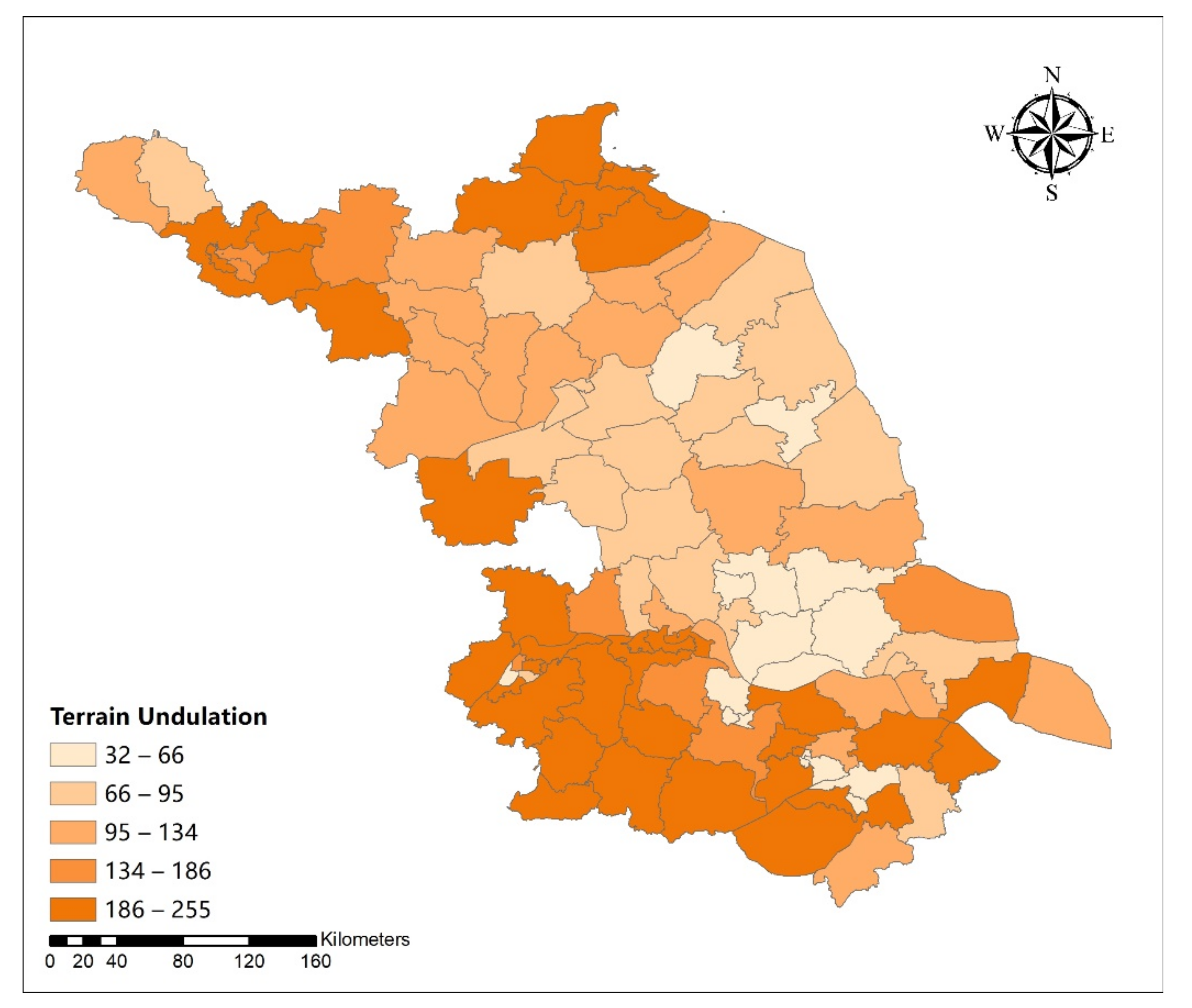
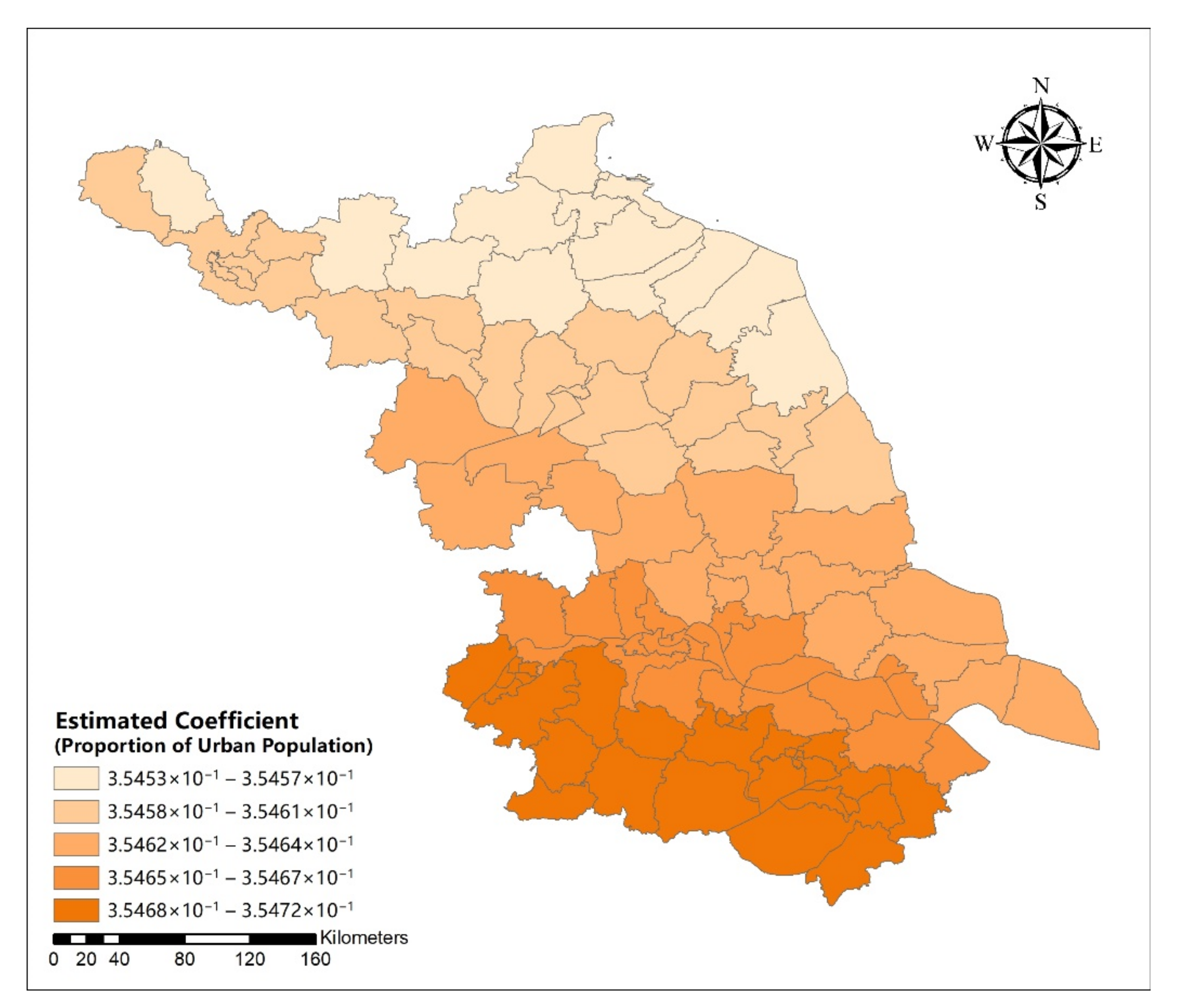
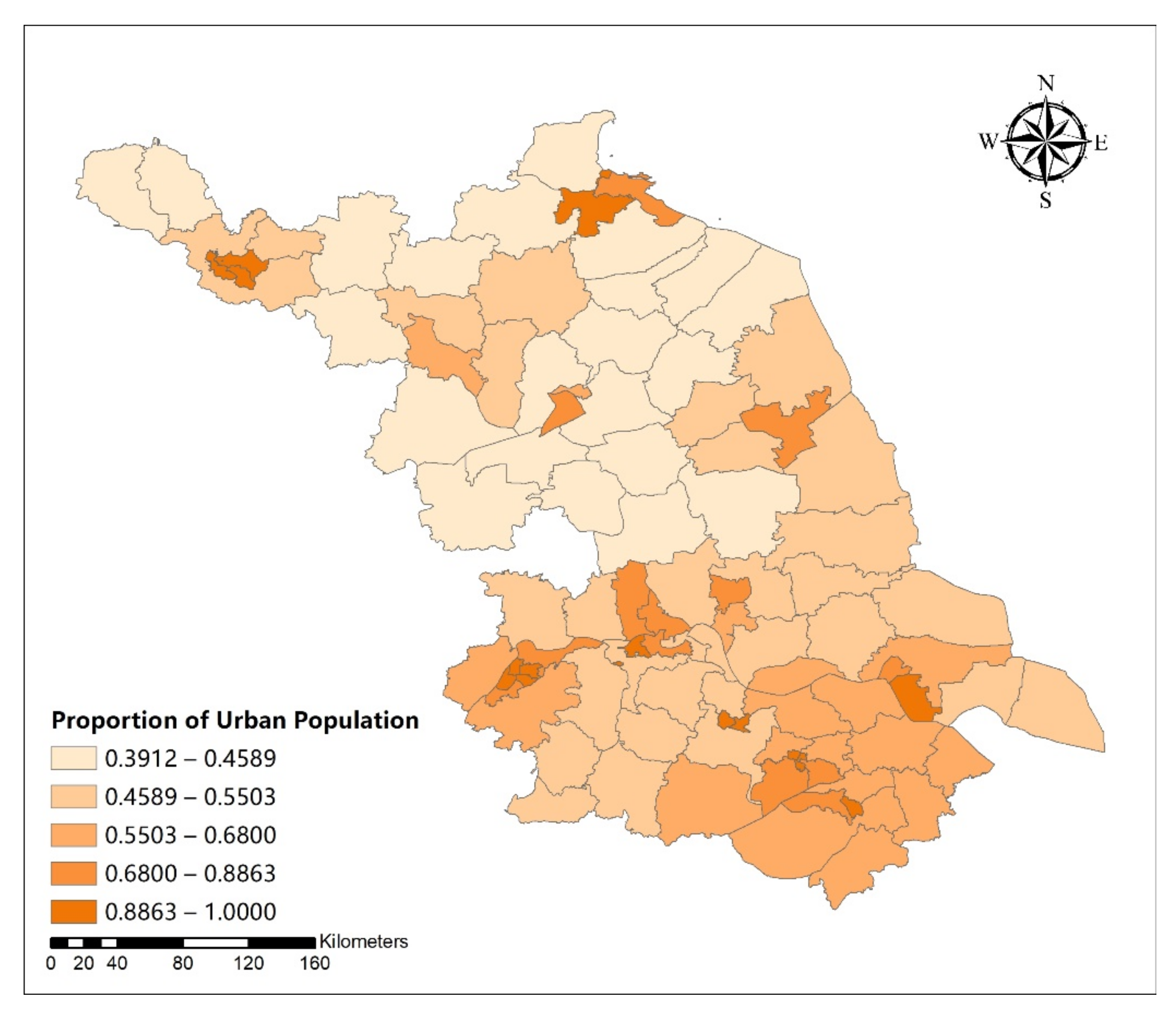
According to the spatial distribution of the estimated GWR coefficients and variable (Appendix A Figure A19, Figure A20, Figure A21 and Figure A22), the estimated coefficient of terrain undulation showed an increasing trend along the southeast direction, and the influence was greater in the areas with smaller terrain undulation in coastal areas. The estimated coefficient of population urbanization rate was the largest in the south of Jiangsu Province, and it was relatively small in the north of Jiangsu Province.
Table 10 shows that the σ ^ , R2, and adjusted-R2 were the same for OLS and GWR. The AICc was actually slightly larger for GWR compared to OLS. These results indicated that there was no benefit to using GWR rather than OLS. Note also that the R2 = 0.32 (2 DP) was low. This model explained 32% of the variability in urban distribution aggregation degree. By comparison, the first two models explained a large proportion of the variability in urban spatial expansion size (R2 = 0.82) and urban development intensity (R2 = 0.95).

4. Discussion

4.1. Statistical Methods for Studying Regional Urban Spatial Form

In this study, we applied methods from spatial statistics (Moran’s I, GWR) as well as conventional statistical methods. The use of spatial statistics allowed exploration and explanation of spatial patterns in the data which could not be obtained using conventional statistics. This is illustrated clearly in Figure 5 and Figure 6 (Section 3.1), which showed the clusters of low and high areas for urban spatial expansion size and urban spatial development intensity. The analysis for GWR did show patterns in the regression coefficients (Section 3.3); however, the actual variability in the coefficient was very small. This reinforced the results from the diagnostic statistics (Table 4, Table 7 and Table 10), which showed that GWR did not yield a better fit to the data than linear regression (OLS). This means that the patterns in urban spatial expansion size, urban development intensity, and urban distribution aggregation degree could be explained by the simpler OLS model. Hence, interpretation was not straightforward. Other studies (e.g., [28]) have found that GWR yielded improved results. The fact that OLS was sufficient in our study may reflect the availability of rich covariate information (Table 1) that could explain the spatial variability.

4.2. Unbalanced Development Characteristics of Regional Urban Spatial Form

Using the three dimensions of urban spatial expansion size, development intensity, and distribution aggregation degree, the characteristics of unbalanced regional urban spatial forms can be elucidated and understood. Due to data availability, we could only work with data from 2015. Hence, we cannot comment on the most recent situation. Studying the current and long-term unbalanced urban development is important and remains a topic for further research. The regional urban spatial form in Jiangsu Province will present different spatial patterns such as gradients, cluster, or random when we use different indicators. There is an apparent spatial correlation between urban spatial expansion size and development intensity (Figure 1 and Figure 2). In areas with larger urban spatial expansion size, the development intensity tends to be larger, resulting in the formation of urban agglomerations. For example, southern Jiangsu demonstrated this pattern vividly as both its urban spatial expansion size and development intensity were high. In contrast, in northern Jiangsu, where both the two indicators’ values are relatively low, there was a low density and scattered urban patches and the urban spatial expansion mainly occurred on the edges of the built-up areas. When the urban spatial distribution aggregation degree was used to measure the imbalance of regional urban spatial form, the results appeared to be random. Considering the spatial expansion size and density, we found that the development of urban clusters had reached a relatively mature stage in southern Jiangsu where the central cities being were linked with the surrounding towns. This was also illustrated in Figure 5 and Figure 6 when considering the high-high and low-low clustering of urban expansion size and urban development intensity.

4.3. Driving Mechanism of Unbalanced Regional Spatial Urban Form

We combined traditional statistical methods and spatial statistical methods and we explored the driving mechanism of unbalanced regional spatial urban form in detail. The economy was the fundamental driving variable of urban spatial expansion size [45,46] in Jiangsu Province. The counties or districts with larger industrial production and larger labor force are more likely to have more developed high-tech industries and bigger foreign trades, which will in turn enlarge the size of urban spatial expansion. In central Jiangsu, where there is a moderate size of urban spatial expansion, manufacturing and heavy industry are the region’s leading industries. Scientific and technological development stay in an early stage. Meanwhile, industrial development in northern Jiangsu is still resource-dependent and the industry and urban area are limited and scattered in space. Urbanization level and urbanization quality play major roles in driving the urban spatial development intensity in Jiangsu Province. With higher levels of urbanization, there will be higher transportation accessibility and closer connections of the population, which will in turn intensify the spatial development in the urban areas. The development intensity of urban space in southern Jiangsu was relatively high due to the good transportation network supporting tight population connections among the cities [47]. Central and northern Jiangsu have not yet formed mature regional transportation networks, resulting in relatively low development intensity. From the perspective that per capita GDP has a negative influence on urban spatial development intensity, perhaps there is also evidence that richer people prefer a less built-up living environment (e.g., house/villa rather than apartment). Moreover, according to Table 3, there was not a significant correlation between distance to Shanghai and urban development intensity. However, distance to Shanghai was a significant variable of urban development intensity in the OLS and GWR models. Shanghai is a coastal city, which is not only an important port but also an important economic gateway. It plays a unique leading role in the Yangtze River Delta and has a great impact on Jiangsu Province. Considering the variable of “distance to Shanghai”, we can not only consider the distance between districts and counties from the coastline to a certain extent but also reflect the influence of the developed surrounding metropolis on Jiangsu Province. Detailed results of models comparison can be seen in the Appendix A.2. Natural landform and urbanization level are major drivers of urban spatial distribution aggregation degree [48]. Complex topographies were associated with low urbanization levels and dispersed urban spatial layouts. These driving variables interacted and shared some correlation as well.

4.4. Optimization Strategies for a Balanced Development of Regional Urban Spatial Form

In southern Jiangsu, with its large urban spatial expansion size, high development intensity, and urban agglomeration, the economy and urbanization levels were relatively mature. In the future, measures that improve the spatial urban layout, i.e., promoting regional integration and urban–rural joint development, should be emphasized [49]. The urban integration of Nanjing City with Suzhou City, Wuxi City, and Changzhou City, which have distinctive and complementary advantages, should be encouraged to enhance the overall competitiveness of the region. Meanwhile, the transportation network and public infrastructure development should be planned and shared with a collaboration among the four key cities. This would form a mega-city area in the southern Jiangsu region. In central Jiangsu, where the urban spatial expansion size and distribution aggregation degree were relatively moderate and the urban spatial development intensity was relatively low, the future development strategy for Nanjing should focus on enhancing the intensity of urban development. The local government should make full use of the local coastline resources to promote the port and logistics industry development. At the same time, urban construction and upgrading can be promoted through industrial development. In northern Jiangsu where there was a scattered and small size of urban expansion and development intensity, measures to accelerate the improvement of the local economy should be prioritized. The emphasis should be put on some larger cities in the region, including Xuzhou City, Huaiyin City, Yancheng City, and Lianyungang City, which have the potential to become leading forces to accelerate the local urban spatial expansion as well as the public infrastructure and transportation network. This will, in turn, promote the growth of urban clusters with the central cities as cores [50].

5. Conclusions

Based on the general concern of unbalanced inter-regional development, this study aimed to reveal the characteristics and driving mechanism of unbalanced regional urban spatial form. In particular, we have used multiple indices. In terms of indicators of unbalanced development characteristics of urban spatial form, most previous studies still use a single indicator and lack multiple indicator analysis. As for driving mechanisms, comparison of the influencing variables of multiple unbalanced development characteristics is rare. Furthermore, in terms of research methods, the traditional statistical analysis does not allow the full exploration of spatial patterns in the data. In order to fill these research gaps, we used three indicators of urban spatial expansion size, development intensity, and distribution aggregation degree. In addition, spatial analysis tools and traditional statistical analysis tools were combined in this study. First, spatial autocorrelation analysis was used to analyze the characteristics of the unbalanced spatial form of towns in Jiangsu province. It was found that there is a positive spatial correlation between the urban spatial expansion size and development intensity. Specifically, the regions with large values of both were mainly in southern Jiangsu, while the regions with small values are mainly in northern Jiangsu. While the spatial distribution of cities and towns has no agglomeration phenomenon. Secondly, the Pearson Correlation Analysis, OLS, and GWR Analysis were applied to reveal the correlations and differences between various driving mechanisms, namely, economy, urbanization quality, urbanization level, and natural landform. It was found that urbanization level can lead to inter-regional imbalances of urban spatial development intensity and distribution aggregation degree at the same time. Finally, the optimization strategies were formulated to promote balanced development between regions in Jiangsu Province. Southern Jiangsu should focus on improving the urbanization quality and promote regional integration. Central Jiangsu should improve the urbanization level and develop along the axis relying on rapid transportation. Northern Jiangsu should expand the economic scale and build the urban agglomeration with central cities as the core.
Many variables affect the unbalanced development of inter-regional urban space and this study could not cover all possible variables. The significantly correlated variables could change over time. These two points should be considered in future studies.
Author Contributions

Conceptualization, G.X. and T.L.; methodology, X.C., N.A.S.H. and T.L.; software, X.C.; validation, X.C., G.Z. and N.A.S.H.; formal analysis, G.X., X.C. and T.L.; resources, X.C., G.Z. and B.C.; writing—original draft preparation, G.X. and X.C.; writing—review and editing, N.A.S.H. and T.L.; visualization, X.C.; funding acquisition, G.X. and T.L. All authors have read and agreed to the published version of the manuscript.

Funding

This research was funded by National Natural Science Foundation of China, grant number 51578129 and The APC was funded by SEU.

Institutional Review Board Statement

Not applicable.

Informed Consent Statement

Not applicable.

Data Availability Statement

Not applicable.

Conflicts of Interest

The authors declare no conflict of interest.

Appendix A

Appendix A.1. Spatial Distribution Map of Influencing Variables and Their Estimated Coefficients

Figure A1. Spatial distribution map of estimated coefficient of proportion of the population over 60 years old on urban spatial expansion size in Jiangsu Province.
Sustainability 13 03121 g0a1
Figure A2. Spatial distribution map of proportion of the population over 60 years old in Jiangsu Province.
Sustainability 13 03121 g0a2
Figure A3. Spatial distribution map of estimated coefficient of the total number of point of interest (POI) on urban spatial expansion size in Jiangsu Province.
Sustainability 13 03121 g0a3
Figure A4. Spatial distribution map of proportion of the total number of POI in Jiangsu Province.
Sustainability 13 03121 g0a4
Figure A5. Spatial distribution map of estimated coefficient of the output of secondary industry on urban spatial expansion size in Jiangsu Province.
Sustainability 13 03121 g0a5
Figure A6. Spatial distribution map of proportion of the output of secondary industry in Jiangsu Province.
Sustainability 13 03121 g0a6
Figure A7. Spatial distribution map of estimated coefficient of total export–import volume on urban spatial expansion size in Jiangsu Province.
Sustainability 13 03121 g0a7
Figure A8. Spatial distribution map of total export–import volume in Jiangsu Province.
Sustainability 13 03121 g0a8
Figure A9. Spatial distribution map of estimated coefficient of income of national and provincial.
Sustainability 13 03121 g0a9
Figure A10. Spatial distribution map of income of national and provincial development zones in Jiangsu Province.
Sustainability 13 03121 g0a10
Figure A11. Spatial distribution map of estimated coefficient of road density on urban development intensive in Jiangsu Province.
Sustainability 13 03121 g0a11
Figure A12. Spatial distribution map of road density in Jiangsu Province.
Sustainability 13 03121 g0a12
Figure A13. Spatial distribution map of estimated coefficient of urban population density on urban development intensive in Jiangsu Province.
Sustainability 13 03121 g0a13
Figure A14. Spatial distribution map of urban population density in Jiangsu Province.
Sustainability 13 03121 g0a14
Figure A15. Spatial distribution map of estimated coefficient of distance to Shanghai of districts and counties on urban development intensive in Jiangsu Province.
Sustainability 13 03121 g0a15
Figure A16. Spatial distribution map of distance to Shanghai of districts and counties in Jiangsu Province.
Sustainability 13 03121 g0a16
Figure A17. Spatial distribution map of estimated coefficient of per capita GDP on urban development intensive in Jiangsu Province.
Sustainability 13 03121 g0a17
Figure A18. Spatial distribution map of per capita GDP in Jiangsu Province.
Sustainability 13 03121 g0a18
Figure A19. Spatial distribution map of estimated coefficient of terrain undulation on urban distribution aggregation degree in Jiangsu Province.
Sustainability 13 03121 g0a19
Figure A20. Spatial distribution map of terrain undulation in Jiangsu Province.
Sustainability 13 03121 g0a20
Figure A21. Spatial distribution map of estimated coefficient of proportion of urban population on urban distribution aggregation degree in Jiangsu Province.
Sustainability 13 03121 g0a21
Figure A22. Spatial distribution map of the proportion of urban population in Jiangsu Province.
Sustainability 13 03121 g0a22
Figure A23. Spatial distribution map of the mean digital elevation model (DEM) in Jiangsu Province.
Sustainability 13 03121 g0a23

Appendix A.2. Models Comparison Results of Influencing Variables of Urban Spatial Development Intensity

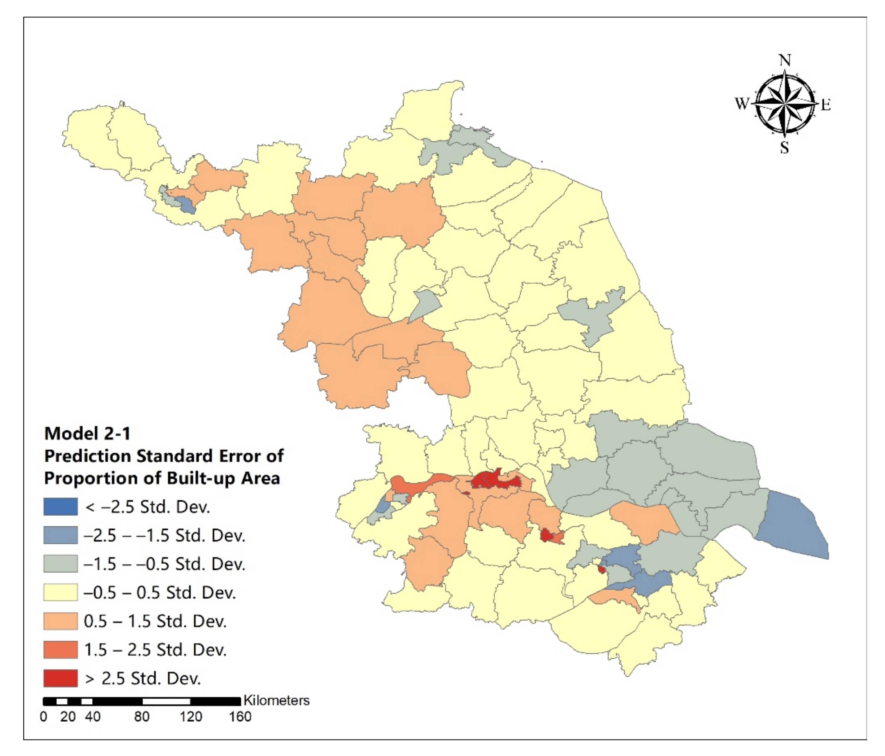
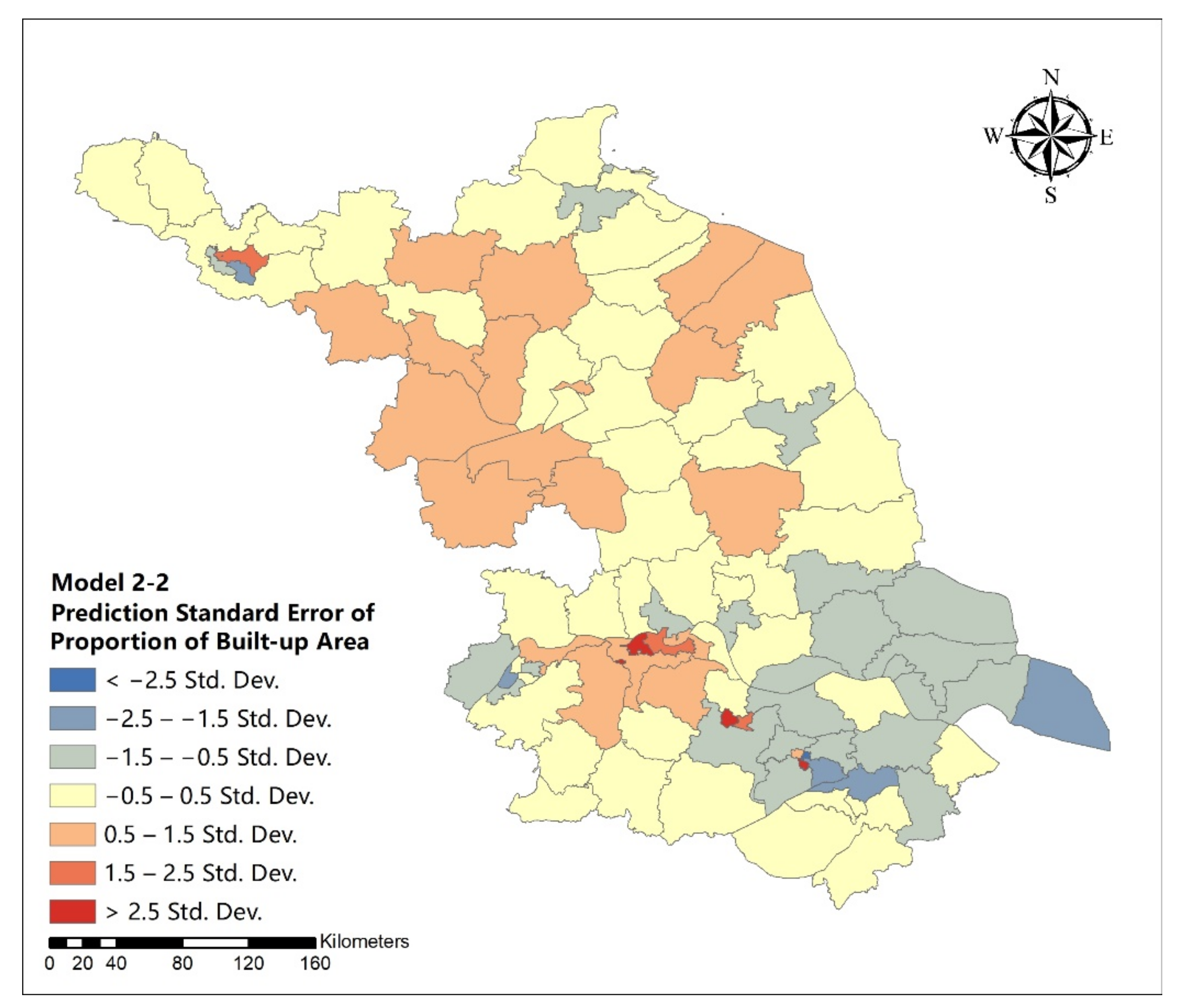
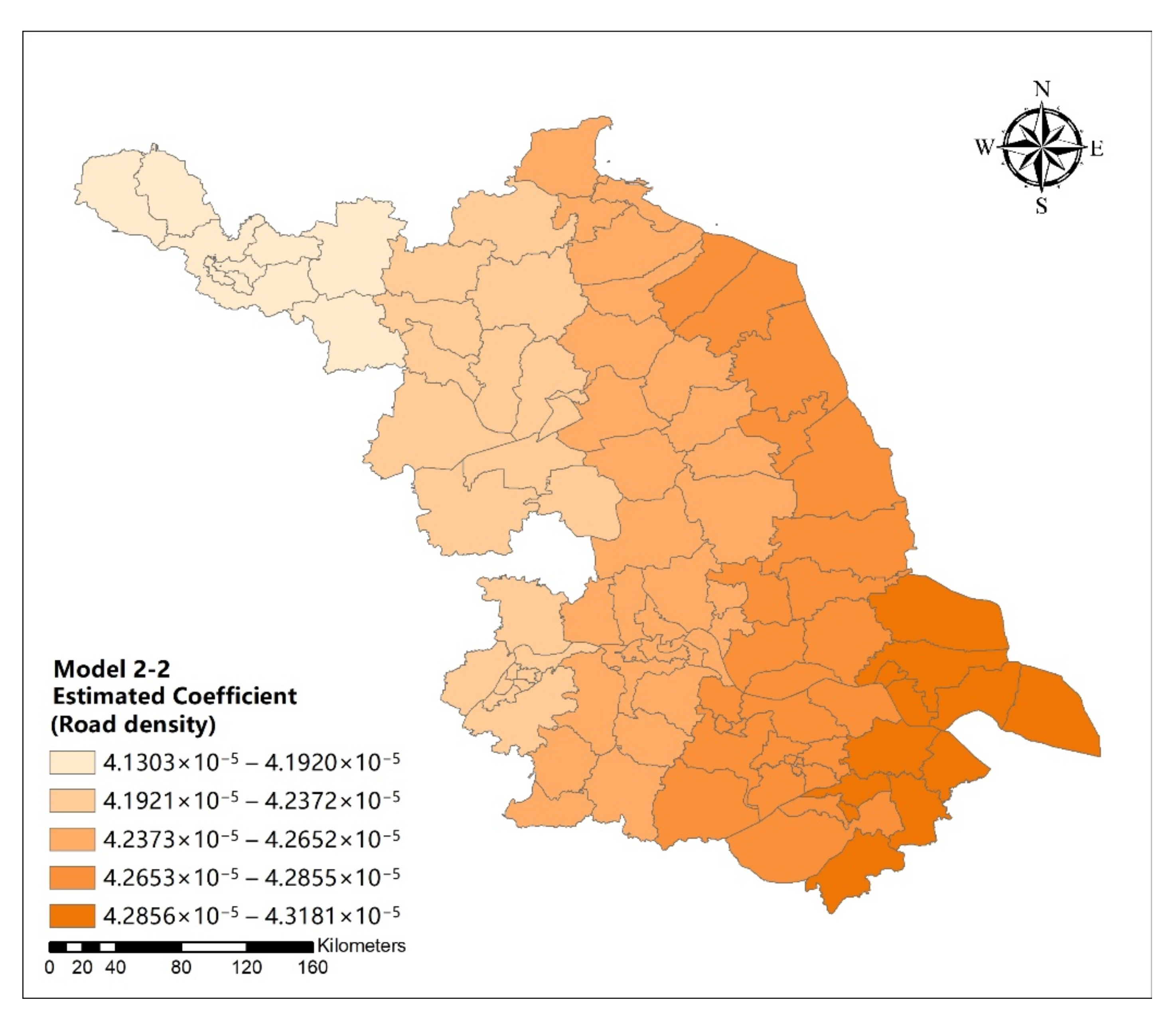
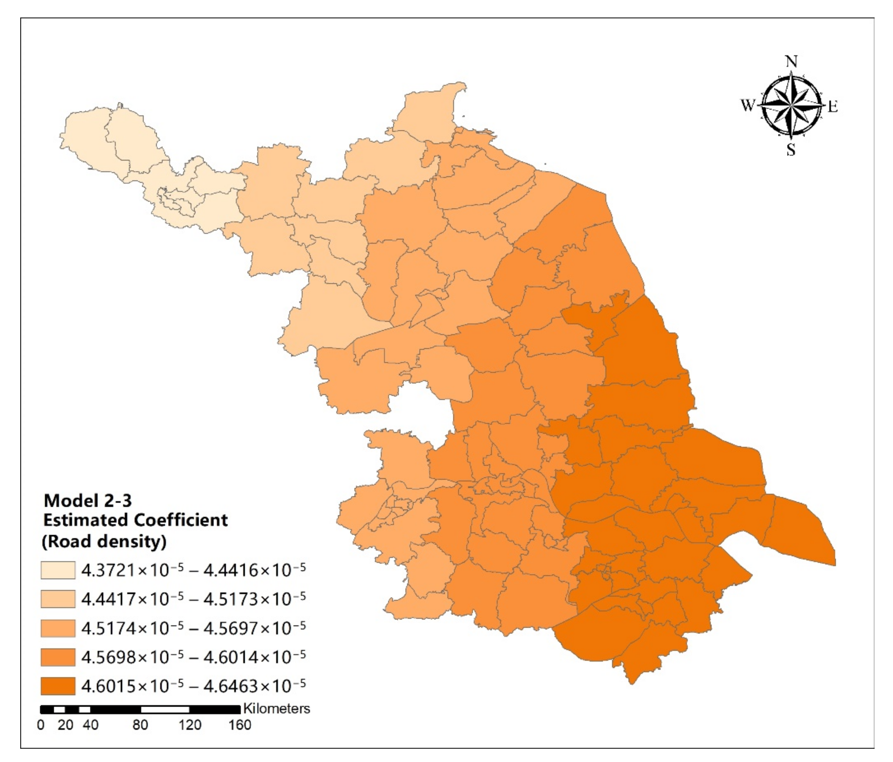
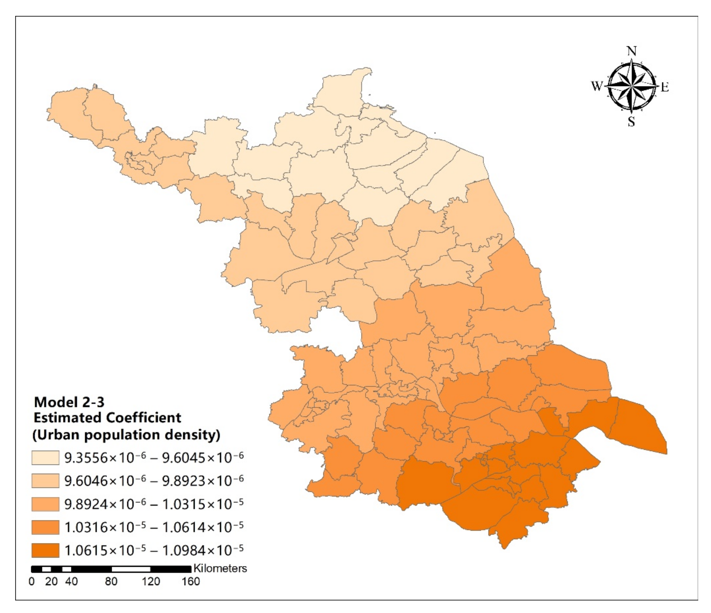
Compared with the model in Section 3.3.2, OLS and GWR model 2-1 remove distance to Shanghai, OLS and GWR model 2-2 remove distance to Shanghai and per capita GDP, and OLS and GWR model 2-3 remove per capita GDP. Among these models, OLS model 2-2 was clearly the worst performing model since AIC is the largest and R2 and adjusted R2 are the lowest. According to AIC, OLS and GWR model in 3.3.2 was the best performing, although R2 and adjusted R2 were similar to model 2-1. Therefore, it is better to choose the model in 3.3.2 for OLS.
For GWR, AIC of model 2-2 was similar to the model presented in Section 3.3.2, but model 2-2 is more simple because it only has two covariates. The spatially varying coefficients in GWR allowed us to account for variability in urban development intensity without adding more covariates. Therefore, these results show that adopting model 2-2 could be justified, but there are also other reasonable choices, in particular the model adopted in Section 3.3.2. The sign of the estimated coefficient of distance to Shanghai is positive in GWR for model 2-3. This model does not include the covariate of per capita GDP, which suggests that the sign change in the model presented in Section 3.3.2 may be caused by the co-effect of per capita GDP. Note also that the bivariate correlation between urban development intensity and distance to Shanghai (Table 3) was not significantly different from zero.
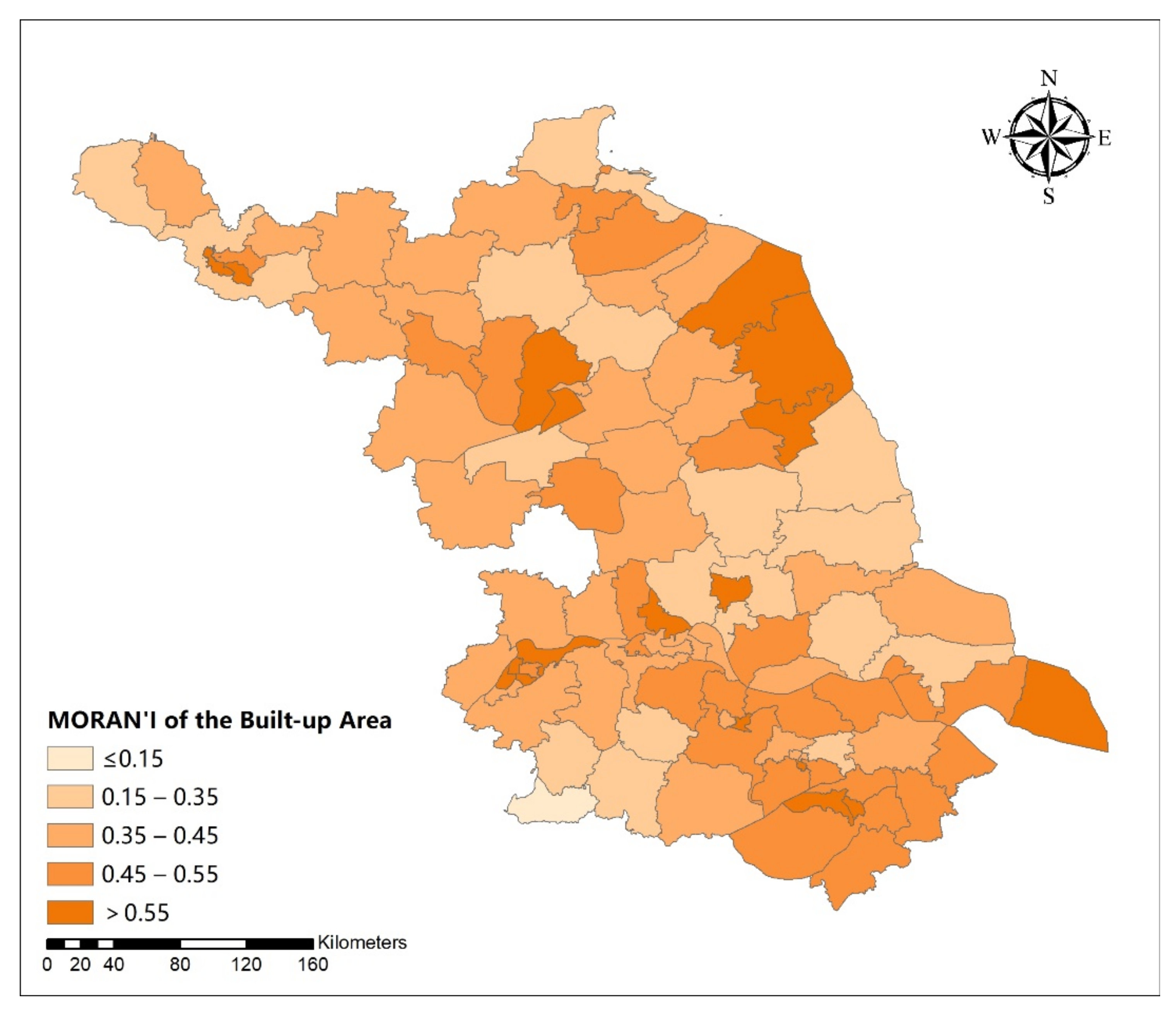
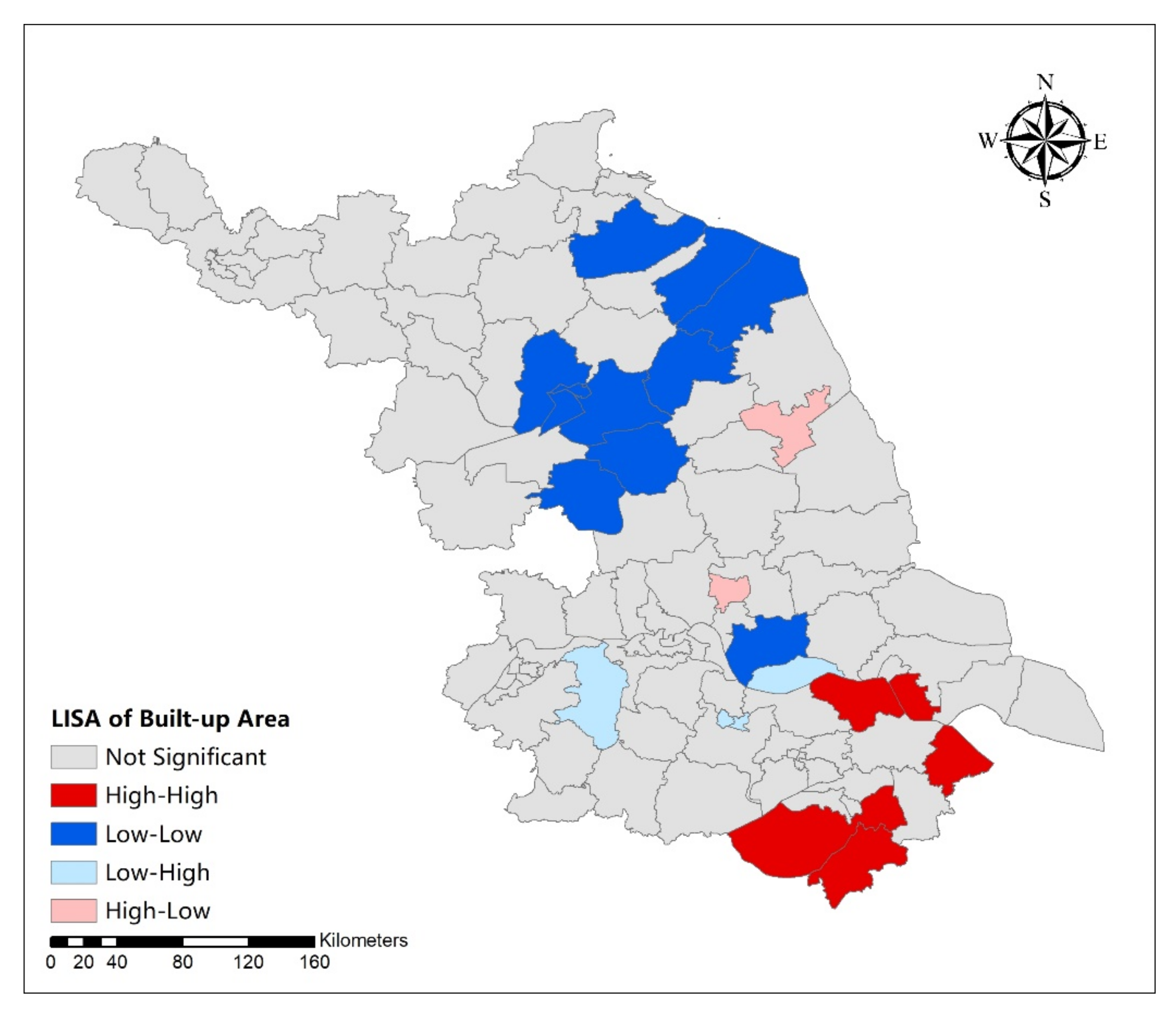
Table A1. Summary of OLS and GWR model 2-1 of influencing variables of urban development intensive in Jiangsu Province.
IDStatisticsOLS Model ParametersGWR Model Parameters
1σ0.03940.0394
2AICc−355.3750−352.7313
3R20.94460.9446
4R2 Adjusted0.94280.9428
Table A2. Estimated coefficients of OLS regression model 2-1 for influencing variables of urban development intensive in Jiangsu Province.
Influence VariablesCoefficientsStandard ErrorStandardized Coefficientstp-Value
Constant−0.03889.5918 × 10−3 −4.04900.0001
Road density4.7599 × 10−51.1112 × 10−70.8131−3.64870.0004
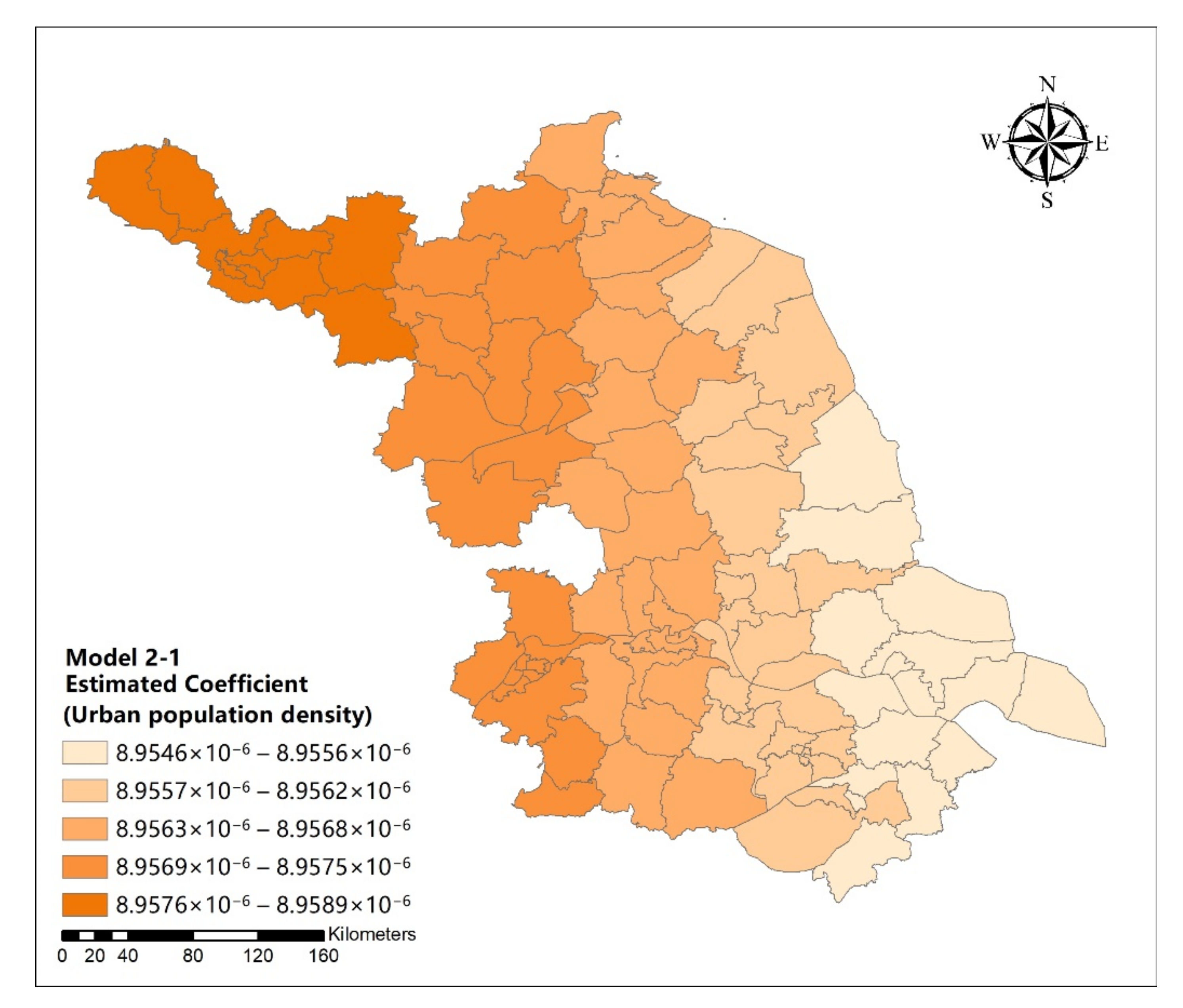
Urban population density8.9568 × 10−61.9739 × 10−60.21664.53760.0000
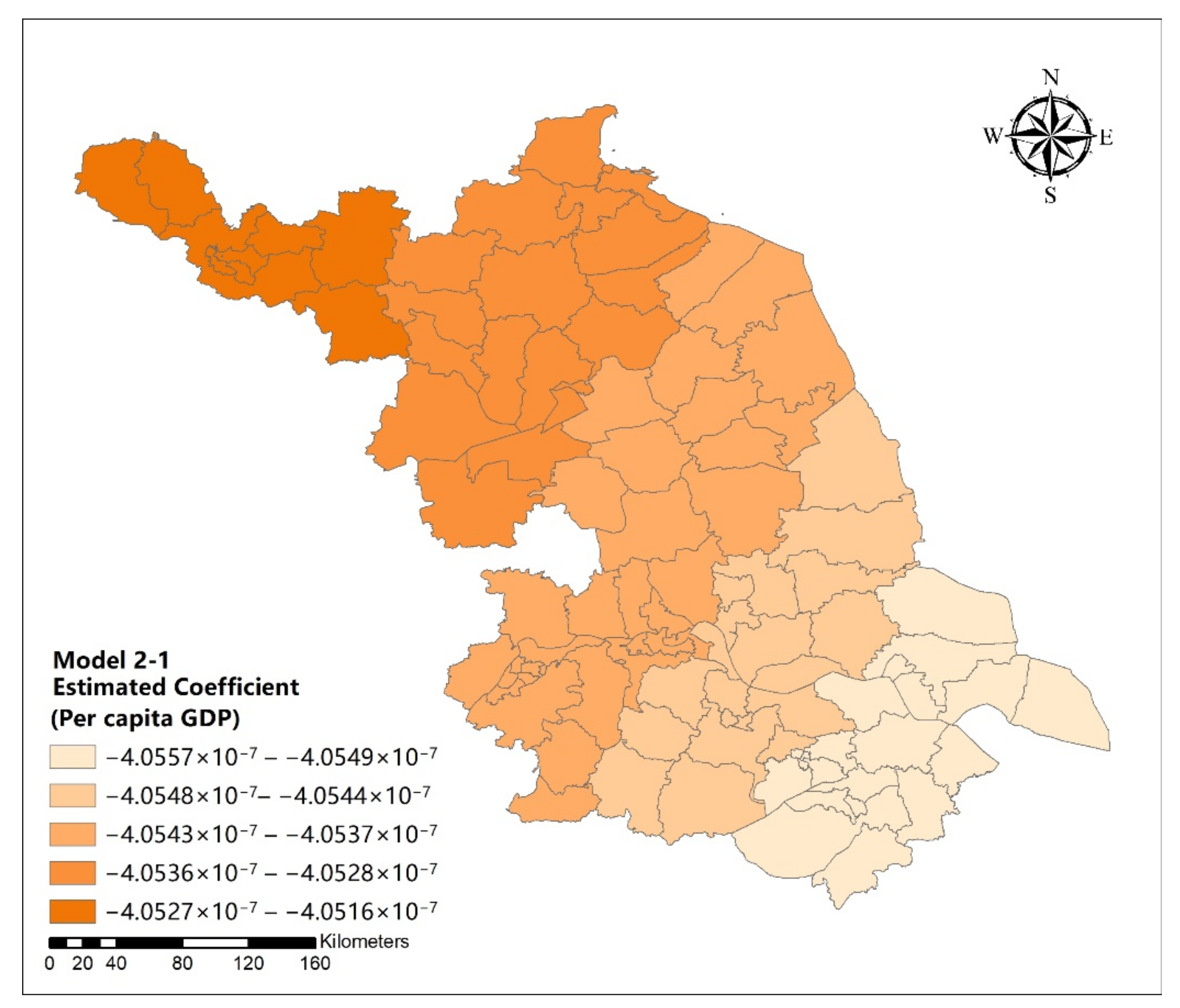
Per capita GDP−4.0544 × 10−72.9950 × 10−6−0.102915.89270.0000
Table A3. Estimated coefficients of GWR regression model 2-1 for influencing variables of urban development intensive in Jiangsu Province.
StatisticsConstantRoad DensityUrban Population DensityPer Capita GDP
Minimum−3.8846 × 10−24.7591 × 10−58.9546 × 10⁻⁶−4.0557 × 10⁻⁷
Lower quartile−3.8840 × 10−24.7597 × 10−58.9558 × 10⁻⁶−4.0548 × 10⁻⁷
Median−3.8837 × 10−24.7599 × 10−58.9564 × 10⁻⁶−4.0542 × 10⁻⁷
Upper quartile−3.8834 × 10−24.7601 × 10−58.9570 × 10⁻⁶−4.0535 × 10⁻⁷
Maximum−3.8823 × 10−24.7604 × 10−58.9589 × 10⁻⁶−4.0516 × 10⁻⁷
Table A4. Summary of OLS and GWR model 2-2 of influencing variables of urban development intensive in Jiangsu Province.
IDStatisticsOLS Model ParametersGWR Model Parameters
1σ0.04190.0386
2AICc−344.3910−356.1783
3R20.93680.9479
4R2 Adjusted0.93550.9451
Table A5. Estimated coefficients of OLS regression model 2-2 for influencing variables of urban development intensive in Jiangsu Province.
Influence VariablesCoefficientsStandard ErrorStandardized Coefficientstp-Value
Constant−6.6062 × 10−26.4024 × 10−3 −10.31830.0000
Road density4.2090 × 10−52.7475 × 10−60.719015.31950.0000
Urban population density1.1679 × 10−51.9411 × 10−60.28246.01700.0000
Table A6. Estimated coefficients of GWR regression model 2-2 for influencing variables of urban development intensive in Jiangsu Province.
StatisticsConstantRoad DensityUrban Population Density
Minimum−0.08194.1303 × 10−51.0126 × 10⁻⁵
Lower quartile−0.07364.2338 × 10−51.0790 × 10⁻⁵
Median−0.06734.2584 × 10−51.1688 × 10⁻⁵
Upper quartile−0.05944.2778 × 10−51.2219 × 10⁻⁵
Maximum−0.05074.3181 × 10−51.2914 × 10⁻⁵
Table A7. Summary of OLS and GWR model 2-3 of influencing variables of urban development intensive in Jiangsu Province.
IDStatisticsOLS Model ParametersGWR Model Parameters
1σ0.03960.0402
2AICc−354.3870−349.3812
3R20.94400.9435
4R2 Adjusted0.94230.9406
Table A8. Estimated coefficients of OLS regression model 2-3 for influencing variables of urban development intensive in Jiangsu Province.
Influence VariablesCoefficientsStandard ErrorStandardized Coefficientstp-Value
Constant−1.0106 × 10−11.1696 × 10−2 −8.64090.0000
Road density4.5714 × 10−52.7983 × 10−60.242616.33600.0000
Urban population density1.0035 × 10−51.8958 × 10−60.78095.29350.0000
Distance to Shanghai9.5004 × 10−52.7158 × 10−50.09223.49830.0007
Table A9. Estimated coefficients of GWR regression model 2-3 for influencing variables of urban development intensive in Jiangsu Province.
StatisticsConstantRoad DensityUrban Population DensityDistance to Shanghai
Minimum−0.12104.3721 × 10−59.3556 × 10−64.5310 × 10−5
Lower quartile−0.11114.5522 × 10−59.7236 × 10−68.9686 × 10−5
Median−0.10484.5832 × 10−51.0202 × 10−51.1073 × 10−4
Upper quartile−0.09604.6080 × 10−51.0530 × 10−51.2704 × 10−4
Maximum−0.07504.6463 × 10−51.0984 × 10−51.5359 × 10−4
Figure A24. Standard error map of GWR model for influencing variables of urban development intensive in Jiangsu Province (model 2-1).
Sustainability 13 03121 g0a24
Figure A25. Spatial distribution map of estimated coefficient of road density on urban development intensive in Jiangsu Province (model 2-1).
Sustainability 13 03121 g0a25
Figure A26. Spatial distribution map of estimated coefficient of urban population density on urban development intensive in Jiangsu Province (model 2-1).
Sustainability 13 03121 g0a26
Figure A27. Spatial distribution map of estimated coefficient of per capita GDP on urban development intensive in Jiangsu Province (model 2-1).
Sustainability 13 03121 g0a27
Figure A28. Standard error map of GWR model for influencing variables of urban development intensive in Jiangsu Province (model 2-2).
Sustainability 13 03121 g0a28
Figure A29. Spatial distribution map of estimated coefficient of road density on urban development intensive in Jiangsu Province (model 2-2).
Sustainability 13 03121 g0a29
Figure A30. Spatial distribution map of estimated coefficient of urban population density on urban development intensive in Jiangsu Province (model 2-2).
Sustainability 13 03121 g0a30
Figure A31. Standard error map of GWR model for influencing variables of urban development intensive in Jiangsu Province (model 2-3).
Sustainability 13 03121 g0a31
Figure A32. Spatial distribution map of estimated coefficient of road density on urban development intensive in Jiangsu Province (model 2-3).
Sustainability 13 03121 g0a32
Figure A33. Spatial distribution map of estimated coefficient of urban population density on urban development intensive in Jiangsu Province (model 2-3).
Sustainability 13 03121 g0a33
Figure A34. Spatial distribution map of estimated coefficient of distance to Shanghai of districts and counties on urban development intensive in Jiangsu Province (model 2-3).
Sustainability 13 03121 g0a34

References

  1. Sukkoo, K. Spatial Inequality and Economic Development; The World Bank: Washington, DC, USA, 2008; pp. 12–24. [Google Scholar]
  2. Wei, Y.D.; Ewing, R. Urban expansion, sprawl and inequality. Landsc. Urban Plan. 2018, 177, 259–265. [Google Scholar] [CrossRef]
  3. Desponds, D.; Auclair, E. The new towns around Paris 40 years later: New dynamic centralities or suburbs facing risk of marginalisation? Urban Stud. 2017, 54, 862–877. [Google Scholar] [CrossRef]
  4. Green, M.A. Mapping Inequality in London: A Different Approach. Cartogr. J. 2012, 49, 247–255. [Google Scholar] [CrossRef] [Green Version]
  5. Farrell, L.J.; Kenyon, P.R.; Morris, S.T.; Tozer, P.R. The Impact of Hogget and Mature Flock Reproductive Success on Sheep Farm Productivity. Agriculture 2020, 10, 566. [Google Scholar] [CrossRef]
  6. Zarifa, D.; Seward, B.; Milian, R.P. Location, location, location: Examining the rural-urban skills gap in Canada. J. Rural Stud. 2019, 72, 252–263. [Google Scholar] [CrossRef]
  7. Palit, A. Examining the Regional Imbalance in China: Comparison with India. In Regional Development and Public Policy Challenges in India; Bhattacharya, R., Ed.; Springer: New Delhi, India, 2015; pp. 291–307. [Google Scholar]
  8. Dutta, I.; Das, A. Application of geo-spatial indices for detection of growth dynamics and forms of expansion in English Bazar Urban Agglomeration, West Bengal. J. Urban Manag. 2019, 8, 288–302. [Google Scholar] [CrossRef]
  9. Masud, J.; Haron, S.A. Income differences among elderly in Malaysia: A regional comparison. Int. J. Consum. Stud. 2008, 32, 335–340. [Google Scholar] [CrossRef]
  10. Roman, M.; Roman, M.; Prus, P.; Szczepanek, M. Tourism Competitiveness of Rural Areas: Evidence from a Region in Poland. Agriculture 2020, 10, 569. [Google Scholar] [CrossRef]
  11. Ervin, P.A.; Bubak, V. Closing the rural-urban gap in child malnutrition: Evidence from Paraguay, 1997–2012. Econ. Hum. Biol. 2019, 32, 1–10. [Google Scholar] [CrossRef] [PubMed]
  12. Xu, D.; Hou, G.L. The Spatiotemporal Coupling Characteristics of Regional Urbanization and Its Influencing Factors: Taking the Yangtze River Delta as an Example. Sustainability 2019, 11, 822. [Google Scholar] [CrossRef] [Green Version]
  13. Wan, J.; Zhang, L.W.; Yan, J.P.; Wang, X.M.; Wang, T. Spatial—Temporal Characteristics and Influencing Factors of Coupled Coordination between Urbanization and Eco-Environment: A Case Study of 13 Urban Agglomerations in China. Sustainability 2020, 12, 8821. [Google Scholar] [CrossRef]
  14. Wei, Y.D.; Li, H.; Yue, W.Z. Urban land expansion and regional inequality in transitional China. Landsc. Urban Plan. 2017, 163, 17–31. [Google Scholar] [CrossRef]
  15. Fang, C.L.; Liu, X.L. Temporal and spatial differences and imbalance of China’s urbanization development during 1950–2006. J. Geogr. Sci. 2009, 19, 719–732. [Google Scholar] [CrossRef]
  16. Bonilla-Bedoya, S.; Mora, A.; Vaca, A.; Estrella, A.; Herrera, M.Á. Modelling the relationship between urban expansion processes and urban forest characteristics: An application to the Metropolitan District of Quito. Comput. Environ. Urban Syst. 2020, 79, 101420. [Google Scholar] [CrossRef]
  17. Wang, S.J.; Fang, C.L.; Wang, Y.; Huang, Y.B.; Ma, H.T. Quantifying the relationship between urban development intensity and carbon dioxide emissions using a panel data analysis. Ecol. Indic. 2015, 49, 121–131. [Google Scholar] [CrossRef]
  18. Wang, D.C.; Chen, W.G.; Wei, W.; Bird, B.W.; Zhang, L.H.; Sang, M.Q.; Wang, Q.Q. Research on the Relationship between Urban Development Intensity and Eco-Environmental Stresses in Bohai Rim Coastal Area, China. Sustainability 2016, 8, 15. [Google Scholar] [CrossRef] [Green Version]
  19. Hu, C.; Liu, W.; Jia, Y.; Jin, Y. Characterization of Territorial Spatial Agglomeration Based on POI Data: A Case Study of Ningbo City, China. Sustainability 2019, 11, 5083. [Google Scholar] [CrossRef] [Green Version]
  20. Ebeke, C.H.; Ntsama Etoundi, S.M. The Effects of Natural Resources on Urbanization, Concentration, and Living Standards in Africa. World Dev. 2017, 96, 408–417. [Google Scholar] [CrossRef]
  21. Shao, Z.; Ding, L.; Li, D.; Altan, O.; Huq, M.E.; Li, C. Exploring the Relationship between Urbanization and Ecological Environment Using Remote Sensing Images and Statistical Data: A Case Study in the Yangtze River Delta, China. Sustainability 2020, 12, 5620. [Google Scholar] [CrossRef]
  22. Li, S.J.; Zhou, C.S.; Wang, S.J.; Gao, S.; Liu, Z.T. Spatial Heterogeneity in the Determinants of Urban Form: An Analysis of Chinese Cities with a GWR Approach. Sustainability 2019, 11, 479. [Google Scholar] [CrossRef] [Green Version]
  23. Jones, C.; Henderson, D. Broadband and uneven spatial development: The case of Cardiff City-Region. Local Econ. J. Local Econ. Policy Unit 2019, 34, 228–247. [Google Scholar] [CrossRef]
  24. Farmer, S. Uneven Public Transportation Development in Neoliberalizing Chicago, USA. Environ. Plan. A Econ. Space 2011, 43, 1154–1172. [Google Scholar] [CrossRef]
  25. Ye, C.; Liu, Z.J.; Cai, W.B.; Chen, R.S.; Liu, L.L.; Cai, Y.L. Spatial Production and Governance of Urban Agglomeration in China 2000–2015: Yangtze River Delta as a Case. Sustainability 2019, 11, 1343. [Google Scholar] [CrossRef] [Green Version]
  26. Salvati, L.; Venanzoni, G.; Carlucci, M. Towards (spatially) unbalanced development? A joint assessment of regional disparities in socioeconomic and territorial variables in Italy. Land Use Policy 2016, 51, 229–235. [Google Scholar] [CrossRef]
  27. Sangkasem, K.; Puttanapong, N. Analysis of Spatial Inequality using DMSP/OLS Nighttime Light Satellite Imageries: A Case Study of Thailand. Reg. Sci. Policy Pract. 2020. [Google Scholar] [CrossRef]
  28. Ansong, D.; Ansong, E.K.; Ampomah, A.O.; Adjabeng, B.K. Factors contributing to spatial inequality in academic achievement in Ghana: Analysis of district-level factors using geographically weighted regression. Appl. Geogr. 2015, 62, 136–146. [Google Scholar] [CrossRef]
  29. Oduro, C.Y.; Peprah, C.; Adamtey, R. Analysis of the Determinants of Spatial Inequality in Ghana Using Two-Stage Least-Square Regression. Dev. Ctry. Stud. 2014, 4, 28–44. [Google Scholar]
  30. Falzetti, P.; Sacco, C. Analysis of school-level factors contributing to spatial inequality in academic achievement in Italy. INVALSI 2020, 44, 1–16. [Google Scholar]
  31. Naimi, B.; Hamm, N.A.S.; Groen, T.A.; Skidmore, A.K.; Toxopeus, A.G.; Alibakhshi, S. ELSA: Entropy-based local indicator of spatial association. Spat. Stat. 2019, 29, 66–88. [Google Scholar] [CrossRef]
  32. Odongo, V.O.; Hamm, N.A.S.; Milton, E.J. Spatio-Temporal Assessment of Tuz Gölü, Turkey as a Potential Radiometric Vicarious Calibration Site. Remote Sens. 2014, 6, 2494–2513. [Google Scholar] [CrossRef] [Green Version]
  33. Hamm, N.A.S.; Finley, A.; Schaap, M.; Stein, A. A spatially varying coefficient model for mapping PM10 air quality at the European scale. Atmos. Environ. 2015, 102, 393–405. [Google Scholar] [CrossRef]
  34. Finley, A.O. Comparing spatially-varying coefficients models for analysis of ecological data with non-stationary and anisotropic residual dependence. Methods Ecol. Evol. 2010, 2, 143–154. [Google Scholar] [CrossRef]
  35. Brunsdon, C.; Fotheringham, A.S.; Charlton, M.E. Charlton Geographically Weighted Regression: A Method for Exploring Spatial Nonstationarity. Geogr. Anal. 1996, 28, 281–298. [Google Scholar] [CrossRef]
  36. Ju, H.; Zhang, Z.; Zuo, L.; Wang, J.; Zhang, S.; Wang, X.; Zhao, X. Driving forces and their interactions of built-up land expansion based on the geographical detector—A case study of Beijing, China. Int. J. Geogr. Inf. Sci. 2016, 30, 2188–2207. [Google Scholar] [CrossRef]
  37. Neter, J.; Kutner, M.H.; Nachtsheim, C.J.; Wasserman, W. Applied Linear Statistical Models, 4th ed.; WCB McGraw-Hill: New York, NY, USA, 1996. [Google Scholar]
  38. Karl, P. Notes on the history of correlation. Biometrika 1920, 13, 25–45. [Google Scholar]
  39. Schabenberger, O.; Gotway, C.A. Statistical Methods for Spatial Data Analysis; Chapman and Hall/CRC: Boca Raton, FL, USA, 2005. [Google Scholar]
  40. Moran, P.A. Notes on continuous stochastic phenomena. Biometrika 1950, 37, 17–23. [Google Scholar] [CrossRef]
  41. Anselin, L. Local Indicator of Spatial Association—LISA. Geogr. Anal. 1995, 27, 93–115. [Google Scholar] [CrossRef]
  42. Anselin, L. GeoDa: An Introduction to Spatial Data Analysis. Geogr. Anal. 2006, 38, 87. [Google Scholar] [CrossRef]
  43. Chatterjee, S.; Hadi, A.S. Regression Analysis by Example, 5th ed.; John Wiley & Sons: Hoboken, NJ, USA, 2012. [Google Scholar]
  44. Fotheringham, A.; Brunsdon, C.; Charlton, M. Geographically Weighted Regression: The Analysis of Spatially Varying Relationships; John Wiley & Sons: Hoboken, NJ, USA, 2002; Volume 13. [Google Scholar]
  45. Scott, F.A.J. Industrial Agglomeration and Development: A Survey of Spatial Economic Issues in East Asia and a Statistical Analysis of Chinese Regions. Econ. Geogr. 2003, 79, 295–319. [Google Scholar]
  46. Zhang, Y.S.; Lu, X.; Liu, B.Y.; Wu, D.T. Impacts of Urbanization and Associated Factors on Ecosystem Services in the Beijing-Tianjin-Hebei Urban Agglomeration, China: Implications for Land Use Policy. Sustainability 2018, 10, 4334. [Google Scholar] [CrossRef] [Green Version]
  47. Gerritse, M.; Arribas-Bel, D. Concrete agglomeration benefits: Do roads improve urban connections or just attract more people? Reg. Stud. 2018, 52, 1134–1149. [Google Scholar] [CrossRef] [Green Version]
  48. Luo, J.; Shi, P.J.; Zhang, X.B. Relationship between Topographic Factors and Population Distribution in Lanzhou-Xining Urban Agglomeration. Econ. Geogr. 2020, 40, 106–115. [Google Scholar]
  49. He, J.; Li, C.; Yu, Y.; Liu, Y.; Huang, J. Measuring urban spatial interaction in Wuhan Urban Agglomeration, Central China: A spatially explicit approach. Sustain. Cities Soc. 2017, 32, 569–583. [Google Scholar] [CrossRef]
  50. Wang, J.; Fang, C. New-type driving forces of urban agglomerations development in China. Geogr. Res. 2011, 30, 335–347. [Google Scholar]
Figure 1. Location of Jiangsu Province and its prefecture-level city.
Sustainability 13 03121 g001
Figure 2. Urban spatial expansion size of districts and counties in Jiangsu Province.
Sustainability 13 03121 g002
Figure 3. Urban development intensity in districts and counties of Jiangsu Province.
Sustainability 13 03121 g003
Figure 4. Urban aggregation degree of districts and counties in Jiangsu Province.
Sustainability 13 03121 g004
Figure 5. Local indicators of spatial association (LISA) (Local Moran’s I) cluster map of urban expansion size in Jiangsu Province.
Sustainability 13 03121 g005
Figure 6. Local indicators of spatial association (LISA) (Local Moran’s I) cluster map of urban development intensity in Jiangsu Province.
Sustainability 13 03121 g006
Table 1. Potential variables of urban spatial form.
Types of VariablesInfluencing Variables
Physical geographyArea of districts and counties, average elevation, terrain undulation, proportion of urban blue and green space, distance to Shanghai
EconomyGDP, per capita GDP, output value of primary industry, output of secondary industry, output value of tertiary industry, proportion of primary industrial output-value, proportion of secondary industrial output-value, proportion of tertiary industrial output-value per capita disposable income, total retail sales of consumer goods, total sales of wholesale and retail, total export–import volume, number of national and provincial development zones, income of national and provincial development zones
SocietyTotal population, urban population, rural population, proportion of population aged 15–59, proportion of population over 60 years old, proportion of urban population, density of urban population, number of colleges and universities, fixed asset investment, road density, and total number of POI
Table 2. Global spatial autocorrelation of urban form indicators in Jiangsu Province.
Urban Spatial Form IndicatorsMoran’ IZ Valuep-Value
Spatial expansion size0.2123.58680.003
Development intensity0.3946.70490.001
Distribution aggregation degree0.0761.42220.081
Table 3. Correlation coefficients of 30 potential variables of urban spatial form in Jiangsu Province.
Potential
Variables
The Urban Spatial Expansion SizeThe Urban Development
Intensity
The Urban Distribution
Aggregation Degree
Pearson
Correlation
Significance Test (Two-Sided)Pearson
Correlation
Significance Test (Two-Sided)Pearson
Correlation
Significance Test (Two-Sided)
Area of districts and counties0.0280.784−0.633 **0.000−0.394 **0.000
Average elevation0.0030.9760.0690.500−0.1270.212
Terrain undulation0.239 *0.017−0.1260.215−0.213 *0.035
Proportion of urban blue and green space0.208 *0.039−0.1250.218−0.0370.713
Distance to Shanghai−0.299 **0.003−0.1820.071−0.1130.265
GDP0.794 **0.0000.0420.6810.0300.765
Per capita GDP0.455 **0.0000.233 *0.0210.0360.720
Output value of primary industry−0.0220.829−0.609 **0.000−0.417 **0.000
Output of the secondary industry0.780 **0.000−0.1730.086−0.0640.531
Output value of tertiary industry0.683 **0.0000.359 **0.0000.1830.070
Proportion of primary industrial output-value−0.334 **0.001−0.563 **0.000−0.341 **0.001
Proportion of secondary industrial output-value0.281 **0.005−0.654 **0.000−0.336 **0.001
Proportion of tertiary industrial output-value−0.1140.2610.783 **0.0000.408 **0.000
Per capita disposable income0.402 **0.0000.668 **0.0000.369 **0.000
Total retail sales of consumer goods0.514 **0.0000.559 **0.0000.340 **0.001
Total sales of wholesale and retail0.537 **0.0000.393 **0.0000.287 **0.004
Total export-import volume0.615 **0.0000.0580.5720.1280.206
Number of national and provincial development zones0.358 **0.000−0.347 **0.000−0.0300.766
Income of national and provincial development zones0.654 **0.000−0.1980.050−0.0150.886
Total population0.581 **0.000−0.1040.304−0.0170.869
Urban population0.573 **0.0000.376 **0.0000.302 **0.002
Rural population0.258 **0.010−0.622 **0.000−0.391 **0.000
Proportion of population aged 15–590.479 **0.0000.473 **0.0000.349 **0.000
Proportion of population over 60 years old−0.400 **0.000−0.227 *0.024−0.262 **0.009
Proportion of urban population0.0820.4180.784 **0.0000.518 **0.000
Density of urban population−0.0520.6060.884 **0.0000.507 **0.000
Number of colleges and universities0.410 **0.0000.371 **0.0000.247 *0.014
Fixed asset investment0.655 **0.000−0.263 **0.008−0.1830.070
Road density0.0360.7270.955 **0.0000.475 **0.000
Total number of POI0.756 **0.0000.1370.1770.1590.115
* The correlation is significant in 0.05 confidence interval. ** The correlation is significant in 0.01 confidence interval.
Table 4. Summary of ordinary least squares (OLS) and geographically weighted regression (GWR) model of influencing variables of urban spatial expansion size in Jiangsu Province.
IDStatisticsOLS Model ParametersGWR Model Parameters
1 σ ^ 13.004213.0043
2AICc794.68797.92
3R20.81570.8157
4R2-adjusted0.80580.8058
Table 5. Estimated coefficients of OLS regression model for influencing variables of urban spatial expansion size in Jiangsu Province.
Influencing VariablesCoefficientStandard ErrorStandardized Coefficienttp-Value
Constant44.07797.2639 6.0680.0000
Proportion of population over 60 years old−223.373440.1911−0.273−5.5580.0000
Income of national and provincial development zones3.97 × 10−700.21023.5140.0007
Total number of POI0.00150.00030.34545.9160.0000
Output value of secondary industry0.05270.00810.54126.5170.0000
Total export–import volume−0.05180.0214−0.1857−2.4250.0173
Table 6. Estimated coefficients of GWR regression model for influencing variables of urban spatial expansion size in Jiangsu Province.
StatisticsConstantProportion of Population over 60 Years OldIncome of National and Provincial Development ZonesTotal Number of POIOutput Value of Secondary IndustryTotal Export–Import
Volume
Minimum44.0583−223.47293.9565 × 10−71.5014 × 10−35.2697 × 10−2−5.1828 × 10⁻²
Lower quartile44.0726−223.43343.9575 × 10−71.5017 × 10−35.2708 × 10−2−5.1817 × 10⁻²
Median44.0865−223.40893.9579 × 10−71.5018 × 10−35.2715 × 10−2−5.1809 × 10⁻²
Upper quartile44.0919−223.34593.9585 × 10−71.5022 × 10−35.2719 × 10−2−5.1793 × 10⁻²
Maximum44.1005−223.27733.9598 × 10−71.5026 × 10−35.2724 × 10−2−5.1770 × 10⁻²
Table 7. Summary of OLS and GWR model of influencing variables of urban development intensive in Jiangsu Province.
IDStatisticsOLS Model ParametersGWR Model Parameters
1 σ ^ 0.03880.0380
2AICc−357.45−357.24
3R20.94680.9513
4R2-adjusted0.94450.9469
Table 8. Estimated coefficients of OLS regression model for influencing variables of urban development intensive in Jiangsu Province.
Influence VariablesCoefficientStandard ErrorStandardized Coefficienttp-Value
Constant−0.06970.0182 −3.83280.0002
Road density4.82 × 10−50.00000.823816.2570.0000
Urban population density8.74 × 10−60.00000.21144.48970.0000
Per capita GDP−2.80 × 10−70.0000−0.0711−2.21980.0288
Distance to Shanghai6.10 × 10−50.00000.05921.98640.0499
Table 9. Estimated coefficients of GWR regression model for influencing variables of urban development intensive in Jiangsu Province.
StatisticsConstantRoad DensityUrban Population DensityPer Capita GDPDistance to Shanghai
Minimum−0.10834.2908 × 10−58.5359 × 10⁻⁶−2.9358 × 10⁻⁷−3.7536 × 10⁻⁶
Lower quartile−0.08874.7198 × 10−58.8612 × 10⁻⁶−2.6391 × 10−75.4025 × 10−5
Median−0.07694.8200 × 10−58.9572 × 10⁻⁶−2.4282 × 10−78.5492 × 10−5
Upper quartile−0.06594.8845 × 10−59.2030 × 10⁻⁶−2.2128 × 10−71.1813 × 10−4
Maximum−0.03874.9247 × 10−51.0515 × 10⁻⁵−1.8915 × 10−71.6948 × 10−4
Table 10. Summary of OLS and GWR model of influencing variables of urban distribution aggregation degree in Jiangsu Province.
IDStatisticsOLS Model ParametersGWR Model Parameters
1 σ ^ 0.11370.1137
2AICc−146.54−144.11
3R20.31740.3174
4R2-adjusted0.30320.3032
Table 11. Estimated coefficients of OLS regression model for influencing variables of urban distribution aggregation degree in Jiangsu Province.
Influence VariablesCoefficientsStandard ErrorStandard Coefficientst-TestSignificant
Constant0.28310.0427 6.62290.0000
Terrain undulation0.35460.05730.52186.18720.0000
Proportion of urban population−3.8107 × 10−40.0001−0.2209−2.61940.0102
Table 12. Estimated coefficients of GWR regression model for influencing variables of urban distribution aggregation degree in Jiangsu Province.
StatisticsConstantTerrain UndulationProportion of Urban Population
Minimum0.2830−3.8156 × 10−43.5453 × 10−1
Lower quartile0.2830−3.8114 × 10−43.5459 × 10−1
Median0.2830−3.8101 × 10−43.5464 × 10−1
Upper quartile0.2831−3.8088 × 10−43.5468 × 10−1
Maximum0.2832−3.8067 × 10−43.5472 × 10−1
Publisher’s Note: MDPI stays neutral with regard to jurisdictional claims in published maps and institutional affiliations.