Prediction of Solid Waste Generation Rates in Urban Region of Laos Using Socio-Demographic and Economic Parameters with a Multi Linear Regression Approach

Abstract

This paper aims to develop a predictive model for Laos to generate reliable statistics for urban solid waste from 1995 to 2050. The multi-linear regression (MLR) approach is used with six different socio-demographic and economic parameters, i.e., urban population, gross domestic product (GDP) per capita, urban literacy rate, urban poverty incidence, urban household size and urban unemployment rate. Different reliable models are generated under four different scenarios. The value of R² (a relative measure of fit) and value of performance indicators (an absolute measure of fit) such as mean absolute error (MAE), root mean square error (RMSE) and mean absolute percentage error (MAPE) are calculated to assure the validity and accuracy of the results. Model 2 of Scenario 4 is estimated as the best model, where population and GDP per capita show statistical significance for estimating urban solid waste generation rate in Laos. The amount of municipal solid waste is estimated to be 0.98 million tons (MT) in the year 2030, 1.26 MT in the year 2040 and 1.52 MT in the year 2050, assuming that the present waste generation trends will be followed in the future. Moreover, the study provides an easy and detailed explanation of the work which will increase the interest of researchers, allow them to understand the MLR approach clearly and inspire them to use it for other developing countries where the scarcity of data is a major obstacle in the field of solid waste management. The drawback of the study is the limited availability of historical official and reliable data statistics in Laos for the dependent and independent variables.

1. Introduction

Most developing countries face serious environmental problems arising from the inappropriate management of solid waste (SW). Developing countries have suffered from low collection rates, illegal dumping, and self-disposal [1]. Along with the informal solid waste management (SWM), open dumping sites of SWs mainly have operated in developing countries and pose serious environmental problems [2]. Likewise, a small landlocked country “Laos” presently faces a colossal problem associated with municipal solid waste (MSW). Recent fast urbanization in Laos has led to a rapid increase in the generation rate of MSW which overpasses the handling capacity of local government. The daily per capita urban solid waste generation rate in Laos showed an increasing rate of 4% from 2000 to 2011 [3].

The characteristic data for SW, however, are so few that the Laos government seems to have difficulty in developing robust country-specific strategies and measures for SWM. Laos, similar to other developing countries, rarely has reliable waste statistics related to the generation rates of SW, its compositions, collection efficiency, recycling rate, and disposed quantities of SW. This lack of reliable waste statistics calls for the application of predictive methods for the forecast of solid waste generation rates (SWGR) from the limited achieved data.

It is very important to choose an appropriate methodology for forecasting the SWGR which can predict the data with accuracy from the limited historical available values. Some of the noted techniques for modeling the parameters for estimating the present and the future SWGR are fuzzy logic [4], system dynamics [5], artificial neural networking [6], grey modeling method [7] and the multi-linear regression approach [8]. They are useful to estimate the quantitative relation or to develop mathematical modeling with dependent and independent variables. In the year 2016, Kolekar [9] reviewed these techniques and concluded that correlation and regression analysis is the commonly used approach for forecasting the SWGR. Moreover, Lakioti et al., Suthar et al., Trang et al. and Hidalgo et al. [10,11,12,13,14] proved that socio-demographic and economic parameters are the most influential parameters affecting the amount of solid waste generation amount.

The regression analysis generates a statistical and causal relation by correlating the dependent and the independent variables. The process is called multi-linear regression when two or more than two independent variables are correlated with the dependent variables. The major advantage of using multi-linear regression (MLR) is its working ability for all sizes of a dataset. Previously many studies have been performed to predict the amount of solid waste generation rates in different regions of the world using different and reasonable socio-demographic and economic (SDE) variables and a multi-linear regression approach [15,16,17]. The studies provided useful and conclusive statistics for solid waste generation rates [8]. To the best of my knowledge, it is the first instance to use this method for estimating the SWGR in Laos. In this study, six independent variables, i.e., urban population, per capita GDP, urban literacy rate, urban poverty incidence, urban household size and the urban unemployment rate are used to estimate their effect on the dependent variable; these variables are not studied likewise in any of the past work. Besides, the poverty incidence is a novel variable used here, which is a parallel component of income per capita and is affected by the economic growth of the country.

The models forecasting municipal solid waste generation are useful analytic tools in the design of management programs. Various models have been developed by considering statistics of socioeconomic variables and are more efficient for developed countries. However, the applicability of these models is troublesome because of their theoretical complexity due to the requirements of large real data. Therefore, multiple linear regression (MLR) with capable statistical instruments could be a more efficient tool to explain and forecast the municipal solid waste generation through the restricted amount of available data based on relatively simpler sampling designs and could do so at a low cost. The objective of this research is to complete the time-series SWGR of MSW in urban areas in Laos from 1995 to 2050 by applying MLR methodology. The time-series SWGR is verified by evaluating known key performance indicators (KPI), i.e., mean absolute error (MAE), root mean square error (RMSE) and mean absolute percentage error (MAPE). This study offers an applicable forecasting methodology for time-series SWGR from a few available datasets. Policymakers can develop policies and measures based on the time-series results of SWGR.

2. Methods and Data Collection

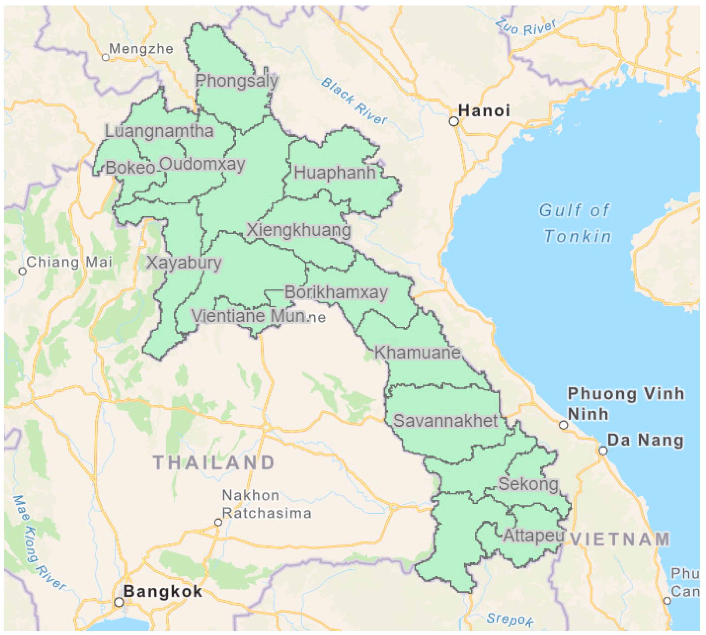
2.1. Overview of Study Area and Definition of Solid Waste in Laos

The area of study is chosen as the urban region of Laos. Laos is a small landlocked lower-middle-income nation situated in the center of Southeast Asia which covers an area of 236,800 km². It is surrounded by Cambodia, China, Vietnam and Thailand. Administratively, it consists of seventeen provinces which are further divided into villages, urban towns, and one capital city Vientiane [18]. Figure 1 shows the map of Laos. Geographically it is a leading rural country but the growing urbanization is the major cause of increasing solid waste and its related problems in the country. The solid waste in Laos is defined as the objects, chemical substances or any things that persons or legal entities do not want and cannot recycle such as used oil, rubbish, wastewater and others, which are toxic or non-toxic and categorizes into two types: general waste and toxic and hazardous wastes. General waste consists of organics, paper, plastics, glass, cans and other metal whereas hazardous waste refers to batteries, old paint cans, aerosols, chemical bottles and other refuse [19].

2.2. Multi-Linear Regression

The multi-linear regression approach is a methodology where the dependent variables are correlated to more than two independent variables to obtain a quantitative and qualitative relation between them. The mathematical presentation of the MLR approach is as follows:

Y = bₒ + b₁X₁ + b₂X₂ + b₃X₃ +...….….+ bₙXₙ + ε

(1)

Y signifies the dependent variable or to be forecasted or predicted variable, bₒ is the constant term X₁, X₂, X₃, Xₙ are the independent variables, b₁, b₂, b₃, bₙ are the regression coefficients of their respective independent variables and ε is the residual error which is assumed to be independent and identically distributed with zero mean and constant variance [20]. The value of the regression coefficients can be positive or negative where the positive value signifies the direct relation and the negative value signifies the indirect relation of the independent variable with the dependent variable. The numerical value of the coefficients denotes the one unit change of the value of the dependent variable with the respective independent variable.

2.3. Variable Selection

The dependent variable is the outcome variable of this study which is the solid waste generation rate in the urban region of Laos (SWGR). In total, six independent variables are selected for this study. They are urban population, per capita GDP, urban literacy rate, urban poverty incidence, urban household size and urban unemployment rate. Here, the study chooses the independent variables based on the availability of their reliable and comparable official statistics because sometimes it is difficult to obtain reliable data statistics for the desired SDE factors [17]. Nevertheless, many studies have proved that population and solid waste generation rates are directly proportional to each other [21]. The income of a person plays a key role in affecting the solid waste generation amount in any region [22] and here GDP per capita is used as a substitute for “income per capita” due to its non-availability for the official data. Other commonly used independent variables used for this study are literacy rate and household size, which can have both direct as well as indirect effects on SWGR depending on the region [23]. The household size signifies the average number of people living in one house; it is assumed that more people generate more waste [13] but more people can also utilize the same things, i.e., reusing or recycling waste happens in a big family which results in the decrease of solid waste [11]. The literate people are assumed to be knowledgeable or aware of waste management which affects the generation amount. In Laos, overall the poverty ratio has decreased to 23.2% from 33.5% in the past ten years [24]. The decreasing poverty rate increases the quality of life which affects the amount of solid waste [25]. The last independent variable chosen for this study affecting the amount of SWGR is the unemployment rate which is an indirect indication of the economic condition of any country or its region [26]. It is proved as another indicator affecting solid waste.

Table 1. A detailed description of all variables.

Type	Variable Name	Type	Description
Dependent Variable (DV)	Urban Solid Waste Generation Rates (SWGR)	Ton per year (TPY)	It is defined as the rate of generation of solid waste in the urban region.
Independent Variable (IV)	Gross Domestic Product (GDP) per capita	Current United States Dollars (USD)	It is defined as gross domestic product divided by midyear population. Gross domestic product is the sum of gross value added by all resident producers in the economy plus any product taxes and minus any subsidies not included in the value of the products.
Independent Variable	Urban Population (Population/Pop)	People	It is defined as the population living in the urban areas as defined by the national statistical offices of respective countries.
Independent Variable	Urban Literacy Rate (Literacy Rate/LR)	Percent (%)	It is defined as the rate of urban population to have the ability to identify, understand, interpret, create, communicate and compute, use printed and written materials associated with varying contexts. Here population aged 15 years and above is considered with literacy rates in the urban region of Laos.
Independent Variable	Urban Poverty Incidence (Poverty Incidence/PI)	Percent (%)	It is defined as the percentage of the urban population living below the national poverty lines (Source: World Bank). National estimates are based on population-weighted subgroup estimates from household surveys (Source: Census of Laos).
Independent Variable	Urban Household Size (Household Size/HS)	People Per Household (PPH)	It is defined as a household/social unit consisting of one or more persons who live together under the same roof and make common arrangements in the provision of food and other living conditions for themselves irrespective of blood relation or marriage in urban areas.
Independent Variable	Urban Unemployment Rate (Unemployment Rate/UR)	Percent (%)	It is defined as the rate at which the urban population is without work, currently available for work, seeking work in the recent past period, people who lost their jobs and includes people who voluntarily left their job.

Source: World Bank and Census of Laos.

provides a detailed description of all the variables selected for this study.

2.4. Data Collection

2.4.1. Data Collection for the Independent Variables

Here, the model is developed for predicting the SWGR for the urban region of Laos using SDE factors with the MLR approach. The reasonable way of choosing the value of independent variables is their availability with time. To perform this study, the priority for the data selection is given to the national reports or official and published documents. The second priority for choosing the data is given to the official reports or data organizations such as World Bank, ADB (Asian Development Bank), JICA (Japan International Cooperation Agency), etc. In the case of the unavailability of the mentioned data sources, the data is obtained from the secondary literature. The World Bank provided the data for the urban population from the year 1995 to 2050 and GDP per capita in Laos from the year 1995 to 2018 [27]. Census of Laos provided the data for literacy rate, household size and the unemployment rate for the year 1995 [28], 2005 [29] and 2015 [30]. The data for the poverty incidence is adopted from a secondary reference for the years 1992, 1997, 2002, 2007 and 2012 [31]. Unfortunately, reliable data is available for all independent variables is for the short time range, i.e., 1995 to 2012. The small data sets are very difficult to study in the MLR approach and they can also result in the wrong interpretation of statistical tests [32]. To overcome this difficulty, the time range selected to enter the historical values was chosen from the year 1995 to the year 2015.

2.4.2. Data Collection for the Dependent Variable

In the year 1992, JICA reported the SWGR as 0.63 kg (kilogram)/capita/day in Vientiane [33]. Later in the year 2005 Khanal et al. [34] reported 0.70 kg/capita/day of solid waste for Vientiane capital city, Glawe et al. [35] reported 0.75 kg/capita/day of waste for Laos in the year 2006, Shekdar [36] reported 0.70 kg/capita/day waste for Laos in the year 2009; UNEP (United Nations Environment Program) [37] reported 0.30 kg/capita/day to 0.70 kg/capita/day of waste in the year 2010 for the least developed countries including Laos and IGES (Institute for Global Environmental Strategies) [38] reported on average 0.60 to 0.70 kg/capita/day waste generation for all cities in Laos in the year 2012. The country analysis report in Laos reported 0.75 kg/capita/day of waste in the year 2013 [39] and 2015 CCAC (Climate and Clean Air Coalition) reported 0.65 kg/capita/day of waste for Vientiane [40]. Unfortunately, it is found that there are very limited studies that exist for Laos which show reliable SWGR statistics, especially for the urban region. Moreover, the available data in these references are inconsistent. The only concern of the MLR approach is obtaining false results in the case of using and analyzing improper and incomplete data. To obtain the accurate results for the predictive model, the study has adopted the data for the dependent variable from the recent national report prepared by MONRE (Ministry of Natural Resources and Environment) in the year 2017 which shows that the urban region generated 0.65 kg of waste in the year 2000 and 0.69 kg of waste in the year 2011 on a per capita per-day basis [3]. The daily per capita urban SWGR is estimated as 0.40 kg in 1990, using a secondary reference [41]. The missing data for the urban per capita SWGR is also interpolated and extrapolated (using the same increasing trends from the past) using MS Excel.

3. Results

The results are obtained for the best predictive model to evaluate the SWGR in the urban region of Laos using the multi-linear regression approach. The study prepares the model by assuming that the present trends of solid waste generation rates will remain the same in the future. To do so, different reliable models are generated in different scenarios in “IBM SPSS Statistics Version 25”. The MLR method provides statistically significant or valid results on the condition of satisfying its theory of key and necessary assumptions. It is the first step to know whether the data set can be analyzed using the MLR process or not. The major assumptions of MLR concern checking linearity, normality, multi-collinearity, homoscedasticity and autocorrelation. The violation of these assumptions often results in inaccuracy and imprecision of the developed model because of the generation of error terms related to both DV and IV. In total, results for seven models are presented which are created under four different scenarios for this study. The ability to provide accurate results is indicated by the value of MAE, RMSE and MAPE.

To perform the MLR, all the available dependent and the independent variables were entered in the software in different rows. The missing or unavailable data for the remaining year was interpolated or extrapolated using MS-Excel, 2016 (Microsoft-Excel). The extrapolation is used to create the data for poverty incidence for the years 2013, 2014 and 2015 based on its previous increasing and decreasing trend. The historical values entered for DV and IV are from the year 1995 to the year 2015. The real data is available for per capita solid waste generation rate for the urban region of Laos. The total urban SWGR is calculated in ton per year (TPY) by multiplying the per capita SWGR and population with the factor of 365/1000: SWGR = per capita SWGR*population*365/1000.

Table 2. Data for all variables entered into the SPSS software.

Type	Dependent Variable	Independent Variables
Year	SWGR (TPY)	GDP per capita (USD)	Population (People)	Literacy Rate (%)	Poverty Incidence (%)	Household Size (PPH)	Unemployment Rate (%)
1995	161,391	364	842,222	76.60	23.86	6.00	4.50
1996	181,237	378	902,801	77.87	22.98	5.94	4.46
1997	202,659	346	965,620	79.14	22.10	5.88	4.42
1998	225,773	249	1,030,927	80.41	21.62	5.82	4.38
1999	250,698	278	1,098,951	81.68	21.14	5.76	4.34
2000	277,580	325	1,169,990	82.95	20.66	5.70	4.30
2001	296,748	327	1,243,825	84.22	20.18	5.64	4.26
2002	316,865	320	1,320,796	85.49	19.70	5.58	4.22
2003	338,011	363	1,401,187	86.76	19.24	5.52	4.18
2004	360,413	418	1,485,877	88.03	18.78	5.46	4.14
2005	381,353	476	1,563,651	89.30	18.32	5.40	4.10
2006	397,778	591	1,622,169	89.72	17.86	5.35	4.06
2007	415,020	710	1,683,371	90.14	17.40	5.30	4.02
2008	433,038	900	1,747,050	90.56	15.92	5.25	3.98
2009	451,619	949	1,812,307	90.98	14.44	5.20	3.94
2010	470,669	1141	1,878,749	91.40	12.96	5.15	3.90
2011	490,141	1378	1,946,164	91.82	11.48	5.10	3.86
2012	510,106	1581	2,014,818	92.24	10.00	5.05	3.82
2013	530,602	1826	2,084,844	92.66	8.52	5.00	3.78
2014	551,844	1998	2,157,058	93.08	7.04	4.95	3.74
2015	573,944	2135	2,231,865	93.50	5.56	4.90	3.70

shows the data for all the variables which were entered into the software for running the MLR.

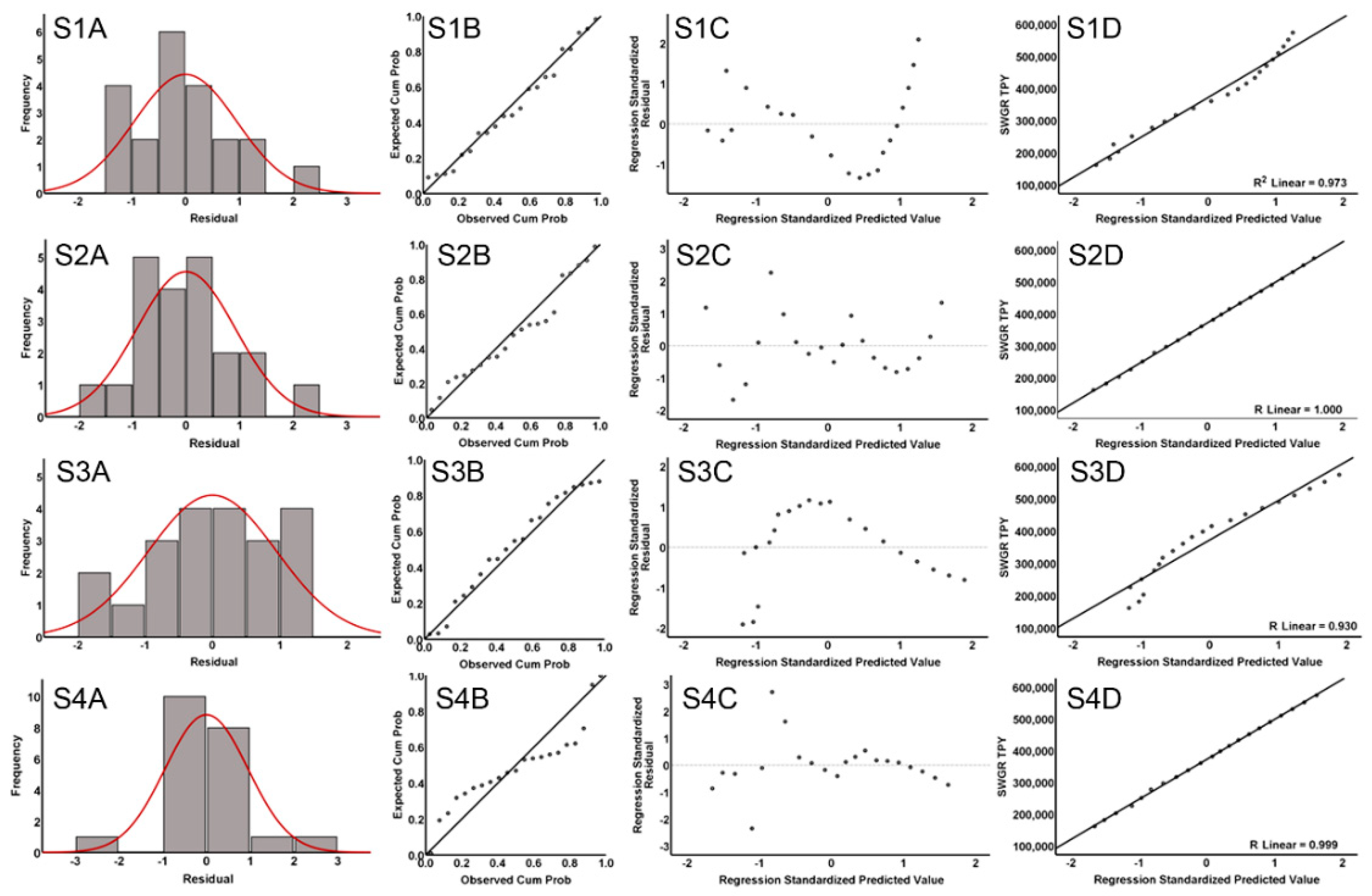
3.1. Model Assumptions

The linearity is checked by plotting the scatterplots. The normality of the dependent and independent variables is checked descriptively by obtaining the non-parametric matrix which is a one-sample Kolmogorov–Smirnov test (

Table 3. Test summary for one-sample Kolmogorov–Smirnov test for all variables.

Hypothesis Test Summary: One-Sample Kolmogorov-Smirnov Test
Type of Variable/Statistics	DV	IV						TV
	SWGR	GDP	Pop	LR	PI	HS	UR	InvGDP
Mean	372,261.38	812.05	1,533,535.33	87.07	16.66	5.43	4.10	0.00
Standard Deviation	126,122.758	619.813	434,560.633	5.407	5.440	0.342	0.248	0.001
Significant number	0.200 1,2	0.05 1	0.200 1,2	0.063 1	0.0991	0.200 1,2	0.200 1,2	0.200 1,2
Decision for the null hypothesis	Retain	Reject	Retain	Retain	Retain	Retain	Retain	Retain

Asymptotic significances are displayed. The significance level is 0.05. ¹ Lilliefors Corrected. ² This is a lower bound of the true significance.

) along with a z-test by obtaining the skewness and Kurtosis value (

Table 4. Normality descriptive for dependent, independent and transformed variables.

Type of Variable/Statistics	DV	IV						TV
	SWGR	GDP	Pop	LR	PI	HS	UR	InvGDP
Skewness Statistics (SS)	−0.101	1.055	−0.033	−0.641	−0.727	0.127	0.000	0.085
Standard Error-Skewness (SES)	0.501	0.501	0.501	0.501	0.501	0.501	0.501	0.0501
ZS	−0.201	2.105	−0.066	−1.280	−1.450	0.253	0.000	0.170
Kurtosis Statistics (KS)	−1.115	−0.251	−1.229	−0.946	−0.600	−1.191	−1.200	−1.424
Standard Error Kurtosis (SEK)	0.972	0.972	0.972	0.972	0.972	0.972	0.972	0.972
ZK	−1.147	−0.258	−1.264	−0.973	−0.617	−1.225	−1.235	−1.465

). The non-parametric tests result in the rejection or retaining of the null hypothesis of variables and are preferred for small data sets [42]. The z-test signifies the passing or failing of the normality hypothesis which is evaluated by calculating the z-score of skewness (Zs) and z-score of Kurtosis (Zk) whose value range is ±1.96 [43]. According to Table 4, the value of Zs, Zk is greater than 1.96 which rejects the null hypothesis of normality for GDP which is computed to be normal using inverse transformation (IT).

IT is a commonly used transformation for positively skewed variables among IT (1/x), log transformations (ln or log10), cubic root transformations (x^1/3) and square root transformation (x²). The best way for choosing the transformation is by testing “which fits the best”. The study has one transformed variable, i.e., GDP which is denoted as “InvGDP”. The normality descriptive for dependent, independent and transformed variables are shown in Table 4.

Table 5. Results of correlation-matrix for four scenarios prepared in the study.

Scenario	Model	Included IV	Unstandardized Beta Coefficients	p-Value	VIF	Tolerance	Comments
Scenario 1		Constant	−1,116,300.616	0.000
		InvGDP	−27,956,844.271	0.003	3.759	0.266
		Literacy Rate	17,728.688	0.000	3.759	0.266
Scenario 2	Model 1	Constant	2,374,879.277	0.000
		Household Size	−369,065.167	0.000	1.000	1.000
	Model 2	Constant	2,303,206.560	0.000			Presence of multi-collinearity
		Household Size	−352,509.475	0.000	10.980	0.091
		Poverty Incidence	−1090.445	0.012	10.980	0.091
	Model 3	Constant	1,169,994.593	0.002			Presence of multi-collinearity
		Household Size	−219,017.073	0.000	652.847	0.002
		Poverty Incidence	−4433.539	0.000	113.071	0.009
		Literacy Rate	5334.977	0.002	256.856	0.004
Scenario 3		Constant	709,656.153	0.000
		InvGDP	−28,081,498.413	0.079	4.812	0.208
		Poverty Incidence	−16,932.000	0.000	4.812	0.208
Scenario 4	Model 1	Constant	−72,478.318	0.000
		Population	0.290	0.000	1.000	1.000
	Model 2	Constant	−120,245.001	0.000
		Population	0.310	0.000	6.344	0.158
		InvGDP	8,406,640.193	0.000	6.344	0.158
Dependent variable: SWGR

shows the result of the correlation matrix showing the value for beta coefficient, tolerance value, VIF value and p-value for all the models of different scenarios. Scenario1 is performed using the “enter” method and resulted in a high VIF value and low tolerance value for the independent variables. The VIF value and tolerance value define the strength of correlation among the independent variables and are reciprocal to each other (VIF = 1/Tolerance or Tolerance = 1/VIF). The high value of VIF indicates the issue of multi-collinearity in the model. The presence of multi-collinearity jeopardizes the strength of the quantitative relationship between the dependent and the independent variable by poorly estimating the value of beta coefficients. The removal of multi-collinearity assures fewer standard errors and uncertainty in the value of regression coefficients and verifies the validity of the model. The process of removing this issue deals with the removal of independent variables from the model in a cascade manner until the VIF value obtained for IV is less than 10. A VIF value greater than 10 indicates high collinearity among the variables [44].

Scenario 2 provides three models which are resulted from using the “stepwise” method. SPSS has five methods for running the MLR which are enter, stepwise, remove, backward (elimination) and forward (selection). The enter method includes all the independent variables in a single step and forms the regression equation, whereas in the remove method all the entered variables are removed concurrently from the model. The stepwise method includes variables in step-by-step manners and prepares the model by adding or removing the independent variables in progression by checking the statistical significance after each step. All methods are performed in Scenario 2 where the stepwise method and forward method resulted in the development of the same models but the backward method and remove method showed the issue of multi-collinearity with a much higher value for VIF. Table 5 only presents the model results obtained from the stepwise method in Scenario 2. The advantage of using the stepwise approach over the forward, backward and remove method is because it adds the variable at two significance levels: adding variables or removing variables. Moreover, the stepwise method is a combination of the forward method and the backward method [45], as the forward method performs step-up selection and the backward method performs a step-down selection of variables. In total three models are obtained in this approach. Model 1 resulted in variable household sizes and showed VIF value equals to 1, Model 2 includes household size and poverty incidence with a VIF value of 10.980 for both variables, and Model 3 resulted in household size, poverty incidence and literacy rate with a VIF value greater than 10 for each variable; this signifies the issue of multi-collinearity.

The other method of removing the multi-collinearity is by manually removing the highly correlated variables based on the result of person correlation values. The bivariate matrix is presented in

Table 6. Results of bivariate-matrix for dependent and the (transformed) independent variables.

		InvGDP	Pop	PI	HS	UR	SWGR
InvGDP	Pearson Correlation	1	−0.918 **	0.890 **	0.909 **	0.916 **	−0.905 **
	Sig. (2-tailed)		0.000	0.000	0.000	0.000	0.000
Pop	Pearson Correlation	−0.918 **	1	−0.961 **	−0.999 **	−1.000 **	0.999 **
	Sig. (2-tailed)	0.000		0.000	0.000	0.000	0.000
PI	Pearson Correlation	0.890 **	−0.961 **	1	0.953 **	0.965 **	−0.957 **
	Sig. (2-tailed)	0.000	0.000		0.000	0.000	0.000
HS	Pearson Correlation	0.909 **	−0.999 **	0.953 **	1	0.999 **	−1.000 **
	Sig. (2-tailed)	0.000	0.000	0.000		0.000	0.000
UR	Pearson Correlation	0.916 **	−1.000 **	0.965 **	0.999 **	1	−0.999 **
	Sig. (2-tailed)	0.000	0.000	0.000	0.000		0.000
SWGR	Pearson Correlation	−0.905 **	0.999 **	−0.957 **	−1.000 **	−0.999 **	1
	Sig. (2-tailed)	0.000	0.000	0.000	0.000	0.000

Correlation is significant at the 0.01 level (2-tailed) **.

, which indicates the high correlation among the population, literacy rate, household size and unemployment rate. Scenario 3 and Scenario 4 are the results of manual selection of the variables population, InvGDP and poverty incidence for developing the final models. The population is selected as a key indicator among all because many studies have proved that its direct effect on the amount of solid waste generation rates. Scenario 3 is a result of the enter method, where the model includes InvGDP and poverty incidence with a VIF value of 4.812 for both variables. Scenario 4 is a result of stepwise regression. It consists of two models where Model 1 includes population and Model 2 includes population and InvGDP with a VIF value of 6.344.

Table 7. Results of model summary and ANOVA matrix for all scenarios.

Scenarios		Scenario 1	Scenario 2			Scenario 3	Scenario 4
			Model 1	Model 2	Model 3		Model 1	Model 2
Predictors (DV: SWGR)		InvGDP, LR	HS	HS, PI	HS, PI, LR	InvGDP, PI	Pop	Pop, InvGDP
Model Summary	R square (R2)	0.973	0.999	1.000	1.000	0.930	0.998	0.999
	Adjusted R square	0.970	0.999	0.999	1.000	0.922	0.998	0.999
	Standard Error of Estimate	21,899.392	3356.025	2885.686	2237.220	35,171.722	5049.880	3268.159
	Durbin Watson Factor	0.278	1.022			0.154	1.179
ANOVA	F	322.683	28,227.611	19,093.433355	21,181.759745	119.588	12,456.408	14,883.936
	Sig.	0.000	0.000	0.000	0.000	0.000	0.000	0.000

provides the result of the model summary and analysis of variance ANOVA matrix for all scenarios. The same value of R² and adjusted R² shows no change in the model with the addition of new values. It also happens when there is only one variable in the model. The lower value of adjusted R² than R² shows that model has not improved with the addition of a new variable. The difference in the values of R² and adjusted R² increases with the addition of non-significant variables to the model. The value closer to 1 signifies the perfect prediction of the model [46]. The other statistical parameters are also shown in Table 7, i.e., standard error of estimates, F and p-value in ANOVA matrix. The significance level is checked at an alpha (α) value of 0.05; the value lower than 0.05 proves the statistical significance of the model. The hypothesis of auto-correlation (error terms are independent of each other) is checked by estimating the Durbin Watson Factor (DWF) at a significance level of 0.05. Statistically, the value of DWF lies between 0 to 4. The value closer to 1 or between 0 to 2 indicates a positive correlation and the value between 2 to 4 indicates a negative correlation among the input variables.

The validity of the prepared model in MLR is assured by the distribution of variances in the model. It is often suggested that verifying the assumption of homoscedasticity or testing the normality of the residuals (the difference between the observed value of the dependent variable and predicted value) is significant for generating the valid model. The non-satisfaction of the assumption of normality of residuals challenges the validity and indicates an inadequacy in the developed model. Figure 2 shows the histogram, p–p (probability–probability) plots, residual plots and scatter plots for the dependent variable for four scenarios. The approximate lying of observation on the straight line in the p–p plot shows the normal distribution of residuals and confirms the validity of the model. Descriptively the normality of residual errors or homoscedasticity is checked by the popular Breusch–Pagan test or White-test. The power issue of the tests could lead to false or unsatisfying results for small sample data sets [47]. It is also difficult to state whether the assumption of homoscedasticity is passed or failed by looking at the graphs with small datasets. Here to check the normal distribution of the residuals, the square of residuals was evaluated with each model and analyzed with their respective independent variables in a linear regression option at a significance level of 0.05.

Table 8. Results of homoscedasticity for all scenarios.

Scenario	Scenario 1	Scenario 2			Scenario 3	Scenario 4
		Model 1	Model 2	Model 3		Model 1	Model 2
Predictor variables	InvGDP, LR	HS	HS, PI	HS, PI, LR	InvGDP, PI	Pop	Pop, InvGDP
p-value	0.179	0.128	0.544	0.291	0.006	0.001	0.062
Result (Homoscedasticity (Pass)/Heteroscedasticity (Fail))	Pass	Pass	Pass	Pass	Fail	Fail	Pass

shows the result of the assumption of homoscedasticity. A significant value greater than 0.05 in the ANOVA (analysis of variance) matrix indicates the passing of the null hypothesis of normality and states that the residuals of the error terms are normally distributed.

3.2. Model Accuracy and Validity

To check the accuracy and validity of the developed model popular key performance indicators (KPI) such as mean absolute error (MAE), root mean square error (RMSE) and mean absolute percentage error (MAPE) are evaluated by using the following equations.

$$\begin{gathered} \mathrm{MAE}=\frac{{{\displaystyle \sum }}_{\mathrm{t}=1}^{\mathrm{n}}\mathrm{ABS}\left(\mathrm{At}-\mathrm{Pt}\right)}{\mathrm{n}} \\ \mathrm{RMSE}=\sqrt{\frac{{{\displaystyle \sum }}_{\mathrm{t}=1}^{\mathrm{n}}\left(\mathrm{At}-\mathrm{Pt}\right)^2}{\mathrm{n}}} \\ \mathrm{MAPE}=\frac{{{\displaystyle \sum }}_{\mathrm{t}=1}^{\mathrm{n}}\mathrm{ABS}\left(\frac{\mathrm{At}-\mathrm{Pt}}{\mathrm{At}}\right)}{\mathrm{n}}\times 100 \end{gathered}$$

where, “At” denotes the original or actual data at time t, “Pt” denotes the predicted data at time t, “n” denotes the total number of terms of data points. The indicators are calculated using MS-Excel, 2016. MAE tells the variability in the dataset by evaluating the average distance between each data value and the mean. This method is often used to check the accuracy of predicted values when the units are the same for the original and predicted data. RMSE is an independent measure of fit and is estimated by taking the square root of the averaged square difference between the predicted data and the original data. The squaring of errors in RMSE always gives positive results. Both MAE and RMSE share similarities for their working on the principle that “smaller the error the better the prediction ability”. Numerically, RMSE is always greater than or equal to MAE. The estimated values for MAE and RMSE depend on the range of the data and the range of estimation could vary from 0 to ∞. MAPE is another popular and frequently used PVI for measuring the accuracy of predictive models due to its scale-independency and easy interpretability. It takes the average of absolute percentage errors of prediction. The lower value of MAE, RMSE and MAPE indicates better and accurate prediction. The MAPE is limited to provide results for only non-zero values. The table below provides the estimated values for MAE, RMSE and MAPE.

Table 9. Values of key performance indicators for all scenarios.

PVI	Scenario 1	Scenario 2			Scenario 3	Scenario 4
		Model 1	Model 2	Model 3		Model 1	Model 2
	InvGDP, LR	HS	HS, PI	HS, PI, LR	InvGDP, PI	Pop
MAE	16,557.18	2575.75	2293.16	1552.92	26,523.45	3475.04	1886.40
RMSE	20,278.68	3192.27	2671.62	2012.86	32,571.25	4803.40	3030.74
MAPE	4.49	0.71	0.72	0.53	9.35	1.36	0.67

shows the results of performance indicators obtained for the MAE, RMSE and MAPE.

The best model is evaluated based on the results obtained in Table 7 and Table 9. The values obtained for the PVI are compared numerically where Model 3 of Scenario 2 shows the least values for MAE, MSE, RMSE and MAPE. However, it is not used as a predictive model because of the presence of high multi-collinearity. Scenario1 and Model 2 of Scenario 2 are rejected due to the high value of MAPE and the presence of multi-collinearity respectively. Model 1 of Scenario 4 is not considered the best model because it rejects the assumption of homoscedasticity which indicated the absence of normality of residual errors. Scenario 3 failed the test of normality of residual errors, i.e., homoscedasticity and also resulted in a high value of MAPE. Model 1 of Scenario 2 and Model 2 of Scenario 4 passed the assumptions of MLR for multi-collinearity, normality and homoscedasticity. The significance values obtained in the ANOVA matrix to test the assumption only indicate the absence or presence of homoscedasticity. It should be noted that these values obtained for PVI are lower for Model 2 of Scenario 4 which makes it a better predictive model among all the developed models. The final predictive equation from Model 2 of Scenario 4 is written by using the beta coefficients from Table 5 The positive sign for the beta coefficient of both variables signifies the direct relation of population and GDP per capita with the urban solid waste generation rates. The final generated equation is given as:

SWGR = (−120,245.001) + (0.310) × Population + (8,406,640.193) × InvGDP

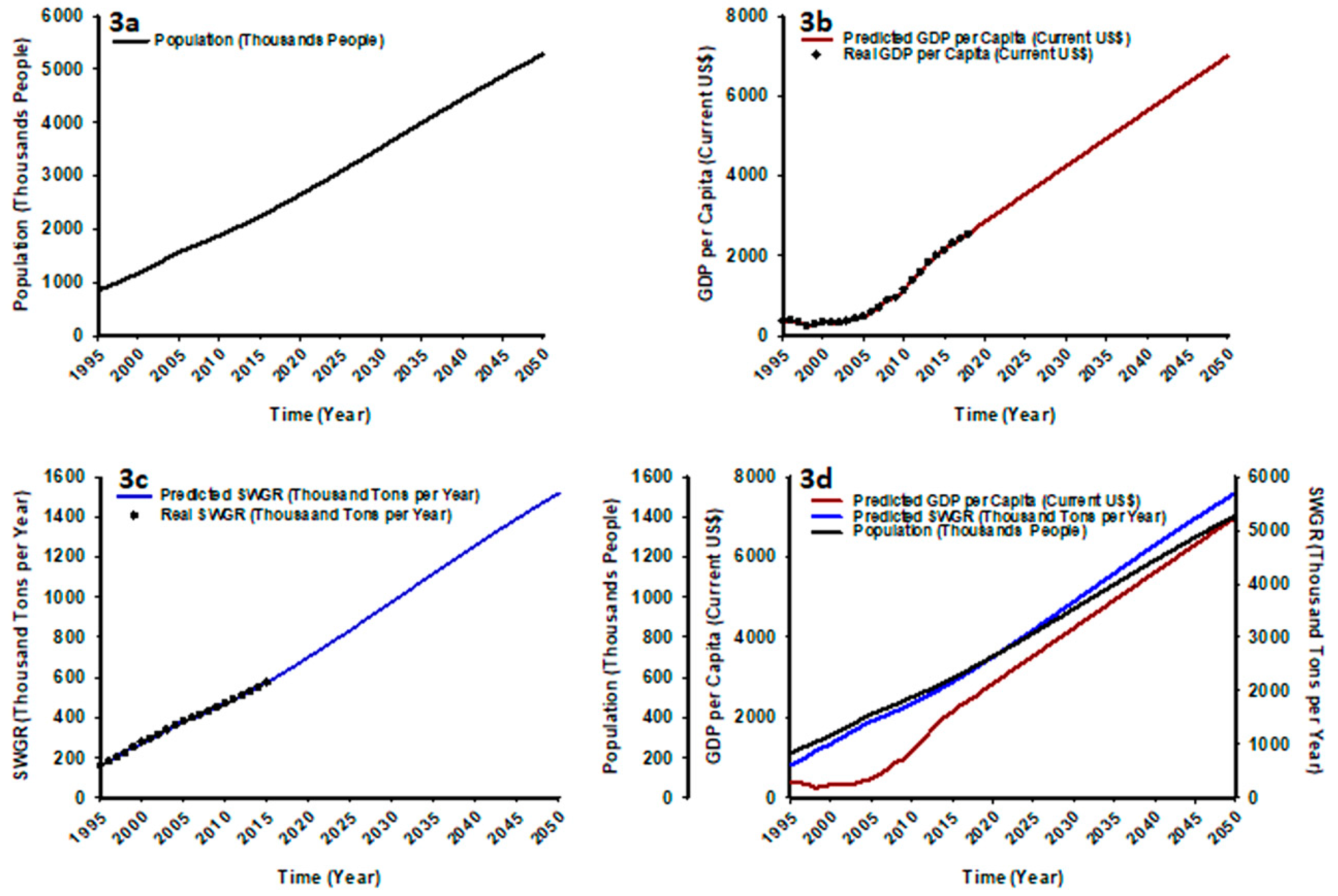
3.3. SWGR Prediction from 1995 to 2050

It is equally necessary to have accurate and official data for the independent variables to generate the predicted values after generating their mathematical relationship with the dependent variable or output variable to get accurate and reliable results. Here, Figure 3a shows the available and predicted data for the population adopted by the World Bank. Figure 3b presents the original and predicted data for GDP per capita in Laos which is forecasted for this study using MS-Excel 2016 by generating the forecast sheet. Figure 3c presents the original and forecasted results of solid waste generation rates in the urban region of Laos and Figure 3d shows the combined results of Figure 3a–c.

Figure 3d shows an increasing trend in the SWGR with the increasing population and increasing GDP. The urban solid waste generation rate of Laos will reach 0.98 million tons (MT) in the year 2030, 1.26 MT in the year 2040 and 1.52 MT in the year 2050. The per capita SWGR for the urban region of Laos is estimated to be 0.74 kg in the year 2030, 0.75 kg in the year 2040 and 0.76 kg in the year 2050 on daily basis. The average rate of growth for per capita solid waste generation rate is estimated to be around 17% from the year 2020 to 2050. The increasing urban population and increasing GDP per capita will tend to increase the total amount of solid waste in the urban region of Laos.

4. Discussion

The existing solid waste management system in Laos is inefficient and fruitless. Currently, at the national level, five major ministries are working for the management of solid waste in the country, i.e., MPWT (Ministry of Public Works and Transport), MONRE, MOIC (Ministry of Industry and Commerce), MOH (Ministry of Health), MAF (Ministry of Agriculture and Forestry) and MEM (Ministry of Energy and Mines). The MPWT supports and provides the technical guidelines and advice on planning, designing and management of SW infrastructure, the MOIC manages the industrial and hazardous waste, MOH manages the hospital and health sector waste and MAF manages the compost made from the household. The MONRE was established in the year 2011 to provide the regulatory framework for SWM, developing the strategies, policies and guidelines for SWM in the country. There are three reports prepared by MONRE in the year 2015 [48], 2016 [49] and 2017 [3] mentioning the need to manage the solid waste in Laos. Moreover, there is no separate document prepared at the central and local levels regarding any policy for managing the SW in the country.

The lack of reliable statistics is the biggest disadvantage and acts as a barrier to proper solid waste management in any country [1]. It is very challenging for the local government or policymakers to draw any useful conclusion for the proper handling or management of solid waste without any related and informative statistics of solid waste [6,11]. This study prepared the predictive model with the ability to predict the data for the past, present and future years. Different models are generated under different scenarios using the multi-linear regression (MLR) approach. The urban solid waste generation rate is correlated to six independent socio-demographic and economic parameters. The population and GDP per capita were found to be most effective for developing a predictive model for urban SWGR in Laos. It is found that the growing urban population and growing economy will lead to an increase in the amount of SWGR in the urban region of Laos. The SWGR will reach 0.98 Mt in the year 2030 with a 3.50 million population and USD (United States Dollar) 4229 of GDP per capita. This amount of waste generation for the urban region will increase to 1.5 Mt in the year 2050 with 5.2 million of population and GDP per capita of USD 6998. The validity and accuracy of the model are estimated by the value of R square, adjusted R square with key performance indicators, i.e., MAE, RMSE and MAPE. Among seven models of four scenarios, Model 2 of Scenario 4 is predicted as the best model with R² value as 0.999, adjusted R² as 0.999, MAE value as 1886.40, RMSE value as 3030.74 and MAPE value as 0.67. Moreover, this study also shows the predicted results for the input variables, i.e., population and GDP per capita up to the year 2050.

The study highlights the implications in the context of developing countries. The need for peaceful waste management is required in this region of the world, as they are trying to be at par with the developed nations. The implication of these simple steps could be magnified in processing and developing the waste system in this country. The trial of estimation of these factors for future waste generation may indeed beneficial for the government to make a sustainable waste management policy.

5. Conclusions

The predicted data for urban population, GDP per capita and urban solid waste generation rates will help the policymakers and the government to create a proper sustainable solid waste management policy in the country. It also provides future scope for researchers working on solid waste management in Laos. The easy explanation of the work will urge the researchers to use this technique for developing the solid waste management database in developing countries. The limitation of this study is the non-availability of enough data for developing the model. In the future, a large dataset and a wide range of socio-demographic and economic parameters can be considered to further improve the scope of the methodology and developed models.

References

1. Ferronato, N.; Torretta, V. Waste mismanagement in developing countries: A review of global issues. Int. J. Environ. Res. Public Health 2019, 16, 1060. [Google Scholar] [CrossRef] [PubMed] [Green Version]
2. Alessandra, G.; Dicma, B.; Garfí, M. Waste Disposal in Developing Countries and Emergency Situations. The Case of Saharawi Refugees Camps. Available online: https://www.iswa.org/uploads/tx_iswaknowledgebase/15-384paper_long.pdf (accessed on 8 February 2021).
3. MONRE. National Pollution Control Strategy and Action Plan. 2017. Available online: http://www.gms-eoc.org/uploads/resources/922/attachment/Laos-Pollution-Strategy-Plan-2018-2025-draft.pdf (accessed on 18 November 2020).
4. Chen, H.W.; Chang, N. Bin Prediction analysis of solid waste generation based on grey fuzzy dynamic modeling. Resour. Conserv. Recycl. 2000, 29, 1–18. [Google Scholar] [CrossRef]
5. Popli, K.; Luckman Sudibya, G.; Kim, S. A Review of Solid Waste Management using System Dynamics Modeling. J. Environ. Sci. Int. 2017, 1185–1200. [Google Scholar] [CrossRef]
6. Abbasi, M.; El Hanandeh, A. Forecasting municipal solid waste generation using artificial intelligence modelling approaches. Waste Manag. 2016, 56, 13–22. [Google Scholar] [CrossRef] [PubMed]
7. Intharathirat, R.; Abdul Salam, P.; Kumar, S.; Untong, A. Forecasting of municipal solid waste quantity in a developing country using multivariate grey models. Waste Manag. 2015, 39, 3–14. [Google Scholar] [CrossRef]
8. Al-Salem, S.M.; Al-Nasser, A.; Al-Dhafeeri, A.T. Multi-variable regression analysis for the solid waste generation in the State of Kuwait. Process Saf. Environ. Prot. 2018, 119, 172–180. [Google Scholar] [CrossRef]
9. Kolekar, K.A.; Hazra, T.; Chakrabarty, S.N. A review on prediction of municipal solid waste generation models. Procedia Environ. Sci. 2016, 35, 238–244. [Google Scholar] [CrossRef]
10. Lakioti, E.N.; Moustakas, K.G.; Komilis, D.P.; Domopoulou, A.E.; Karayannis, V.G. Sustainable solid waste management: Socio-economic considerations. Chem. Eng. Trans. 2017, 56, 661–666. [Google Scholar] [CrossRef]
11. Suthar, S.; Singh, P. Household solid waste generation and composition in different family size and socio-economic groups: A case study. Sustain. Cities Soc. 2015, 14, 56–63. [Google Scholar] [CrossRef]
12. Vieira, V.H.A.d.M.; Matheus, D.R. The impact of socioeconomic factors on municipal solid waste generation in São Paulo, Brazil. Waste Manag. Res. 2018, 36, 79–85. [Google Scholar] [CrossRef] [PubMed] [Green Version]
13. Trang, P.T.T.; Dong, H.Q.; Toan, D.Q.; Hanh, N.T.X.; Thu, N.T. The Effects of Socio-economic Factors on Household Solid Waste Generation and Composition: A Case Study in Thu Dau Mot, Vietnam. Energy Procedia 2017, 107, 253–258. [Google Scholar] [CrossRef]
14. Hidalgo, J.; Amaya, J.; Jervis, F.; Moreira, C. Influence of Socio-Economic Factors on Household Solid Waste (HSW) Generation of the City of Guayaquil, Ecuador. In Proceedings of the Sixteen Laccei International Multi-Conference for Engineering, Education and Technology, Montego Bay, Jamaica, 24–26 July 2019. [Google Scholar] [CrossRef] [Green Version]
15. Buenrostro, O.; Bocco, G.; Vence, J. Forecasting generation of urban solid waste in developing countries—A case study in Mexico. J. Air Waste Manag. Assoc. 2001, 51, 86–93. [Google Scholar] [CrossRef] [Green Version]
16. Wei, Y.; Xue, Y.; Yin, J.; Ni, W. Prediction of municipal solid waste generation in china by multiple linear regression method. Int. J. Comput. Appl. 2013, 35, 136–140. [Google Scholar] [CrossRef]
17. Kumar, A.; Samadder, S.R. An empirical model for prediction of household solid waste generation rate—A case study of Dhanbad, India. Waste Manag. 2017, 68, 3–15. [Google Scholar] [CrossRef]
18. Asian Development Bank. Lao People’s Democratic Republic: Urban Development Sector Assessment, Strategy, and Road Map; Asian Development Bank: Mandaluyong, Philippines, 2012; ISBN 978-92-9092-872-0. [Google Scholar]
19. Assembly, N. Lao PDR Environmental Protection Law. 2012. Available online: http://extwprlegs1.fao.org/docs/pdf/lao151747.pdf (accessed on 18 November 2020).
20. NRB Chapter 8: Multiple Linear Regression Natural Resources Biometrics. Available online: https://milnepublishing.geneseo.edu/natural-resources-biometrics/chapter/chapter-8-multiple-linear-regression/ (accessed on 18 November 2020).
21. Popli, K.; Lim, J.; Kim, H.K.; Kim, Y.M.; Tuu, N.T.; Kim, S. Prediction of greenhouse gas emission from municipal solid waste for South Korea. Environ. Eng. Res. 2020, 25, 462–469. [Google Scholar] [CrossRef]
22. Sivakumar, K.; Sugirtharan, M. Impact of Family Income and Size on Per Capita Solid Waste. J. Sci. Univ. Kelaniya 2010, 5, 13–23. [Google Scholar] [CrossRef] [Green Version]
23. Monavari, S.M.; Omrani, G.A.; Karbassi, A.; Raof, F.F. The effects of socioeconomic parameters on household solid-waste generation and composition in developing countries (a case study: Ahvaz, Iran). Environ. Monit. Assess. 2012, 184, 1841–1846. [Google Scholar] [CrossRef] [PubMed]
24. The World Bank Group. Drivers of Poverty Reduction in Lao PDR. Available online: https://openknowledge.worldbank.org/handle/10986/2119 (accessed on 18 November 2020).
25. Ali, N.E.; Sion, H.C. Solid waste management in Asian countries: A review of solid waste minimisation (3′r) towards low carbon. IOP Conf. Ser. Earth Environ. Sci. 2014, 18. [Google Scholar] [CrossRef] [Green Version]
26. Liu, J.; Li, Q.; Gu, W.; Wang, C. The impact of consumption patterns on the generation of municipal solid waste in China: Evidences from provincial data. Int. J. Environ. Res. Public Health 2019, 16, 1717. [Google Scholar] [CrossRef] [Green Version]
27. World Bank World Bank Open Data Data. Available online: https://data.worldbank.org/ (accessed on 9 February 2021).
28. Centre, N.S.; SCP Laos of Lao PDR. Atlas of Laos. 1995. Available online: http://www.diva-portal.org/smash/get/diva2:818132/FULLTEXT01.pdf (accessed on 19 November 2020).
29. Laos Census. Results of Lao PDR. 2005. Available online: https://data.opendevelopmentmekong.net (accessed on 19 November 2020).
30. Lao PDR. The 4th Population and Housing Census (PHC). 2015. Available online: https://lao.unfpa.org/sites/default/files/pub-pdf/PHC-ENG-FNAL-WEB_0.pdf (accessed on 19 November 2020).
31. Warr, P.; Rasphone, S.; Menon, J. Two Decades of Declining Poverty Despite Rising Inequality in Laos. 2015. Available online: https://www.adb.org/sites/default/files/publication/176031/ewp-461.pdf (accessed on 19 November 2020).
32. Kiralj, R.; Ferreira, M.M.C. Basic validation procedures for regression models in QSAR and QSPR studies: Theory and application. J. Braz. Chem. Soc. 2009, 20, 770–787. [Google Scholar] [CrossRef] [Green Version]
33. JICA Present Solid Waste Management in Vientiane 1992. Available online: https://openjicareport.jica.go.jp/pdf/11008042_02.pdf (accessed on 19 November 2020).
34. Khanal, B.R.; Souksavath, B. Environmental Management Measures and Current Practices in Solid Waste Management: A Case Study from Vientiane, Lao People’s Democratic Republic. J. GMS Dev. Stud. 2005, 2, 69–89. [Google Scholar]
35. Glawe, U.; Visvanathan, C.; Alamgir, M. Solid Waste Management in Least Developed Asian Countries—A Comparative Analysis. In Proceedings of the International Conference on Integrated Solid Waste Management in Southeast Asian Cities: Proceedings, Siem Reap, Cambodia, 5–7 July 2005; pp. 1–11. [Google Scholar]
36. Shekdar, A.V. Sustainable solid waste management: An integrated approach for Asian countries. Waste Manag. 2009, 29, 1438–1448. [Google Scholar] [CrossRef] [PubMed]
37. UNEP. MSW Management Report. 2010. Available online: http://www.rrcap.ait.ac.th/Publications/MW_status_quo.pdf (accessed on 20 November 2020).
38. IGES. A Guide for Improving Municipal Solid Waste Management and Promoting Urban Organic Waste Utilization in Lao PDR. 2012. Available online: https://www.iges.or.jp/en/pub/guide-improving-municipal-solid-waste/en (accessed on 6 March 2020).
39. MPWT; MONRE. Fourth Regional 3R Forum in Asia Brief Country Analysis Paper Lao PDR. 2013, pp. 18–20. Available online: https://www.uncrd.or.jp (accessed on 20 November 2020).
40. CCAC Solid Waste Management City Profile—Vientiane Capital. LAO People’s Democratic Republic, 2015.
41. STEA. Lao People’s Democratic Republic The First National Communication on Climate Change. 2000. Available online: https://unfccc.int/resource/docs/natc/laonc1.pdf (accessed on 23 November 2020).
42. Garth, A. Analysing data using SPSS (A practical guide for those unfortunate enough to have to actually do it). 2008. Available online: https://students.shu.ac.uk/lits/it/documents/pdf/analysing_data_using_spss.pdf (accessed on 20 November 2020).
43. Mishra, P.; Pandey, C.M.; Singh, U.; Gupta, A.; Sahu, C.; Keshri, A. Descriptive statistics and normality tests r statistical data. Ann. Card. Anaesth. 2019, 22, 67–72. [Google Scholar] [CrossRef]
44. Ferre, J. Regression Diagnostics. In Contemporary Sociology; Sage: Thousand Oaks, CA, USA, 2009; Volume 21, p. 548. [Google Scholar]
45. Lewis-Beck, M.; Bryman, A.; Futing Liao, T. Stepwise Regression. In The SAGE Encyclopedia of Social Science Research Methods; SAGE Publications, Inc.: Thousand Oaks, CA, USA, 2012; pp. 1–9. [Google Scholar]
46. Ratner, B. The correlation coefficient: Its values range between 1/1, or do they. J. Target. Meas. Anal. Mark. 2009, 17, 139–142. [Google Scholar] [CrossRef] [Green Version]
47. Li, Z.; Yao, J. Testing for heteroscedasticity in high-dimensional regressions. Econom. Stat. 2019, 9, 122–139. [Google Scholar] [CrossRef]
48. MONRE. MONRE Vision Toward 2030. 2015. Available online: http://extwprlegs1.fao.org/docs/pdf/lao170969.pdf (accessed on 20 November 2020).
49. MONRE. National Biodiversity Strategy and Action Plan 2016—2025. 2016. Available online: https://leap.unep.org/countries/la/national-legislation/national-biodiversity-strategy-and-action-plan-2016-2025 (accessed on 20 November 2020).
Figure 1. Map of Laos. Laos is a land-locked country surrounded by Cambodia, China, Vietnam and Thailand. It has seventeen provinces and one capital city Vientiane.
Sustainability 13 03038 g001
Figure 2. Histograms, p–p plots, residual plots and scatter plots for the dependent variable. S1A, S2A, S3A and S4A shows the histogram of residuals for the dependent variable for four scenarios respectively; S1B, S2B, S3B and S4B shows the normal p–p plot of observed cumulative probability of residuals of the dependent variable for four scenarios respectively; S1C, S2C, S3C and S4C shows regression standardized predicted value against regression standardized residuals of the dependent variable for four scenarios respectively and S1D, S2D, S3D and S4D shows the scatter plot of regression standardized predicted value against the dependent variable for four scenarios respectively.
Sustainability 13 03038 g002
Figure 3. Real and predicted data for the urban population, GDP per capita and urban solid waste generation rate (SWGR) in Laos. (a) Shows obtained data for the urban population of Laos from 1995 to 2050 (The predicted data for the urban population is provided by the World Bank). (b) Shows real data (1995 to 2018) and predicted data (2019 to 2050) of GDP per capita for Laos. The real data for GDP per capita is obtained from the World Bank from 1995 to 2018. (c) Shows real data (1995 to 2011) and predicted data (2012 to 2050) of urban SWGR for Laos. The real data for urban SWGR is obtained from MONRE, 2017. (d) Shows the combined result of (ac).
Sustainability 13 03038 g003