Machine Learning-Based Node Characterization for Smart Grid Demand Response Flexibility Assessment

Abstract

As energy distribution systems evolve from a traditional hierarchical load structure towards distributed smart grids, flexibility is increasingly investigated as both a key measure and core challenge of grid balancing. This paper contributes to the theoretical framework for quantifying network flexibility potential by introducing a machine learning based node characterization. In particular, artificial neural networks are considered for classification of historic demand data from several network substations. Performance of the resulting classifiers is evaluated with respect to clustering analysis and parameter space of the models considered, while the bootstrapping based statistical evaluation is reported in terms of mean confusion matrices. The resulting meta-models of individual nodes can be further utilized on a network level to mitigate the difficulties associated with identifying, implementing and actuating many small sources of energy flexibility, compared to the few large ones traditionally acknowledged.

1. Introduction

Safe and reliable operation of energy systems depends on maintaining a balance between consumption and production in real-time, while an increasingly large part of the production portfolio depends on the inherently variable non-stationary climate, such as renewable wind or solar sources [1].

The variability of the consumption, on the other hand, can be relatively easily controlled, when compared to the climate-dependent part of the production portfolio, by purposefully influencing the consumption behavior, i.e., targeting the reducible (epistemic) uncertainty components on the consumer side, rather than focusing only on mostly aleatory (irreducible) uncertainties related to long-term weather forecasting.

The ability to purposefully influence both the production and consumption behavior of selected elements of the electricity system is therefore gradually gaining in importance (e.g., [1,2,3,4], as it can effectively reduce fluctuations in the overall load diagram and thus reduce the demands on available power and dynamics of Support Services, as well as the associated costs.

The electricity market is currently at a crossroads. The current market model assumes that the market will ensure both short-term optimization, such as effective allocation of the necessary production among existing capacities, and long-term investment signals for the construction of new capacities. However, the significant degree of market distortions in the sector practically paralyzed this function of the market model. Such development leads to a situation where investors are only looking for the construction of sources with guaranteed (subsidized) prices. Investments in resources and networks are thus driven by state incentives, instead of the market. Under such conditions, market development without adjustments by the state leads to an unbalanced resource mix with a number of strategic and systemic risks for the future [1].

An important part of any state’s critical infrastructure is its electricity network. This is traditionally based on centralized generation in large power plants, however, as the share of renewable energy production increases, the grid will need to adapt to a large number of smaller sources. Decentralized production growth is enabled by the spread of new technologies and typically benefits the local economy.

However, the transformation of energy must meet the basic conditions. These are secure supplies during normal operation as well as in the event of sudden changes in external conditions, and competitive prices. At the same time, energy must be sustainable in the sense that it does not harm the environment, is able to provide raw materials for its operation and the whole sector is economically stable.

The aim of this work is to contribute to the theoretical framework for quantifying network flexibility potential by introducing a machine learning-based node characterization. It is unique in the successful utilization of state-of-the-art convolutional neural network models for the classification of historic demand data from the Ausgrid distribution zone substation data. After introducing the related concepts of smart grid, grid flexibility and network modeling, demand interval data used for this study are introduced together with the clustering analysis performed. Next, machine learning-based time-series classification and surrogate resampling concepts are discussed, together with various architectures of convolutional neural network models. Finally, the statistics of resulting classifiers are discussed.

1.1. Smart Grid

Decentralizing the energy system and thus at least partially replacing large-scale energy production (e.g., fossil, nuclear or hydroelectric) is an increasingly common effort. These facilities are usually far from the end consumer and therefore require an extensive and reliable high-voltage transmission network. The global tendency to achieve a sustainable economy and improve the environment leads to higher use of energy from renewable sources and thus, for example, to reduce the global temperature disruption [5]. Carbon dioxide emissions during energy production account for about two-thirds of all greenhouse gases [6]. Power plants using renewable sources are usually smaller in format and closer to the end-user. Thus, energy is not transmitted over such long distances and the transmission network has a decentralized structure. This results in fewer losses during transmission and the network is less vulnerable because it does not depend on a small number of remote large power plants. The whole system is therefore composed of smaller subsystems, which do not have to be interdependent, but still communicate with each other and can help each other.

An ideal (smart) grid is a modernized electrical self-monitoring grid that can combine conventional central sources with alternative sources of electricity [7]. This includes an intelligent control system that monitors and adjusts the operation of the network in real-time, including the self-healing capabilities and supported by intelligent elements, without the need for human intervention. Smart grids communicate with the customer in real-time and help to optimize the consumption with regard to the current price of electricity and the burden on the environment, allowing better integration of renewable electricity sources and improving the efficiency, reliability, economics, and sustainability of the production and distribution of electricity.

As the production of energy using renewable sources is difficult to predict in the long run (climate-dependent production), it is necessary to be able to target consumers and ensure communication between individual entities. In this way, the demands on the peak loads and the operational cost and costs of providing support services can be reduced [8].

This can be done through a combination of technical and economic tools. Various smart metrics for measuring, communication, synchronization, forecasting and control are being developed [9]. Among the economic instruments, it is possible to name, for example, the real-time pricing [10] or the Adaptive Billing Mechanism [11], which can work, with negative energy prices and thus flatten the oscillation of the overall load diagram. A whole new market with new entrants can be expected.

Information security is discussed in [12], where risk propagation model based on the Susceptible–Exposed–Infected–Recovered (SEIR) infectious disease model is proposed for a smart grid. The high volatility and uncertainty of load profiles and the tremendous communication pressure are discussed in a two-stage household electricity demand estimation study by [13]. Investigation of voltage control at consumers connection points based on smart approach has recently been carried out by [14], proposing a voltage control system for use in the Russian distribution grid.

1.2. Grid Flexibility

Flexibility is considered a key enabler for the smart grid according to O’Connell et al. [15], and is required to facilitate Demand-Side Management (DSM) programs, manage electrical consumption to reduce peaks, balance renewable generation and provide ancillary services to the grid. The ISO 50002:2014 [16] specifies the process requirements for carrying out an energy audit in relation to energy performance. It is applicable to all types of establishments and organizations, and all forms of energy and energy use. This standard can be used to assess flexibility and formulate optimization requirements [2,15]. According to a given scale, flexibility analysis can help to identify and quantify the available electrical load at a network or node level, i.e., substation, site or building.

U.S. Energy Information Administration (EIA) [17] defines DSM programs as those including planning, implementing, and monitoring activities of electric utilities which are designed to encourage consumers to modify their level and pattern of electricity usage. In its international energy outlook or other EIA annual reports, projected and actual energy production can be compared with the global changes in manufacturing and services share, an important component in any flexibility analysis for smart grid DSM.

The primary objective of most DSM programs in the past was to provide cost-effective energy and capacity resources in order to help defer the need for new sources of power, including generating facilities, power purchases, and transmission and distribution capacity additions. However, due to changes that are occurring within the industry, electric utilities are also using DSM as a way to enhance customer service. According to EIA, DSM refers to only energy and load-shape modifying activities that are undertaken in response to utility-administered programs. It does not refer to energy and load-shape changes arising from the normal operation of the marketplace or from government-mandated energy-efficiency standards.

Moreover, the European Commission’s (EC) 2020 targets [18] to generate 20% of Europe’s energy from renewable energy and reduce greenhouse gasses emissions by 20% have already resulted in increased climate-dependent production. In order to further increase this production to 25%, all aspects of grid flexibility have to be carefully addressed to ensure grid resilience and stability. This includes, among others, the ability to balance non-dispatchable sources and managing the power locally.

In the International Energy Agency’s annex 67 [19], energy flexibility is also presented as a key asset in the smart building future, where buildings can manage itself, interact with their users and take part in demand response.

1.3. Network Modeling

In the current state of discussions, energy flexibility is typically associated with “smartness” and evaluated either in a qualitative framework according to the number and type of services provided by its components, or, as presented in this paper, by quantitative and physical indicators, utilizing measured (historic) data and network-level simulations.

To better understand the functioning of Smart grids and investigate the possibilities of optimization of their functions, it is appropriate to create a mathematical meta-model of individual network nodes and simulate the operation of the whole network, where the nodes are connected according to real network topology and edge capacity. Because it is a decentralized system, decision intelligence is divided between the individual nodes of the network. Agent models are commonly used for simulations, where each agent has its own decision-making power and none of them depends on any central authority [20]. Relationships and connections between agents are usually modeled using network theory [21]. The agent decision-making process and behavior prediction can be modeled, for example, using machine learning (ML) [22].

Among recent contributions to the integrated simulation of power and communication networks for smart grid, applications can be found [4], where the smart grid discrete-event simulator is implemented in C++ using the open-source OMNeT++ simulation environment. In [23], a comprehensive real-time simulation of the smart grid is presented, including a microgrid model of a small community. A recent overview of simulation and modeling application to residential demand response can be found in [24].

In order to simulate the behavior of the entire network, and to evaluate the impact of various control strategies on the power grid, it is necessary to validate the behavior of the individual nodes first. In this paper, a historic 15 min interval demand data from Ausgrid substations [3,25] have been classified using machine learning methods.

2. Interval Demand Data

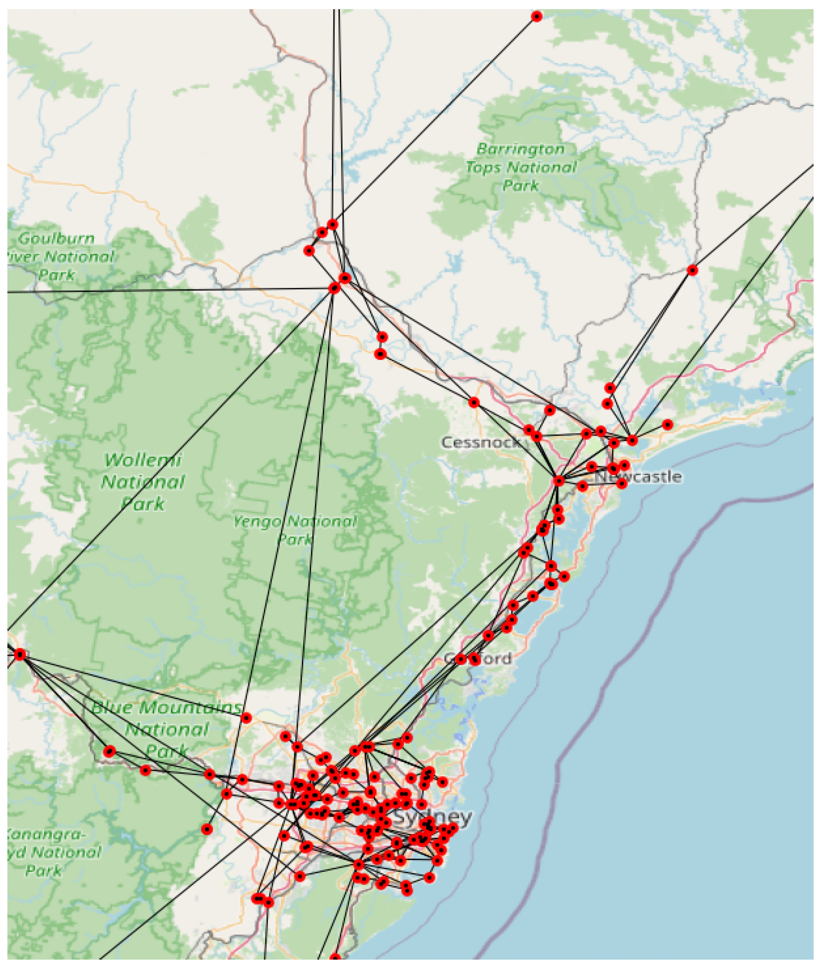
Publicly available distribution zone substation 15-min interval demand data from the Australian network operator Ausgrid [25] have been used for the machine learning-based node characterization in order to support computational reproducibility of this research. In particular, historic data from the year 2019 (between May 2018 and April 2019) and from the year 2020 (between May 2019 and April 2020) from 185 substations from distribution networks around Sydney and Newcastle have been used. These substations form the boundary between the sub-transmission network and the distribution (11 kV) network. The time is in Australian Eastern Standard Time (AEST) format during the winter period and Australian Eastern Daylight Time (AEDT) during the summer period. Figure 1 shows the irregular topology of the investigated distribution network, where real node positions (red dots) correspond to population density clusters, resulting in large variability of edge length (black lines).

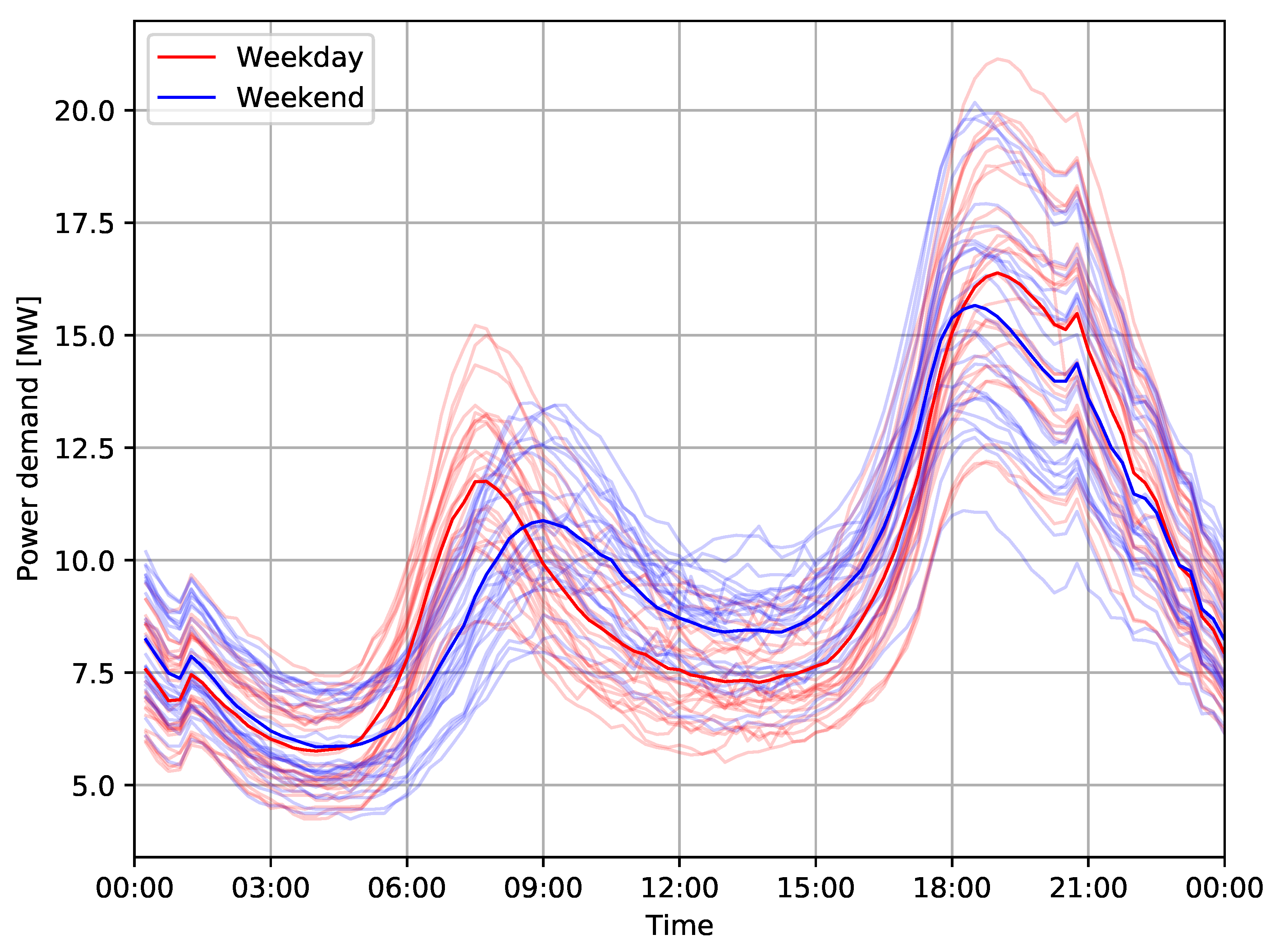
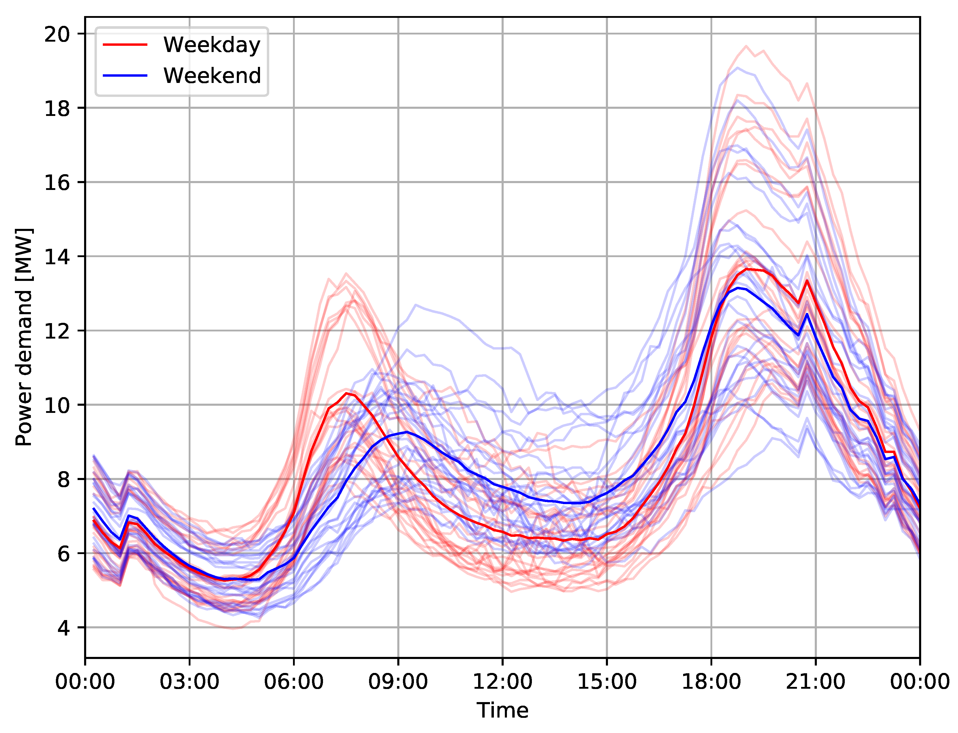
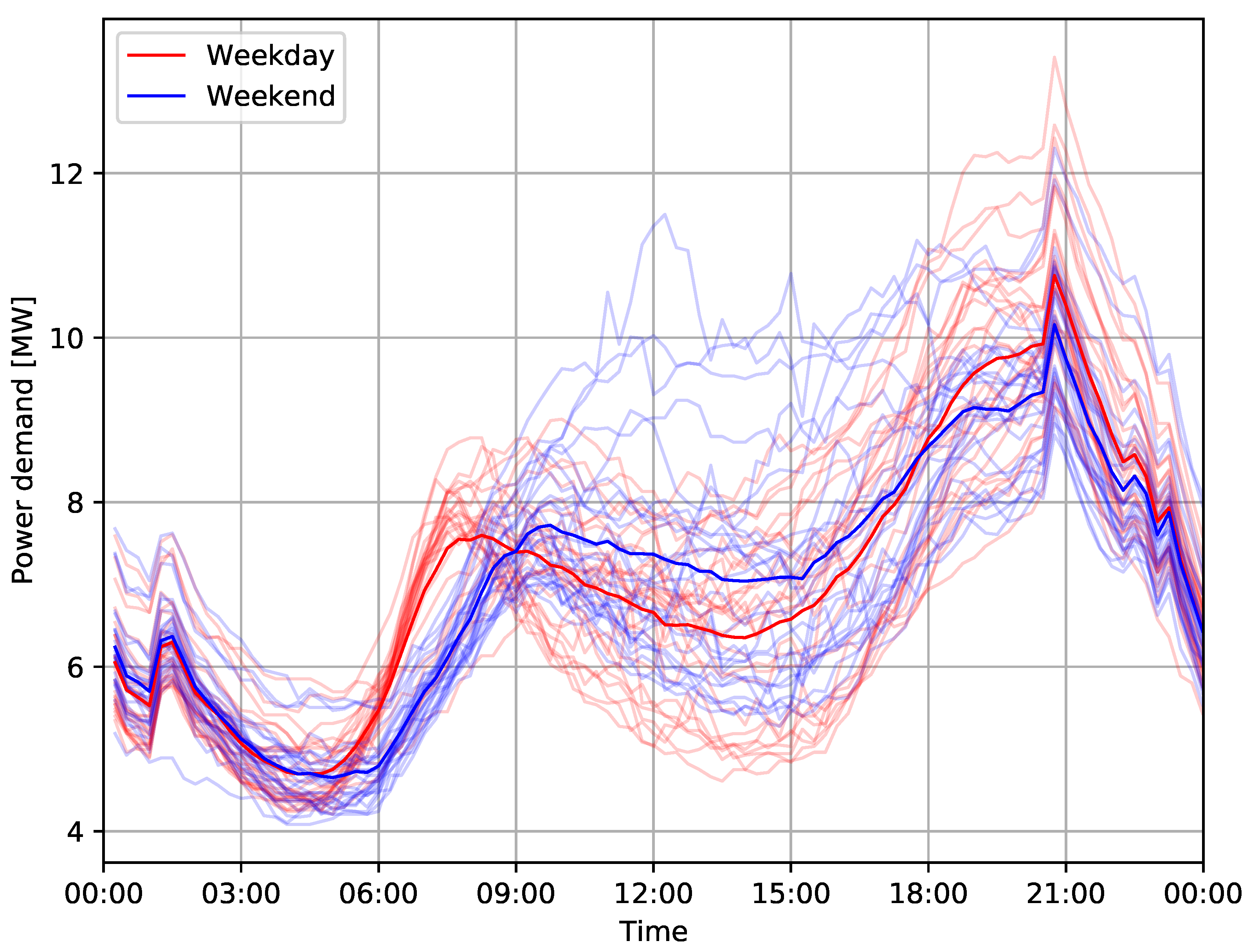
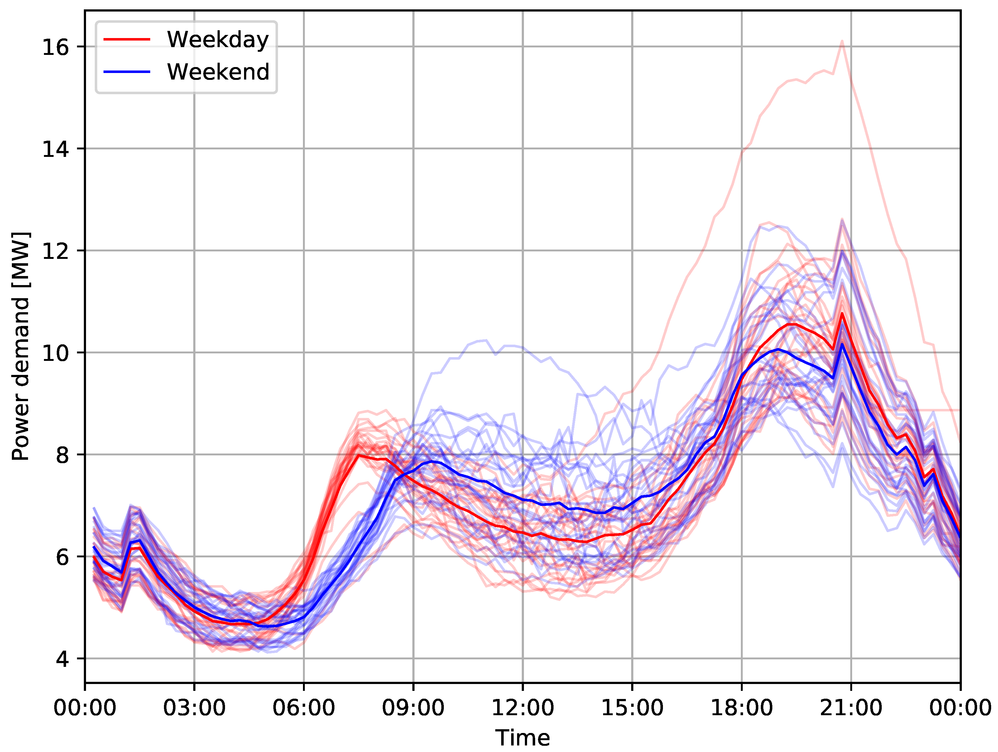
Data from individual substations were sampled at 15 min and divided into time series by days, resulting in 96 data points. The proposed classification cannot intentionally distinguish between workdays, weekends or holidays, as there is no information on the actual date attached to the individual time series, although the dataset exhibit typical daily, weekly and seasonal fluctuations in electricity demand. Nevertheless, the achieved accuracies are far from prohibitive, as discussed in the next chapter.

The daily fluctuations include morning and afternoon peaks throughout all four seasons, including workdays and weekends, see Figure 2, Figure 3, Figure 4 and Figure 5 for an example from Harbord substation, with group averages in dark color. In summer, a lower overall demand can be observed, including less distinct morning and evening peaks.

Clustering Analysis

In general, the goal of clustering is to identify structure in an unlabeled data set by objectively organizing data into homogeneous groups where the within-group-object similarity is minimized and the between-group-object dissimilarity is maximized [27]. The time-series demand data presented in this section have been clustered by the basic k-means algorithm [28] in order to split substations into several groups. K-means clustering is a renowned heuristic method for crisp partitions (i.e., each object belongs to exactly one cluster, as opposed to fuzzy if one object is allowed to be in more than one cluster to a different degree), where each cluster is represented by the mean value of the objects in the cluster.

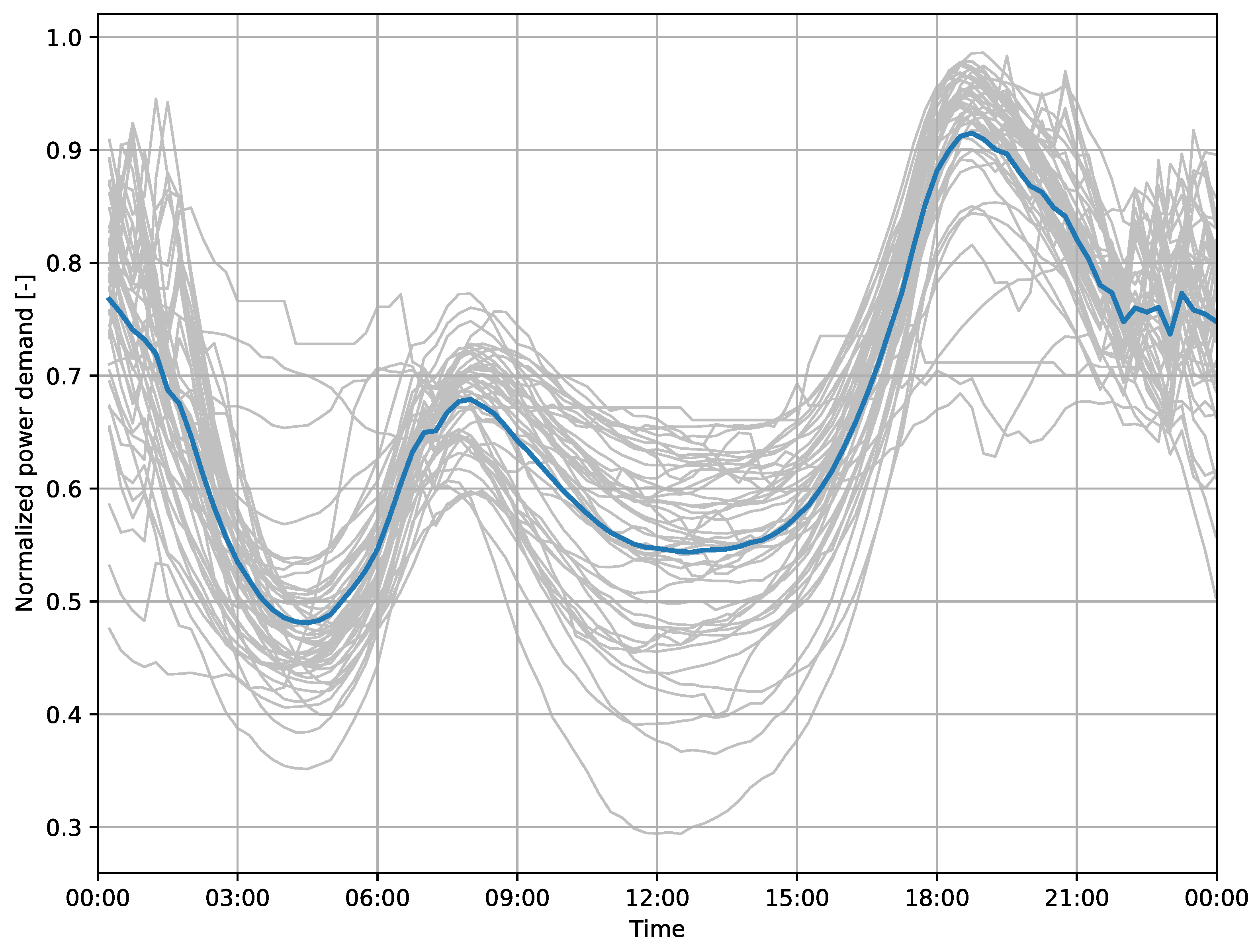
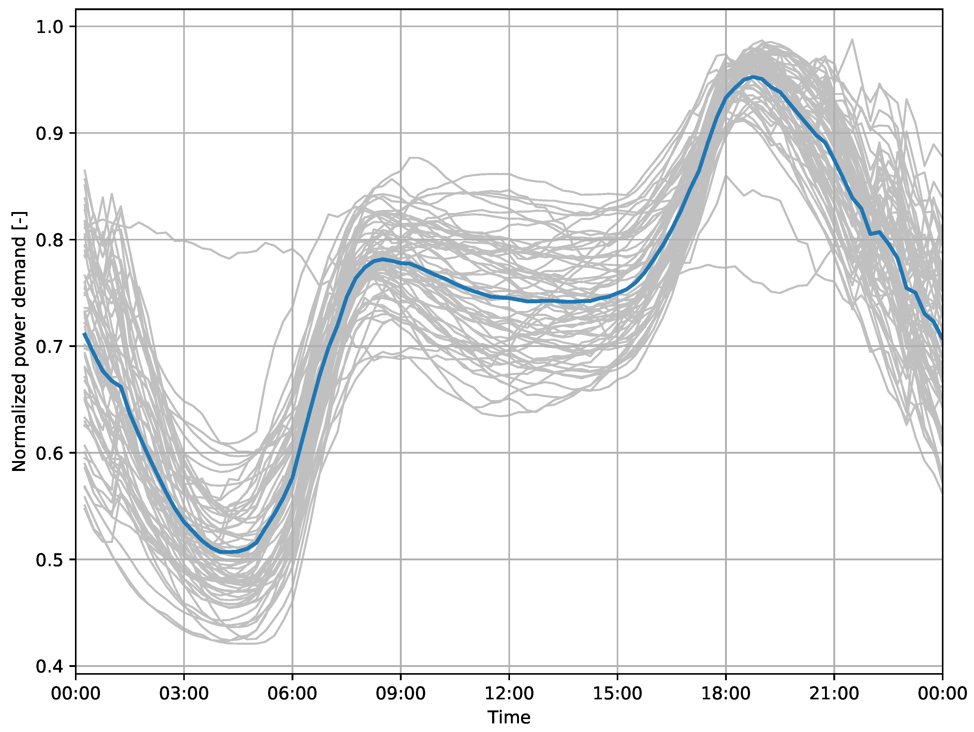
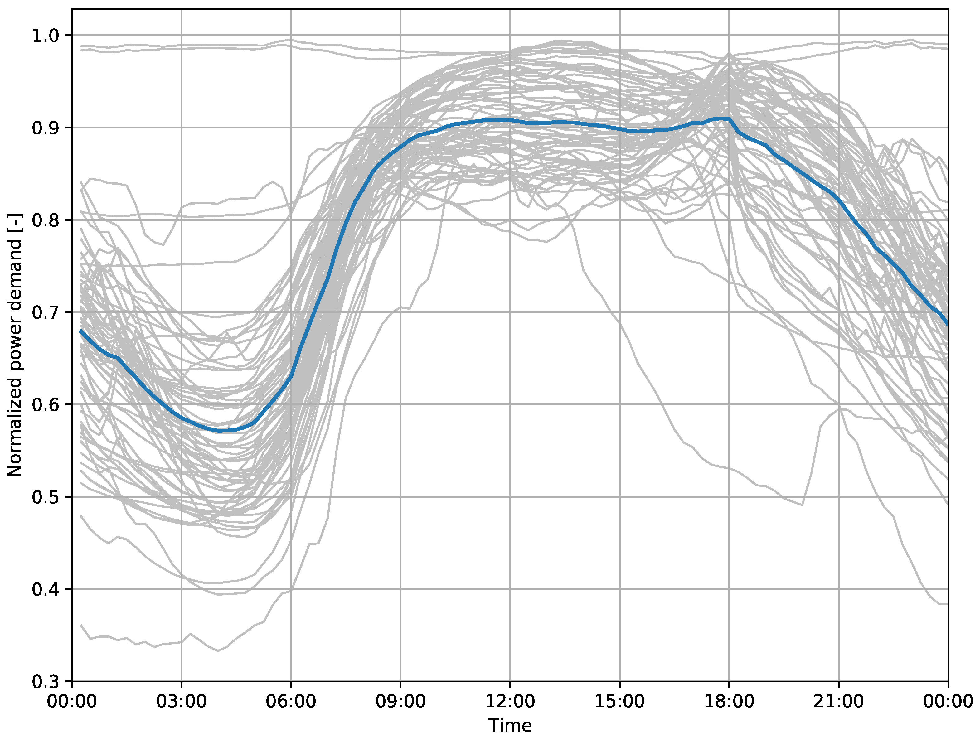
For effective optimization of the distribution grid, and for any network-level simulations in general, the behavior of nodes (i.e., stations and substations) must be understood. Daily fluctuations of power demand may depend on the type of supplied neighborhood. Three basic types of substation neighborhoods—residential, business and combined—were considered as only 96 equally spaced data points were available per signal. K-means clustering analysis with k = 3 identified the following clusters (Figure 6, Figure 7 and Figure 8):

• C1: 48 substations, residential, morning and evening demand peak,
• C2: 66 substations, combined, morning and evening peaks less distinct than in the clusters C1,
• C3: 71 substations, business, high and flat distribution of energy demand during the day.

Note that the qualitative evaluation of characteristics of the three identified clusters is based only on the assumption of daily peak distribution and has not been verified by any other on-site investigation as it was not the goal of this research. Note the normalization of amplitudes of daily signals to the maximum value in order to ensure classification based on demand patterns instead of absolute values of demand.

3. Machine Learning Based Classification

3.1. Surrogates Resampling

In each identified cluster, 14 substations have been randomly selected (see

Table 1. Selected substations for each cluster.

C1	C2	C3
Avondale	Baerami	Auburn
Cessnock South	Blakehurst	Blackwattle Bay
Edgeworth	Campsie	Brookvale
Harbord	Dulwich Hill	Camperdown
Jannali	Enfield	City East
Killarney	Gateshead	Darlinghurst
Medowie	Lindfield	Graving Dock
Mt Hutton	Maitland	Kotara
Newport	Nelson Bay	Lucas Heights
Paxton	Peats Ridge	New Lambton
Sans Souci	Riverwood	Newcastle CBD
Swansea	St Ives	Paddington
Tanilba Bay	Thornton	Surry Hills
Tomaree	Williamtown	Tomago

) for the machine learning-based classification. The goal is to identify a substation based on its daily demand, all selected substations being type 33/11 kV. Since data for all substations were not complete, a criterion for the minimal number of measurement days per substation has been set to 350 days of a year.

Three scenarios were evaluated considering data from year the 2019, 2020 and both years respectively. In the first two scenarios, data were divided between training and testing set using a typical split ratio 80%/20%. Data were selected randomly from the original dataset in such a way that the same split ratio is ensured for each substation. In order to avoid over-fitting and evaluate the reliability of the models, 10 splits of the dataset were randomly generated. This technique is often referred to as bootstrapping [29] and has been preferred over cross-validation due to the limited number of time series available, as cross-validation resamples without replacement and thus produces surrogate data sets that are smaller than the original. Bootstrapping used here resamples without replacement, produces surrogate datasets with the same number of time series as the original dataset, therefore statistical evaluation of the performance of the model becomes available, as represented here by the average confusion matrices and reported variability of accuracies. Each row in a confusion matrix represents the instances in a real class, while each column represents the instances in a predicted class, so whether the system is confusing two classes can easily be visible.

In the third scenario, denoted as 2019–2020, data from the year 2019 were used for training and data from the year 2020 for testing. Five runs for each cluster and model were done and their results averaged in order to consider variance due to random initialization of network parameters and data shuffling. This scenario aims to evaluate generalization capability of the used model for future years. Setup of all three scenarios is listed in

Table 2. Setup of the evaluated years and clusters.

Year	Cluster	No. of Classes	Dataset Size	Training Size	Testing Size	No. of Repeats
2019	C1	14	5085	4070	1015	10
	C2	14	5081	4068	1013	10
	C3	14	5085	4069	1016	10
2020	C1	14	5109	4091	1018	10
	C2	14	5098	4082	1016	10
	C3	14	5105	4087	1018	10
2019–2020	C1	14	10,194	5085	5109	5
	C2	14	10,179	5081	5098	5
	C3	14	10,190	5085	5105	5

.

3.2. CNN Models

Commonly used machine learning methods for the classification of time-series data are Support Vector Machines (SVM) and Artificial Neural Networks (ANN), as recently reported in [30,31,32].

SVM is a simple algorithm that looks for a hyperplane that divides the n-dimensional input space into two or more categories and assigns an output value accordingly. However, there is an infinite number of such planes, and the goal of the algorithm is to find a plane that has the maximum distance from the points of both (all) classes. Multidimensional problems are usually transformed using the so-called kernel transformation, so the non-linear problem is converted to linear. That means, from the original space to the Euclidean space. Thus, it is clear that the correct function of the SVM depends on the correct choice of the kernel function. This method is computationally expensive if large amounts of data are to be considered.

The best known and probably also the most universal ML algorithm is the Artificial Neural Network (ANN) method. This algorithm is inspired by the decision-making processes of the human brain. It is composed of several million neurons, which evaluate and pass information to each other. Likewise, an artificial neural network is composed of layers, which are composed of neurons. Each layer has given rules, based on which it evaluates the input information from the previous layer and passes the output to the next layer. Input and output can be of different formats. Within ANN, however, the information is transmitted using an internal weighing system. The number of layers and neurons in them is arbitrary, as well as the type of layers. However, all these parameters affect the reliability of ANN.

Both SVM and ANN are sensitive to the subjective choice of parameters, in the case of SVM, these are the describing (scalar) features of the time-series, such as the number of peaks, total energy or various Fourier transform properties. In the case of ANN, the subjective choice of its architecture can significantly influence both its performance as well as computational requirements. Given the relatively small size of the time series (96 data points), compared to applications that differ by two orders of magnitude, where high-frequency components have to be maintained, such as the dynamic response of railway track due to a passing train, which, if resampled to a lower resolution, looses its most important characteristics (see e.g., [30]), finding proper characterization for SVM input vector would make a little sense, since the entire time series vector can be directly processed by a more general ANN model.

Some advanced time series classification techniques can be used such as Least-Squares Wavelet (LSWAVE) [33]. The spectral and wavelet analyses are very useful for estimating trends and seasonal components of any time series and identifying their patterns in the time-frequency domain [34]. Herein, we directly classify the time series data and shall leave the use of wavelets to future research.

A specific type of ANN, the convolutional neural networks (CNN) were selected for data classification as they provide state-of-the-art performance for computer vision or time-series classification and are also widely adopted for end-to-end learning [35]. End-to-end approach utilizes raw time-series data without any preprocessing and manual feature extraction which often introduces unnecessary bias as extracted features are often domain-specific. Convolutional layers in CNN also enhance pattern recognition capabilities of the network.

In the following, three CNN models with different architectures have been considered:

• CNN1 has the same architecture as the best performing model CNN in [30]. It contains one convolutional layer with 64 filters followed by max-pooling layer, fully connected hidden layer and an output layer;
• CNN2 contains three convolutional layers with 128, 64 and 32 filters, respectively. Batch normalization and dropout with 25% probability is applied to the output of the last convolutional layer before passed to a max-pooling layer. The result of the pooling layer is flattened to one fully connected output layer. It is the deepest architecture with the largest number of layers with trainable parameters;
• CNN3 contains one convolutional layer with 64 filters followed by an average pooling layer with output size 20 and fully connected output layer. This architecture contains the lowest number of trainable parameters.

Rectified linear unit (ReLU) has been used between layers as an activation function for all presented architectures. Overview of parameters for evaluated architectures is presented in

Table 3. Number of layers and number of trainable parameters for the evaluated convolutional neural networks.

Model	CNN1	CNN2	CNN3
Number of layers with trainable parameters	4	6	3
Number of trainable parameters	123,498	122,830	18,446
Average training time (s) ${}^{1,2}$	96.4	99.5	93.6

¹ C2 dataset in year 2019 (4069 training samples), ² NVIDIA GeForce GTX 1050 Max-Q with 640 cores and 3 GB of memory.

.

Training has been executed in 20 epochs. Data were forwarded through the networks in batches of size 32. The learning rate has been set to 0.001, while Adam optimizer has been used to minimize cross-entropy loss function (which is a composition of negative log-likelihood and logarithmic softmax function).

A graphics processing unit (GPU) has been used for training, approximately 0.6–0.8 GB of memory has been required, and models with a lower number of parameters (CNN3) had only slightly lower training time.

4. Results

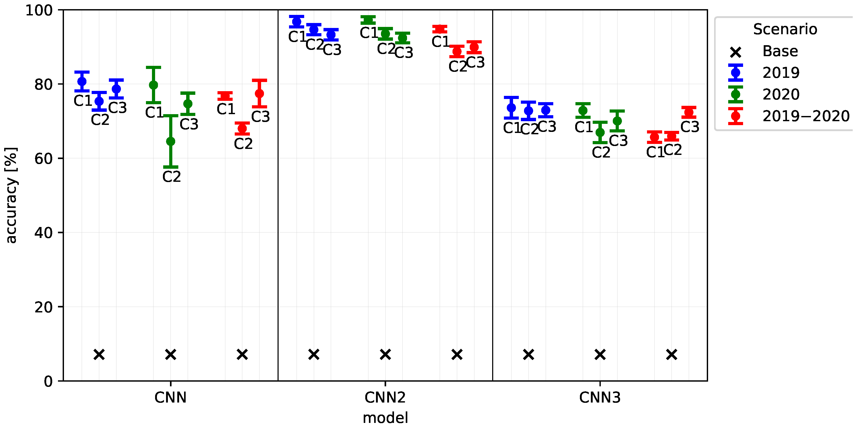
The most accurate model with mean accuracy over 88.8% and deviation less than 1.5% for all clusters and all scenarios is the CNN2 due to the incorporation of multiple convolutional layers. Slightly lower accuracy can be seen in the scenario 2019–2020, compared to the scenarios 2019 and 2020.

It was also shown that CNN2 model has the best ability to generalize future years (trained 2019, tested 2020), C1 cluster shows higher accuracy compared to C2 and C3.

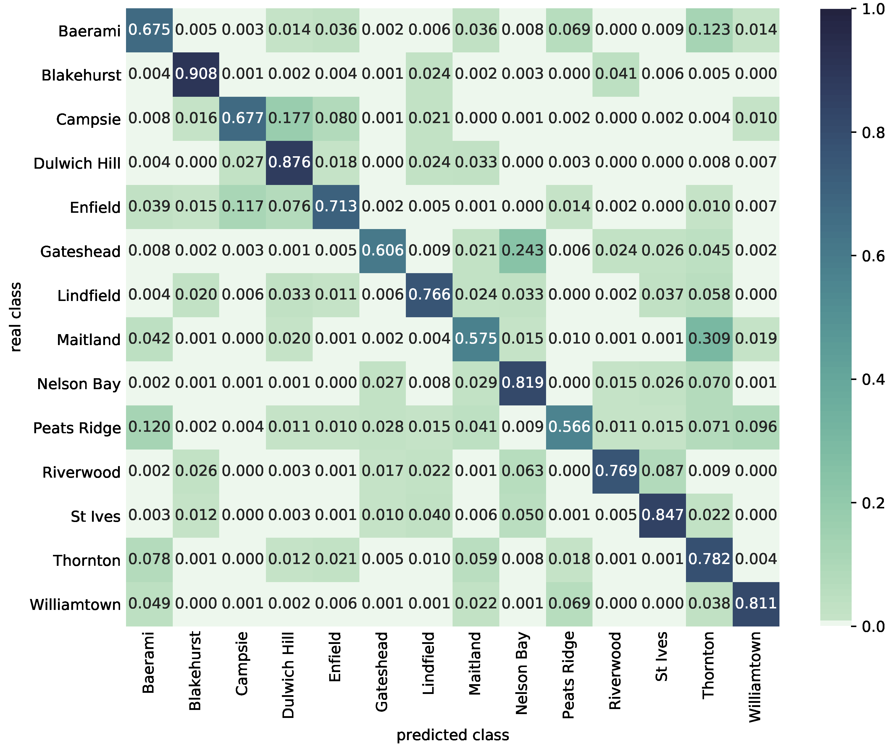
The highest mean accuracy can be observed in scenario 2019–2020 for CNN2 model and cluster C1 at Jannali substation (99.3%), while the lowest mean accuracy occurred in cluster C2 at Maitland substation (67.3%), which was often confused with Thornton.

The mean model accuracies are presented in

Table 4. Mean model accuracies for each year and cluster.

Year	Cluster	Base (%)	Mean (%)	CNN1 (%)	CNN2 (%)	CNN3 (%)
2019	C1	7.1	83.7 ± 10.0	80.7 ± 2.5	96.8 ± 1.4	73.6 ± 2.8
	C2	7.1	80.9 ± 10.0	75.3 ± 2.4	94.6 ± 1.4	72.8 ± 2.3
	C3	7.1	81.6 ± 8.8	78.7 ± 2.4	93.3 ± 1.4	72.9 ± 1.7
2020	C1	7.1	83.3 ± 10.7	79.7 ± 4.7	97.2 ± 0.9	72.9 ± 1.8
	C2	7.1	75.0 ± 13.8	64.5 ± 6.9	93.5 ± 1.4	66.9 ± 2.7
	C3	7.1	79.0 ± 9.9	74.7 ± 2.9	92.4 ± 1.3	70.0 ± 2.7
2019–2020	C1	7.1	79.1 ± 12.0	76.8 ± 0.9	94.8 ± 0.7	65.7 ± 1.4
	C2	7.1	74.2 ± 10.4	68.0 ± 1.5	88.8 ± 1.4	65.9 ± 1.0
	C3	7.1	79.9 ± 7.7	77.4 ± 3.6	89.9 ± 1.5	72.4 ± 1.3

or in graphical representation, Figure 9, where the accuracy of independent and random selection results (base) are also included for reference.

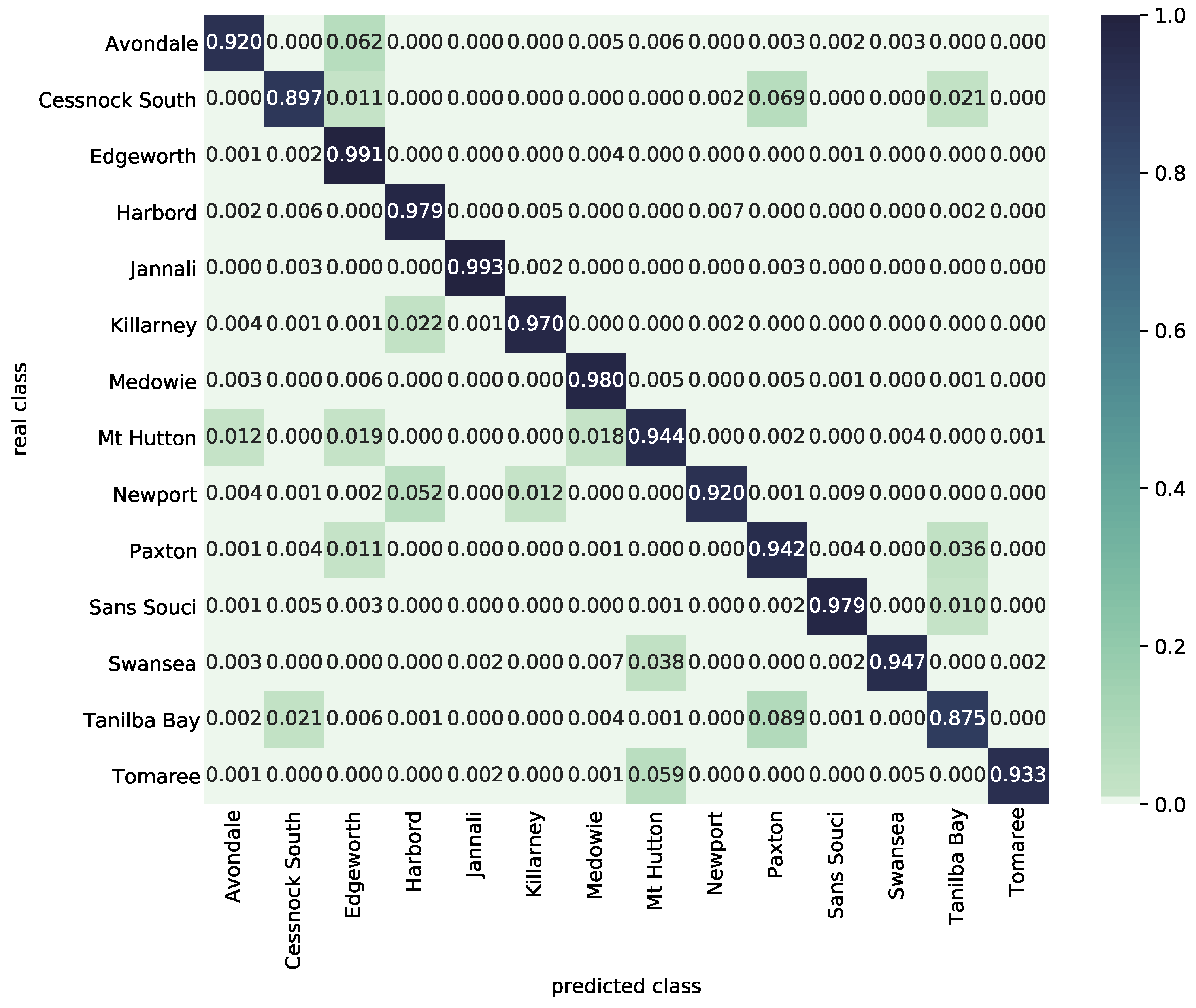
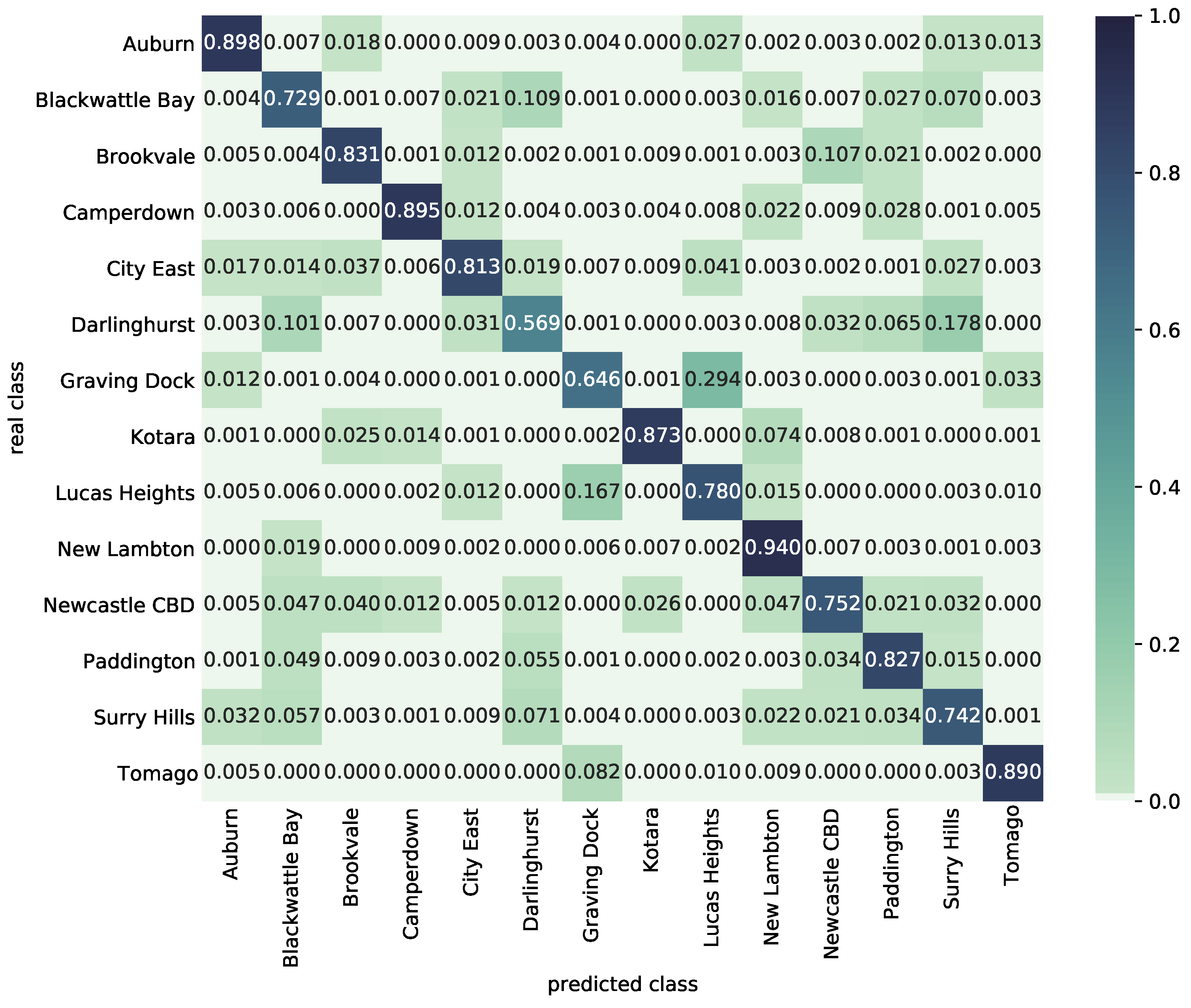
Results are presented by means of mean confusion matrices for scenario three (training on 2019 data and testing on 2020 data) and the best performing CNN2 classifier model for individual clusters C1 to C3, see Figure 10, Figure 11 and Figure 12. These matrices show how the model is able to cope with the classification of new data in future years and which classes (substations) are often confused.

5. Discussion

The machine learning-based substation node energy demand characterization represents a first logical step in a network-level flexibility assessment based on simulations or optimizations of DSM programs, ensuring resilient and stable operation of smart grids.

The resulting meta-models of individual substations can be further utilized to mitigate the difficulties associated with identifying, implementing and actuating various sources of energy flexibility, such as those related to the technology of indoor environmental comfort, compared to the few large ones traditionally acknowledged.

As explained and demonstrated in the paper, the ML-based classification of substations can be further utilized to study different scales of smart grid applications, and verify new control strategies. In particular, this study shows that:

(1)

Clustering analysis can effectively help to understand the type of supplied neighbourhood, such as residential, mixed or business, and is used in this paper for benchmarking categorization of the three convolutional neural network models.

(2)

Despite inherent daily (accounted timestamp), weekly (unaccounted directly) and seasonal (unaccounted directly) fluctuations in historic node demand data, the proposed CNN2 model yields relatively reliable results even when validated on future data, with mean model accuracy ranging from 88.8 + −1.4 (combined cluster C2) to 94.8 + −0.7 (residential cluster C1) in case of scenario 2019–2020.

(3)

Given the relatively high ratio of trainable parameters (e.g., 122,830 for CNN2) to the input size (96 data points), over-fitting and over-determinism can clearly represent a problem and has to be carefully acknowledged in general, however, due to the proposed state-of-the-art ANN architecture, including multiple convolutional layers accompanied with regularization techniques such as batch normalization and dropout and conservatively set learning rate, the presented sparse mean confusion matrices based on bootstrap (10× resampling) demonstrate a rather robust fit, if relatively small accuracy standard deviation of 1.4% (CNN2) and dominant diagonal are considered.

(4)

Certain classes may be mutually confused due to similarities in substations and their neighbourhoods. Some types of neighbourhood such as tourist or holiday locations may also increase demand variability in different parts of a year. The mutual confusions are similar for all investigated CNN models, and since these models have a different number of convolutional layers, the confusion is more likely to stem from substations variability rather than from the different architecture of CNN. For example, Swansea has fishing and tourism, Campsie has business and commercial areas, while Darlinghurst is a vibrant central district dependent on high season.

Limitations of this study include a limited range of considered years due to computational intensity. In order to optimize the distribution grid as a whole, network topology including its inner dependencies and boundary conditions must be considered (e.g., using hierarchical neural networks). In this study, only classification of network nodes was presented.

6. Conclusions

After introducing the importance of quantifying network flexibility potential for the safe integration of renewable energy sources and sustainable economy, the background on the smart grid and network modeling has been presented together with state-of-the-art machine learning techniques and their application to the classification of historical demand data. The resulting characterization of individual substations is important for future work on network-level simulations, the aim of which is to mitigate the difficulties associated with identifying, implementing and actuating many small sources of energy flexibility, compared to the few large ones traditionally acknowledged.

The proposed CNN models do not require any pre-processing of the 15 min interval demand data, the only subjective choice associated with the classification is the architecture of the neural network. Three scenarios were evaluated considering data from year 2019, 2020 and both years respectively. In the first two scenarios, data were divided between training and testing set using a typical split ratio 80/20, and in the third scenario, denoted as 2019–2020, data from the year 2019 were used for training and data from the year 2020 for testing. This enabled the verification of both statistical significance of the classifier, based on bootstrapping, as well as generalization of the resulting meta-models.

The sparse mean confusion matrices indicate a robust modeling approach, considering very similar structures across the investigated architectures, and relatively small standard deviation of accuracies. A more detailed (qualitative) assessment of substations and their neighbourhoods was beyond the scope of this paper, as well as the effects of boundary conditions on real network topology. Future work will continue with hierarchical neural networks modeling of the entire network.