
Does Air Pollution Decrease Labor Supply of the Rural Middle-Aged and Elderly?


Abstract
:1. Introduction
2. Data
2.1. Data
2.2. Variables
2.2.1. Dependent Variable
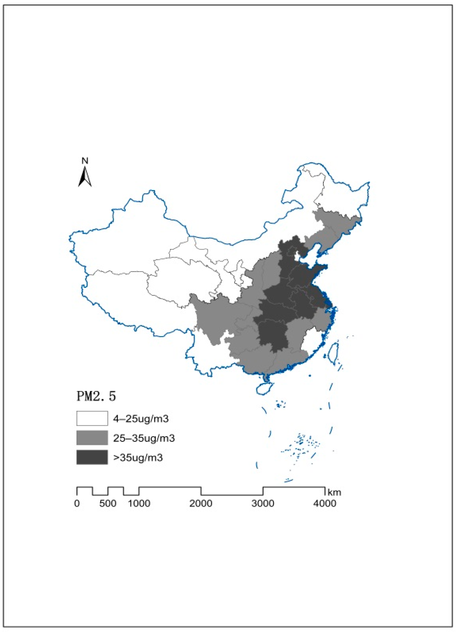
2.2.2. Independent Variables: PM2.5
2.2.3. Other Control Variables
2.3. Descriptive Statistics
3. Regression Analysis
3.1. Multiple Linear Regression
3.2. Heckman Selection Model
3.3. Binary Probit Model
4. Results
4.1. Effects of PM2.5 on Working Hours
4.2. Heterogeneous Effects of PM2.5 on Working Hours
4.2.1. Heterogeneous Effects of PM2.5 on Working Hours by Income
4.2.2. Heterogeneous Effects of PM2.5 on Working Hours by Geographical Regions
4.3. Mechanisms That Link between PM2.5 and Working Hours
4.4. Robustness Check
4.4.1. Robustness Check 1: Fixed-Effect Estimation
4.4.2. Robustness Check 2: Estimation of AQI and Six Air Pollutants on Working Hours
5. Conclusions and Policy Implications
Author Contributions
Funding
Institutional Review Board Statement
Informed Consent Statement
Data Availability Statement
Conflicts of Interest
References
- Li, B.; Wu, X. Economic Structure and Intensity Influence Air Pollution Model. Energy Procedia 2011, 5. [Google Scholar] [CrossRef] [Green Version]
- Yi, F.; Ye, H.; Wu, X.; Zhang, Y.Y.; Jiang, F. Self-Aggravation Effect of Air Pollution: Evidence from Residential Electricity Consumption in China. Energy Econ. 2020, 86. [Google Scholar] [CrossRef]
- Dockery, D. Acute Respiratory Effects of Particulate Air Pollution. Annu. Rev. Public Health 1994, 15. [Google Scholar] [CrossRef]
- Pope, C.A. Epidemiology of Fine Particulate Air Pollution and Human Health: Biologic Mechanisms and Who’s at Risk? Environ. Health Perspect. 2000, 108 (Suppl. 4). [Google Scholar] [CrossRef] [Green Version]
- Seaton, A.; Godden, D.; MacNee, W.; Donaldson, K. Particulate Air Pollution and Acute Health Effects. Lancet 1995, 345. [Google Scholar] [CrossRef]
- Pope, C.A.; Dockery, D.W. Air Pollution and Life Expectancy in China and Beyond. Proc. Natl. Acad. Sci. USA 2013, 110, 12861–12862. [Google Scholar] [CrossRef] [Green Version]
- Zivin, J.G.; Neidell, M. The Impact of Pollution on Worker Productivity. Am. Econ. Rev. 2012, 102. [Google Scholar] [CrossRef] [Green Version]
- Zhang, Y.Y.; Zheng, Q.; Wang, H. Challenges and Opportunities Facing the Chinese Economy in the New Decade: Epidemics, Food, Labor, E-Commerce, and Trade. Chin. Econ. 2021, 1–3. [Google Scholar] [CrossRef]
- Breneman, D.W.; Schultz, T.W. Investing in People: The Economics of Population Quality. J. Policy Anal. Manag. 1982, 1. [Google Scholar] [CrossRef]
- Berkowitz, M.; Johnson, W.G. Health and Labor Force Participation. J. Hum. Resour. 1974, 9. [Google Scholar] [CrossRef]
- Dwyer, D.S.; Mitchell, O.S. Health Problems as Determinants of Retirement: Are Self-Rated Measures Endogenous? J. Health Econ. 1999, 18. [Google Scholar] [CrossRef] [Green Version]
- Trevisan, E.; Zantomio, F. The Impact of Acute Health Shocks on the Labour Supply of Older Workers: Evidence from Sixteen European Countries. Labour Econ. 2016, 43. [Google Scholar] [CrossRef] [Green Version]
- Kalwij, A.; Vermeulen, F. Health and Labour Force Participation of Older People in Europe: What Do Ojective Health Indicators Add to the Analysis? Health Econ. 2008, 17. [Google Scholar] [CrossRef]
- Li, Q.; Lei, X.; Zhao, Y. The Effect of Health on the Labor Supply of Middle-aged and Older Chinese. China Econ. Q. 2014, 13, 917–938. [Google Scholar]
- Ning, M.; Gong, J.; Zheng, X.; Zhuang, J. Does New Rural Pension Scheme Decrease Elderly Labor Supply? Evidence from CHARLS. China Econ. Rev. 2016, 41, 315–330. [Google Scholar] [CrossRef]
- Aragón, F.M.; Miranda, J.J.; Oliva, P. Particulate Matter and Labor Supply: The Role of Caregiving and Non-Linearities. J. Environ. Econ. Manag. 2017, 86. [Google Scholar] [CrossRef] [Green Version]
- Hanna, R.; Oliva, P. The Effect of Pollution on Labor Supply: Evidence from a Natural Experiment in Mexico City. J. Public Econ. 2015, 122. [Google Scholar] [CrossRef] [Green Version]
- Yamada, D.; Narita, D. The Effects of Air Pollution on Labor Supply in Japan: A Panel Data Analysis Based on PM2.5 Pollution and Labor Data. SSRN Electron. J. 2020. [Google Scholar] [CrossRef]
- Qin, B. Research on Industrial Pollution in Rural China: Seeking a Solution to the Pollution Incurred to the Farmers. In Sustainable Development in Rural China; Springer: Berlin/Heidelberg, Germany, 2015. [Google Scholar] [CrossRef]
- Aunan, K.; Hansen, M.H.; Liu, Z.; Wang, S. The Hidden Hazard of Household Air Pollution in Rural China. Environ. Sci. Policy 2019, 93. [Google Scholar] [CrossRef]
- Balmes, J.R. Household Air Pollution from Domestic Combustion of Solid Fuels and Health. J. Allergy Clin. Immunol. 2019. [Google Scholar] [CrossRef]
- Lin, B.; Lin, Z.; Zhang, Y.Y.; Liu, W. The Impact of the New Rural Pension Scheme on Retirement Sustainability in China: Evidence of Regional Differences in Formal and Informal Labor Supply. Sustainability 2018, 10, 4366. [Google Scholar] [CrossRef] [Green Version]
- Lin, B.; Zhang, Y.Y. The Impact of Fiscal Subsidies on the Sustainability of China’s Rural Pension Program. Sustainability 2020, 12, 186. [Google Scholar] [CrossRef] [Green Version]
- Jin Feng, Y.Y. Income Inequality and Health in Rural China. Econ. Res. J. 2007, 1, 26–35. (In Chinese) [Google Scholar]
- Chang, T.; Zivin, J.G.; Gross, T.; Neidell, M. Particulate Pollution and the Productivity of Pear Packers. Am. Econ. J. Econ. Policy 2016, 8. [Google Scholar] [CrossRef] [Green Version]
- He, J.; Liu, H.; Salvo, A. Severe Air Pollution and Labor Productivity: Evidence from Industrial Towns in China. Am. Econ. J. Appl. Econ. 2019, 11. [Google Scholar] [CrossRef] [Green Version]
- Li, T.; Liu, H.; Salvo, A. Severe Air Pollution and Labor Productivity: Evidence from Industrial Towns in China. SSRN Electron. J. 2015. [Google Scholar] [CrossRef] [Green Version]
- Archsmith, J.; Heyes, A.; Saberian, S. Air Quality and Error Quantity: Pollution and Performance in a High-Skilled, Quality-Focused Occupation. J. Assoc. Environ. Resour. Econ. 2018, 5. [Google Scholar] [CrossRef]
- Liu, J.; Rozelle, S.; Xu, Q.; Yu, N.; Zhou, T. Social Engagement and Elderly Health in China: Evidence from the China Health and Retirement Longitudinal Survey (CHARLS). Int. J. Environ. Res. Public Health 2019, 16, 278. [Google Scholar] [CrossRef] [Green Version]
- Lei, X.; Sun, X.; Strauss, J.; Zhao, Y.; Yang, G.; Hu, P.; Hu, Y.; Yin, X. Reprint of: Health Outcomes and Socio-Economic Status among the Mid-Aged and Elderly in China: Evidence from the CHARLS National Baseline Data. J. Econ. Ageing 2014, 4, 59–73. [Google Scholar] [CrossRef]
- Beatty, T.K.M.; Shimshack, J.P. School Buses, Diesel Emissions, and Respiratory Health. J. Health Econ. 2011, 30. [Google Scholar] [CrossRef]
- Arden Pope, C. Respiratory Disease Associated with Community Air Pollution and a Steel Mill, Utah Valley. Am. J. Public Health 1989, 79. [Google Scholar] [CrossRef] [Green Version]
- Pi, T.; Wu, H.; Li, X. Does Air Pollution Affect Health and Medical Insurance Cost in the Elderly: An Empirical Evidence from China. Sustainability 2019, 11, 1526. [Google Scholar] [CrossRef] [Green Version]
- Yu, G.; Wang, F.; Hu, J.; Liao, Y.; Liu, X. Value Assessment of Health Losses Caused by PM2.5 in Changsha City, China. Int. J. Environ. Res. Public Health 2019, 16, 2063. [Google Scholar]
- Benjamin, E.J.; Virani, S.S.; Callaway, C.W.; Chamberlain, A.M.; Chang, A.R.; Cheng, S.; Chiuve, S.E.; Cushman, M.; Delling, F.N.; Deo, R.; et al. Heart Disease and Stroke Statistics-2018 Update: A Report from the American Heart Association. Circulation 2018, 137. [Google Scholar] [CrossRef]
- Wooldridge, J.M. What’s New in Econometrics? Available online: https://scholar.harvard.edu/imbens/classes/nber-course-whats-new-econometrics (accessed on 1 March 2007).
- Zhu, L.; Hao, Y.; Lu, Z.N.; Wu, H.; Ran, Q. Do Economic Activities Cause Air Pollution? Evidence from China’s Major Cities. Sustain. Cities Soc. 2019, 49. [Google Scholar] [CrossRef]
- Zhang, Y.J.; Jin, Y.L.; Zhu, T.T. The Health Effects of Individual Characteristics and Environmental Factors in China: Evidence from the Hierarchical Linear Model. J. Clean. Prod. 2018, 194, 554–563. [Google Scholar] [CrossRef]
- Heckman, J. Sample Selection Bias as a Specification Error. Econometrica 1979, 47, 153–161. [Google Scholar]
- Wooldridge, J.M. Introductory Econometrics: A Modern Approach; Cengage Learning: Stanford, CA, USA, 2013. [Google Scholar]
- Puhani, P.A. The Heckman Correction for Sample Selection and Its Critique. J. Econ. Surv. 2000, 14. [Google Scholar] [CrossRef]
- Diamanti, S.; Longoni, M.; Agostoni, E.C. Leading Symptoms in Cerebrovascular Diseases: What about Headache? Neurol. Sci. 2019. [Google Scholar] [CrossRef]
- Zhang, Z.; Hao, Y.; Lu, Z.N. Does Environmental Pollution Affect Labor Supply? An Empirical Analysis Based on 112 Cities in China. J. Clean. Prod. 2018, 190. [Google Scholar] [CrossRef]
- Lu, M.; Wang, E. Forging Ahead and Falling behind: Changing Regional Inequalities in Post-Reform China. Growth Chang. 2002, 33. [Google Scholar] [CrossRef]
- Zheng, J.; Jiang, P.; Qiao, W.; Zhu, Y.; Kennedy, E. Analysis of Air Pollution Reduction and Climate Change Mitigation in the Industry Sector of Yangtze River Delta in China. J. Clean. Prod. 2016, 114. [Google Scholar] [CrossRef]
- Baltagi, B.H.; Sun, Y.; Zhang, Y.Y.; Li, Q. Nonparametric Panel Data Regression Models. In The Oxford Handbook of Panel Data; Baltagi, B.H., Ed.; Oxford University Press: Oxford, UK, 2015. [Google Scholar] [CrossRef]
- Zhang, Y.Y.; Gu, J.; Li, Q. Nonparametric Panel Estimation of Online Auction Price Processes. Empir. Econ. 2011, 40. [Google Scholar] [CrossRef] [Green Version]

| Variables | Definition | Mean | Std. dev |
|---|---|---|---|
| Work hour | Total working time in the past year (hours) | 1461.186 | 1112.22 |
| Chronic_disease | Have been diagnosed with chronic respiratory diseases or cardio-cerebrovascular diseases in the past two years, yes = 1, otherwise = 0 | 0.110 | 0.313 |
| PM2.5 | The mean PM2.5 concentration of the current and lag one year | 39.099 | 16.381 |
| Age | Age | 59.589 | 9.217 |
| Job | Engaged in agriculture = 1; otherwise = 0 | 0.752 | 0.432 |
| Edu | Years of receiving education | 4.040 | 3.374 |
| Sex | Male = 1, female = 0 | 0.484 | 0.500 |
| Other_chronic | Have been diagnosed with other chronic diseases in the past two years, yes = 1,otherwise = 0 | 0.111 | 0.314 |
| Marital_status | Married, cohabitating = 1, otherwise = 0 | 0.884 | 0.320 |
| Childhood_health | The health condition during childhood, excellent = 4, very good = 3, good = 2, fair = 1, poor = 0 | 2.211 | 1.105 |
| Ave_income | The per capita household income of last year (thousand) | 5.637 | 14.142 |
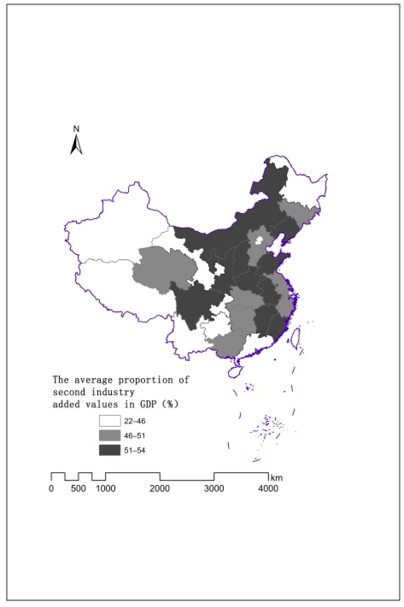
| Second_industry | The average proportion of secondary industry added value in GDP (%) | 49.059 | 7.508 |
| Dum_2013 | Dum_2013 = 1, reference: year = 2011 | 0.351 | 0.477 |
| Dum_2015 | Dum_2015 = 1, reference: year = 2011 | 0.359 | 0.480 |
| Dum_Central | Central region = 1,reference: east region | 0.301 | 0.459 |
| Dum_West | West region = 1, reference: east region | 0.261 | 0.439 |
| Dum_Northeast | Northeast region = 1, reference: east region | 0.089 | 0.284 |
| [1] OLS Whole Sample | [2] OLS Sample of Worked Individuals | [3] Heckman Selection Model | ||||
|---|---|---|---|---|---|---|
| Coef | Se | Coef | Se | Coef | Se | |
| Log_PM2.5 | −0.0362 * | (0.0204) | −0.0375 *** | (0.0123) | −0.0359 *** | (0.0124) |
| Age | −0.0126 *** | (0.0012) | −0.0026 *** | (0.0007) | −0.0009 | (0.0010) |
| Job | −0.7458 *** | (0.0204) | −0.3602 *** | (0.0121) | −0.2818 *** | (0.0356) |
| Edu | −0.0167 *** | (0.0029) | 0.0000 | (0.0017) | 0.0008 | (0.0018) |
| Sex | 0.2300 *** | (0.0189) | 0.0540 *** | (0.0115) | 0.0316 ** | (0.0150) |
| Other_chronic | −0.0506 * | (0.0277) | −0.0212 | (0.0169) | −0.0166 | (0.0171) |
| Marital_status | 0.1931 *** | (0.0323) | 0.0564 *** | (0.0202) | 0.0108 | (0.0282) |
| Childhood_health | 0.0027 | (0.0079) | 0.0047 | (0.0048) | 0.0076 | (0.0050) |
| Ave_income | −0.0031 | (0.0052) | 0.0103 *** | (0.0032) | 0.0117 *** | (0.0033) |
| Second_industry | −0.0132 *** | (0.0012) | −0.0054 *** | (0.0007) | −0.0046 *** | (0.0008) |
| Dum_2013 | −0.0751 *** | (0.0216) | −0.0332 ** | (0.0129) | −0.0328 ** | (0.0129) |
| Dum_2015 | −0.2824 *** | (0.0216) | −0.0880 *** | (0.0130) | −0.0873 *** | (0.0130) |
| Dum_Central | −0.0970 *** | (0.0216) | −0.1108 *** | (0.0132) | −0.1098 *** | (0.0132) |
| Dum_West | 0.1547 *** | (0.0243) | 0.0327 ** | (0.0146) | 0.0348 ** | (0.0146) |
| Dum_Northeast | −0.0805 ** | (0.0352) | −0.1229 *** | (0.0213) | −0.1227 *** | (0.0213) |
| Constant | 8.7417 *** | (0.1189) | 8.0709 *** | (0.0717) | 8.0060 *** | (0.0771) |
| select | ||||||
| Log_PM2.5 | −0.0044 | (0.0194) | ||||
| Job | −1.1831 *** | (0.0296) | ||||
| Edu | −0.0143 *** | (0.0032) | ||||
| Sex | 0.3045 *** | (0.0210) | ||||
| Other_chronic | −0.0538 * | (0.0299) | ||||
| Marital_status | 0.5130 *** | (0.0298) | ||||
| Childhood_health | −0.0388 *** | (0.0087) | ||||
| Ave_income | −0.0200 *** | (0.0055) | ||||
| Second_industry | −0.0096 *** | (0.0013) | ||||
| Retire | −0.4259 *** | −0.021 | ||||
| Constant | 1.5996 *** | (0.0945) | ||||
| mills | −0.1667 ** | (0.0711) | ||||
| R-squared | 0.1305 | 0.1033 | ||||
| Observations | 17,025 | 13,715 | 20,972 | |||
| Low-Income | Middle-Income | High-Income | ||||
|---|---|---|---|---|---|---|
| (<3000 CNY) | (3000–8800 CNY) | (>8800 CNY) | ||||
| Coef | Se | Coef | Se | Coef | Se | |
| Log_PM2.5 | −0.0295 * | 0.0171 | −0.0466 * | 0.0274 | −0.0267 | 0.024 |
| Age | −0.0030 ** | 0.0015 | 0.0019 | 0.0021 | 0.0009 | 0.002 |
| Job | −0.2164 *** | 0.0378 | −0.2294 *** | 0.0884 | −0.3577 *** | 0.1063 |
| Edu | 0.0009 | 0.0025 | 0.0008 | 0.0039 | 0.0007 | 0.0033 |
| Sex | 0.0423 ** | 0.0207 | 0.0118 | 0.0335 | 0.0232 | 0.0278 |
| Other_chronic | −0.0305 | 0.0243 | 0.0442 | 0.0365 | −0.0435 | 0.0326 |
| Marital_status | 0.032 | 0.0409 | −0.0429 | 0.0634 | 0.0541 | 0.0469 |
| Childhood_health | 0.0082 | 0.0069 | 0.0046 | 0.011 | 0.0077 | 0.0096 |
| Second_industry | −0.0060 *** | 0.0011 | −0.0048 *** | 0.0018 | −0.0023 | 0.0015 |
| Dum_2013 | −0.0601 *** | 0.018 | −0.0095 | 0.0259 | −0.0262 | 0.0253 |
| Dum_2015 | −0.0872 *** | 0.0177 | −0.1069 *** | 0.0288 | −0.1136 *** | 0.0257 |
| Dum_Central | −0.0997 *** | 0.0186 | −0.1003 *** | 0.0279 | −0.1125 *** | 0.0253 |
| Dum_West | 0.0468 ** | 0.0204 | 0.0329 | 0.0309 | 0.0379 | 0.0288 |
| Dum_Northeast | −0.1236 *** | 0.0293 | −0.1335 *** | 0.0455 | −0.0322 | 0.043 |
| Constant | 8.0159 *** | 0.1028 | 7.9529 *** | 0.1742 | 7.8191 *** | 0.1584 |
| select | ||||||
| Log_PM2.5 | 0.0086 | 0.0246 | −0.0266 | 0.043 | −0.0366 | 0.0477 |
| Job | −0.8420 *** | 0.0421 | −1.2770 *** | 0.0625 | −1.6296 *** | 0.0589 |
| Edu | −0.0119 *** | 0.0042 | −0.0157 ** | 0.0071 | −0.0158 ** | 0.0075 |
| Sex | 0.2866 *** | 0.0265 | 0.3109 *** | 0.0476 | 0.3091 *** | 0.0515 |
| Other_chronic | −0.0960 ** | 0.0386 | −0.0395 | 0.0649 | 0.0672 | 0.071 |
| Marital_status | 0.5539 *** | 0.0367 | 0.5260 *** | 0.0688 | 0.3670 *** | 0.0784 |
| Childhood_health | −0.0470 *** | 0.0109 | −0.0464 ** | 0.0197 | −0.0097 | 0.0211 |
| Second_industry | −0.0102 *** | 0.0017 | −0.0129 *** | 0.0029 | −0.0043 | 0.0032 |
| Retire | −0.4707 *** | 0.0265 | −0.3432 *** | 0.0467 | −0.3643 *** | 0.0526 |
| Constant | 1.3216 *** | 0.12 | 1.9604 *** | 0.2088 | 1.7725 *** | 0.2342 |
| mills | −0.0706 | 0.0915 | −0.3320 * | 0.1755 | −0.2571 | 0.1626 |
| Observations | 12,051 | 4444 | 4477 | |||
| East | Central | West | Northeast | |||||
|---|---|---|---|---|---|---|---|---|
| Coef | Se | Coef | Se | Coef | Se | Coef | Se | |
| Log_PM2.5 | −0.0158 | 0.0200 | −0.1849 *** | 0.0369 | 0.0042 | 0.0258 | −0.1196 *** | 0.0303 |
| Age | −0.0032 * | 0.0017 | −0.0006 | 0.0018 | −0.0010 | 0.0020 | −0.0010 | 0.0041 |
| Job | −0.2947 *** | 0.0642 | −0.3529 *** | 0.0660 | −0.1335 ** | 0.0646 | −0.3590 *** | 0.0688 |
| Edu | 0.0046 | 0.0029 | −0.0035 | 0.0032 | 0.0007 | 0.0040 | 0.0041 | 0.0061 |
| Sex | 0.0421 * | 0.0240 | 0.0300 | 0.0309 | 0.0112 | 0.0263 | 0.0335 | 0.0412 |
| Other_chronic | 0.0027 | 0.0308 | −0.0617 ** | 0.0313 | −0.0043 | 0.0314 | −0.0271 | 0.0558 |
| Marital_status | −0.0113 | 0.0419 | −0.0016 | 0.0525 | 0.0169 | 0.0682 | 0.0533 | 0.1028 |
| Childhood_health | 0.0015 | 0.0080 | 0.0106 | 0.0089 | 0.0144 | 0.0110 | 0.0198 | 0.0166 |
| Ave_income | 0.0202 *** | 0.0054 | 0.0045 | 0.0062 | 0.0085 | 0.0060 | 0.0225 * | 0.0129 |
| Second_industry | −0.0021 | 0.0017 | −0.0084 *** | 0.0016 | −0.0031 ** | 0.0013 | −0.0010 | 0.0042 |
| Dum_2013 | −0.0283 | 0.0216 | −0.0385 | 0.0237 | −0.0158 | 0.0249 | −0.0725 * | 0.0430 |
| Dum_2015 | −0.0673 *** | 0.0223 | −0.0688 *** | 0.0241 | −0.1206 *** | 0.0248 | −0.0588 | 0.0485 |
| Constant | 7.9337 *** | 0.1352 | 8.7242 *** | 0.1931 | 7.7255 *** | 0.1205 | 7.9426 *** | 0.2745 |
| select | ||||||||
| Log_PM2.5 | 0.1154 *** | 0.0364 | −0.0391 | 0.0641 | −0.0387 | 0.0476 | 0.1616 *** | 0.0466 |
| Job | −1.3623 *** | 0.0463 | −1.2120 *** | 0.0550 | −0.9187 *** | 0.0654 | −1.0076 *** | 0.1075 |
| Edu | −0.0013 | 0.0056 | −0.0152 *** | 0.0058 | −0.0281 *** | 0.0067 | 0.0041 | 0.0113 |
| Sex | 0.3142 *** | 0.0371 | 0.3693 *** | 0.0384 | 0.2021 *** | 0.0403 | 0.2799 *** | 0.0688 |
| Other_chronic | −0.0886 | 0.0542 | −0.0532 | 0.0550 | −0.0260 | 0.0571 | −0.0852 | 0.0934 |
| Marital_status | 0.4735 *** | 0.0522 | 0.4972 *** | 0.0556 | 0.6046 *** | 0.0531 | 0.5830 *** | 0.1316 |
| Childhood_health | −0.0008 | 0.0151 | 0.0056 | 0.0158 | −0.0741 *** | 0.0175 | −0.0546 * | 0.0299 |
| Ave_income | −0.0105 | 0.0093 | −0.0293 *** | 0.0102 | −0.0034 | 0.0108 | 0.0083 | 0.0225 |
| Second_industry | −0.0097 *** | 0.0031 | −0.0178 *** | 0.0021 | −0.0041 * | 0.0023 | 0.0226 *** | 0.0063 |
| Retire | −0.4384 *** | 0.0361 | −0.4078 *** | 0.0388 | −0.3717 *** | 0.0417 | −0.7957 *** | 0.0688 |
| Constant | 1.1380 *** | 0.2058 | 2.0040 *** | 0.2773 | 1.4769 *** | 0.1724 | −0.6106 * | 0.3664 |
| mills | −0.1202 | 0.1100 | −0.2255 * | 0.1271 | −0.2085 | 0.1718 | −0.1141 | 0.1355 |
| Observations | 7332 | 6314 | 5468 | 1858 | ||||
| Variables | Chronic_Diseases | ||
|---|---|---|---|
| Coef | Se | Marginal Effect | |
| Log_PM2.5 | 0.0634 ** | (0.0273) | 0.0116 |
| Age | 0.0065 *** | (0.0015) | 0.0012 |
| Job | 0.0755 ** | (0.0309) | 0.0138 |
| Edu | −0.0065 | (0.0040) | −0.0012 |
| Sex | 0.0074 | (0.0303) | 0.0014 |
| Log_cigarettes | 0.0331 *** | (0.0109) | 0.0060 |
| Other_chronic | 0.5641 *** | (0.0317) | 0.1028 |
| Marital_status | −0.1033 *** | (0.0369) | −0.0188 |
| Childhood_health | −0.0077 | (0.0106) | −0.0014 |
| Ave_income | −0.0032 | (0.0069) | −0.0006 |
| Second_industry | 0.0027 * | (0.0016) | 0.0005 |
| Dum_2013 | 0.1299 *** | (0.0304) | 0.0225 |
| Dum_2015 | 0.1704 *** | (0.0304) | 0.0302 |
| Dum_Central | 0.0572 * | (0.0299) | 0.0099 |
| Dum_West | 0.1357 *** | (0.0331) | 0.0246 |
| Dum_Northeast | 0.2054 *** | (0.0464) | 0.0388 |
| Constant | −2.2019 *** | (0.1587) | |
| Log likelihood = −7040.5623 | LR chi2(16) = 453.45 | ||
| Prob > chi2 = 0.0000 | Pseudo R2 = 0.0312 | ||
| Variables | Coef | Se |
|---|---|---|
| Log_PM2.5 | −0.3896 *** | (0.1073) |
| Age | −0.0022 | (0.0104) |
| Job | −0.4174 *** | (0.0290) |
| Other_chronic | −0.0204 | (0.0307) |
| Marital_status | 0.0348 | (0.0873) |
| Ave_income | 0.0069 | (0.0061) |
| Second_industry | −0.0061 | (0.0041) |
| Dum_2013 | −0.0775 *** | (0.0276) |
| Dum_2015 | −0.1724 *** | (0.0467) |
| Constant | 9.4409 *** | (0.7499) |
| Observations | 5118 | |
| R-squared | 0.0895 |
| AQI | PM2.5 | SO2 | PM10 | |||||
|---|---|---|---|---|---|---|---|---|
| Variables | Coef | Se | Coef | Se | Coef | Se | Coef | Se |
| Log_AQI | −0.1609 *** | 0.0456 | ||||||
| Log_PM2.5 | −0.0890 ** | 0.0359 | ||||||
| Log_SO2 | −0.0783 *** | 0.0236 | ||||||
| Log_PM10 | −0.1355 *** | 0.0336 | ||||||
| Age | −0.0020 | 0.0016 | −0.0019 | 0.0016 | −0.0022 | 0.0016 | −0.0022 | 0.0016 |
| Job | −0.3411 *** | 0.0255 | −0.3437 *** | 0.0255 | −0.3402 *** | 0.0256 | −0.3391 *** | 0.0255 |
| Edu | 0.0002 | 0.0037 | 0.0001 | 0.0037 | 0.0008 | 0.0037 | 0.0002 | 0.0037 |
| Sex | 0.0188 | 0.0248 | 0.0175 | 0.0248 | 0.0174 | 0.0248 | 0.0196 | 0.0248 |
| Other_chronic | −0.0148 | 0.0360 | −0.0162 | 0.0360 | −0.0169 | 0.0360 | −0.0143 | 0.0360 |
| Marital_status | 0.0312 | 0.0448 | 0.0331 | 0.0448 | 0.0300 | 0.0448 | 0.0305 | 0.0447 |
| Childhood_health | 0.0127 | 0.0106 | 0.0125 | 0.0107 | 0.0136 | 0.0107 | 0.0131 | 0.0106 |
| Ave_income | 0.0157 ** | 0.0070 | 0.0160 ** | 0.0070 | 0.0158 ** | 0.0070 | 0.0152 ** | 0.0070 |
| Second_industry | 0.0010 | 0.0023 | 0.0006 | 0.0023 | 0.0013 | 0.0023 | 0.0009 | 0.0023 |
| Dum_Central | −0.1712 *** | 0.0311 | −0.1708 *** | 0.0313 | −0.1674 *** | 0.0313 | −0.1677 *** | 0.0312 |
| Dum_West | −0.0527 * | 0.0318 | −0.0425 | 0.0316 | −0.0600 * | 0.0324 | −0.0455 | 0.0314 |
| Dum_Northeast | −0.0178 | 0.0459 | −0.0244 | 0.0469 | 0.0329 | 0.0463 | −0.0077 | 0.0455 |
| Constant | 8.2668 *** | 0.2373 | 7.9136 *** | 0.1921 | 7.7873 *** | 0.1607 | 8.1711 *** | 0.2040 |
| Observations | 2863 | 2863 | 2863 | 2863 | ||||
| R-squared | 0.1078 | 0.1058 | 0.1074 | 0.1090 | ||||
| NO2 | O3 | CO | ||||
|---|---|---|---|---|---|---|
| Variables | Coef | Se | Coef | Se | Coef | Se |
| Log_NO2 | −0.1602 *** | 0.0357 | ||||
| Log_O3 | −0.3438 *** | 0.0771 | ||||
| Log_CO | −0.0561 | 0.0367 | ||||
| Age | −0.0020 | 0.0016 | −0.0021 | 0.0016 | −0.0021 | 0.0016 |
| Job | −0.3452 *** | 0.0254 | −0.3547 *** | 0.0255 | −0.3449 *** | 0.0256 |
| Edu | 0.0001 | 0.0037 | −0.0002 | 0.0037 | −0.0000 | 0.0037 |
| Sex | 0.0187 | 0.0248 | 0.0151 | 0.0248 | 0.0176 | 0.0249 |
| Other_chronic | −0.0170 | 0.0359 | −0.0191 | 0.0359 | −0.0166 | 0.0360 |
| Marital_status | 0.0248 | 0.0447 | 0.0327 | 0.0447 | 0.0304 | 0.0449 |
| Childhood_health | 0.0136 | 0.0106 | 0.0152 | 0.0107 | 0.0123 | 0.0107 |
| Ave_income | 0.0178 ** | 0.0070 | 0.0189 *** | 0.0070 | 0.0172 ** | 0.0070 |
| Second_industry | 0.0012 | 0.0023 | 0.0001 | 0.0022 | −0.0004 | 0.0023 |
| Dum_Central | −0.1843 *** | 0.0310 | −0.2361 *** | 0.0334 | −0.1704 *** | 0.0317 |
| Dum_West | −0.0282 | 0.0312 | −0.1191 *** | 0.0368 | −0.0364 | 0.0314 |
| Dum_Northeast | −0.0553 | 0.0473 | −0.1065 ** | 0.0517 | 0.0135 | 0.0460 |
| Constant | 8.1052 *** | 0.1865 | 9.1482 *** | 0.3737 | 7.6169 *** | 0.1537 |
| Observations | 2863 | 2863 | 2863 | |||
| R-squared | 0.1102 | 0.1101 | 0.1047 | |||
Publisher’s Note: MDPI stays neutral with regard to jurisdictional claims in published maps and institutional affiliations. |
© 2021 by the authors. Licensee MDPI, Basel, Switzerland. This article is an open access article distributed under the terms and conditions of the Creative Commons Attribution (CC BY) license (http://creativecommons.org/licenses/by/4.0/).
Share and Cite
Huang, Q.; Zhang, Y.Y.; Chen, Q.; Ning, M. Does Air Pollution Decrease Labor Supply of the Rural Middle-Aged and Elderly? Sustainability 2021, 13, 2906. https://doi.org/10.3390/su13052906
Huang Q, Zhang YY, Chen Q, Ning M. Does Air Pollution Decrease Labor Supply of the Rural Middle-Aged and Elderly? Sustainability. 2021; 13(5):2906. https://doi.org/10.3390/su13052906
Chicago/Turabian StyleHuang, Qiaolong, Yu Yvette Zhang, Qin Chen, and Manxiu Ning. 2021. "Does Air Pollution Decrease Labor Supply of the Rural Middle-Aged and Elderly?" Sustainability 13, no. 5: 2906. https://doi.org/10.3390/su13052906
APA StyleHuang, Q., Zhang, Y. Y., Chen, Q., & Ning, M. (2021). Does Air Pollution Decrease Labor Supply of the Rural Middle-Aged and Elderly? Sustainability, 13(5), 2906. https://doi.org/10.3390/su13052906