Use of Microsimulation Traffic Models as Means for Ensuring Public Transport Sustainability and Accessibility

Abstract

This article deals with the issue of a partial problem in the sustainability and availability of public transport using the example of a specific transit node. In every public transport network, it is the transit nodes that can be a threat to the entire transport system in case of a bad design. The article presents a microsimulation traffic model of a transit node, which was created in the PTV VISSIM/VISWALK program. This model was tested by various traffic loads (i.e., normal loads, loads taking into account the extension of the tram network and loads at extraordinary sports or cultural events). As part of the evaluation of the monitored node, the movement of passengers on pedestrian areas, escalators and staircases was analysed. The obtained results demonstrate the importance of monitoring, for example, the Level of Service, average travel times and pedestrian speeds and other parameters, to ensure the functionality of this construction. The use of traffic models can be crucial, as they can be an invaluable aid and a suitable tool in finding the optimal transport solution that respects the requirements for sustainable and accessible public transport.

1. Introduction

1.1. Sustainable and Accessible Transport

Sustainable development is about meeting a number of goals defined by the United Nations [1,2], such as no poverty and hunger, quality health care and education, sustainable cities and so on. The sustainability of cities is also very closely related to the transport sustainability, which tries to minimize the negative impact on the environment, traffic accidents, etc. It is mainly the support of such types of transport that have this effect as minimal as possible or at least less than the individual car transport (support of, e.g., pedestrian and cycle transport, public transport, etc.). However, the classic approach to traffic planning usually seeks to maximize mobility. For sustainable development, transport should be a means and not a goal. Cities, including their transport infrastructure, should be designed in such a way that unnecessary traffic is either completely eliminated or at least limited. The proposed solutions within sustainable transport must be reflected already in the phase of preparation, i.e., already in the design of transport structures [3,4,5,6,7,8,9]. For example, roads must comply not only with valid regulations in the given country, but also with specific needs, i.e., contemporary modern turbo-roundabouts must also allow the passage of larger public transport vehicles [10], passage of vehicles with excessive and oversized cargos [11,12], etc. An equally important issue in sustainable transport is traffic safety. For example, turbo-roundabouts often replace dangerous double-lane roundabouts with low sustainability capacity or level, as discussed in, e.g., [13].

A separate chapter (and very important from the point of view of transport sustainability) is public transport sustainability. Functioning public transport is of fundamental importance, especially in large cities or densely populated agglomerations. Without quality and capacity public transport, such localities cannot function and any outage can cause the collapse of the entire city system. Therefore, a number of factors need to be monitored in the use of public transport. One of them is, for example, how a passenger is affected by the distance of a public transport stop from his home when choosing the means of transport used (i.e., the choice between public transport and individual car transport) [14]. The passability of the access road to the nearest stop can also be crucial [15]. Other factors may be, e.g., the number of connections of a given transport link, the waiting time for the next connection, the number of links of public transport between individual municipalities [16], etc. These and other factors are very important for public transport accessibility [17,18].

In addition to the above-mentioned factors, it is also necessary to monitor other critical points of the public transport network, such as transit nodes. Similar to intersections in the road network where it has to cope with volumes of vehicles moving in different directions with different driving characteristics, the transit nodes are loaded by pedestrians moving in different directions and speeds. The quality of the transit node can be evaluated on the basis of the so-called Level of Service (LoS), which can be defined, e.g., by the average speed that pedestrians can reach (depending on the volume of pedestrians, dimensions of various parts of the transit node, i.e., corridors, stops, staircases, escalators, lifts, etc.), the pedestrian traffic density expressed in number of people per square meter, etc. These parameters also affect the so-called pedestrian travel times.

Capacity evaluation of transit nodes can be performed, e.g., on the basis of traffic surveys and following calculations. It can be relatively simple and fast. However, if, e.g., to find the optimal solution, we want to change the input parameters repeatedly and have results in the shortest possible time, it is necessary to use more sophisticated tools. Traffic modelling using specialized software can be used for this.

1.2. Research Aims

The article aims to confirm the hypothesis that microsimulation traffic models can be a very suitable tool for finding the optimal transport solution for critical points in public transport infrastructure, in order to ensure adequate transport accessibility and related transport sustainability—in other words, to present on a specific example of a loaded transit node the suitability (or a significant advantage) in the use of microsimulation traffic modelling, taking into account certain disadvantages in creating the model.

In fact, creating a microsimulation traffic model can be relatively time-consuming. However, it is very important to realize what purpose the model will serve, or how accurate the resulting traffic model should be. Naturally, no model can ever be a completely accurate copy of a modelled object or location. However, the more accurate the model we require, the more demanding its creation is. Analytic work with the resulting model then brings many significant advantages. For example, in case of the analysed transit node here, we can simply change the volumes of pedestrians and vehicles, make changes in the number of bus/tram connections or links, or change the speeds of escalators, etc. The mentioned changes can be made relatively quickly in the model, and it is also fast to obtain the desired results. It could be said that traffic models can be an invaluable aid in finding the optimal transport solution that respects the requirements for sustainable and accessible public transport.

However, it is necessary that traffic modelling is used when designing the given transport structure, but this fact is still often overlooked in the initial phase by investors, operators and, last but not the least, designers. Unfortunately, it often happens that the transport structure complies with all applicable regulations and standards, but traffic on it is problematic. Subsequently, remedial solutions are sought, unfortunately often at relatively high financial costs (i.e., greater than the creation of a traffic model). The aim of the research is to confirm the given hypothesis using a practical example of a microsimulation model of a specific transit node and to present the results of the research to the professional public.

1.3. The Structure of the Article

Section 2 contains a literature review dealing with the given issue. Section 3 discusses both the traffic modelling in general and the microsimulation modelling programs PTV VISSIM and PTV VISWALK, which were used to evaluate the analysed transit node. Section 4 presents the procedure of the performer analysis. Section 5 describes the analysed transit node and its surroundings. Part of this section is also a description of the intention to expand the tram network with a new section on the tram line, which in the future will also affect traffic at the analysed transit node. Section 6 deals with the input data and the results of the traffic surveys carried out. The evaluation of the capacity of the transit node according to the technical standard is described in Section 7. This part is divided into the evaluation of pedestrian areas in various ways, as well as the evaluation of escalators and staircases. Section 8 briefly introduces the microsimulation modelling program PTV VISSIM/VISWALK, which was used to evaluate the analysed transit node. The three models that were analysed are also described. More precisely, it is the same model that is subject to various loads (a model with normal load, a model taking into account the new tram line and a model at full load). The most extensive is Section 9, which contains the results of the performed analyses. There are tables and graphs with descriptive comments. The conclusion and discussion follow.

2. Literature Review

The present article deals with the use of the PTV VISWALK microsimulation tool to find the optimal solution of the transit node in terms of ensuring sufficient capacity and degree of quality of transport (LoS), as a requirement for sustainable and accessible public transport.

In the research, the review of available literature was done, where we were looking for articles dealing with sustainable public transport, its critical points (with a focus on transit nodes) and the usage of microsimulation traffic models. For example, [19] deals with the sustainability development of urban public transport, specifically the trolleybus system in chosen Polish cities, and [20] deals with urban public transport accessibility, which addresses fair access to health services using public transport in the Chinese city Xi’an. The planning of the public transport system is addressed, for example, in [21], which deals with the still evolving Munich Metropolitan Area; in [22], which deals with the issue of chip cards; and in [23], which uses the simulation program PTV VISUM. Other articles [24,25,26,27,28] deal directly with the issue of transit nodes. For example, [24] focuses on the issue of transfer between buses and metro in Chinese Beijing, [25] deals with clusters of passengers at stops of public transport, [26] introduces a library of classes created in Python, which can be used for computer simulation of transit nodes, and [28] deals with the reduction of transfer times by optimizing public transport schedules. Although these articles deal with the above-mentioned topics, they always deal only with selected parts. On the other hand, sustainable public transport, transit nodes and microsimulation traffic models are dealt in, e.g., [29], which, however, describes the issue of evacuation of the rail transit node.

Therefore, it can be stated that the present article brings a new perspective on the issue of using microsimulation traffic models within sustainable and accessible public transport.

3. Traffic Modelling

3.1. About Traffic Modelling in General

Traffic modelling is an effective method in the fields of transport constructions and transport engineering, which expands the possibilities of solving complex tasks and problems many times over. It is mainly used in the examination of alternative designs, testing of new designs, finding and diagnosing problem areas, environmental and safety evaluations, etc. The advantage of traffic modelling is that it allows you to look into the existing system without its disruption. Due to the fact that the vast majority of simulation tools use computer technology, the whole simulation process can be repeated as needed and the input data can be changed, in both real and accelerated time. With advances in computer technology and the selection of the right tool or software, larger networks can be modelled and simulated. It can lead to models that can be easily understood by even the general public, that can be put into a real environment and that provide relevant data.

According to the purpose, we can divide the tools for traffic modelling into several groups. However, we will limit ourselves only to tools that are used to model and simulate traffic flows. The basis of these traffic models is to model the movements of vehicles (or other road users) and their mutual influence as faithfully as possible. However, it is not possible to create one universal model that can be used to model all situations. The main criteria are the extent of the modelled network, similarity with the real state, the display of details, etc. On the basis of these criteria, traffic models can be divided into two basic types: macrosimulation and microsimulation models.

Macrosimulation tools are used to model larger communication networks (e.g., models of the state, city, etc.) and are usually used for prognostic purposes. The basic outputs of the macroscopic simulation include the allocation of traffic load to the communication network, most often in the form of cartograms or ribbon diagrams of traffic volumes, directional distribution of traffic flows, looking for traffic congestion, etc. These outputs can be used to analyse the existing communication network, evaluate the alternative solutions, evaluate the impacts and influences on the surrounding transport network or the environment, analyse traffic service, etc. For example, [30] deals with the issue of optimal distribution of passengers between individual car transport and public transport using macrosimulation models created in the PTV VISUM program and focuses on the area of Kysuce and the city Žilina in Slovakia. The same authors also deal with the analysis of transport in the town of Martin [31]. The analysis of traffic in Palembang City, Indonesia, was carried out in [32], which uses a model created in the PTV VISUM program. The same software for optimizing the public transport was used in [23]; it bridges the gap between the development of optimization algorithms and their applications in real-world planning processes. Furthermore, [33] deals with the analyses of demand for ropeways as an alternative public transport subsystem in Munich using PTV VISUM. PTV VISUM was also used in [34] for modelling bicycle transport in Warsaw. For example, [35] deals with traffic optimization using the macrosimulation program OmniTRANS, which analyses the transport in the city of Odessa. The modelling of the Amsterdam motorway network using microsimulation models is discussed in [36]. Macrosimulation models in OmniTrans can also be used to compare capacity calculations obtained by different methods, as shown in [37,38]. The OmniTrans program is also addressed in [39], which describes the use of macrosimulation models in strategic planning in south-eastern Queensland in Australia.

On the contrary, the essence of the microscopic simulation is the modelling of individual vehicles on the given communication network, taking into account all parameters of infrastructure and means of transport, including the behaviour of the driver (for details, see Section 3.2). The input parameters are, among other things, quality construction drawing of the evaluated place (e.g., intersection or section of road), data about vehicles and other participants in the traffic (type, speed, acceleration/deceleration, etc.), traffic volumes, etc. The output is, e.g., data about the capacity of the road or intersection [40], delays, queue lengths, average speeds, travel times (not only for vehicles but also for pedestrians [41]), etc. Sophisticated microsimulation tools (such as PTV VISSIM—see [10,13,41,42,43,44,45,46,47], PTV VISWALK—see [15,29,48], AIMSUN—see [49,50,51,52], PARAMMICS—see [45,53,54,55], etc.) enable the simulation of even more demanding tasks, such as analyses of the impact of traffic on the environment, noise studies, parking studies, simulation of toll gate operation, etc. They can also be used to evaluate accidents, as stated in [56], for modelling traffic on freeways to improve traffic throughput [51], for modelling traffic with intelligent vehicles and on intelligent roads [57], to analyse the influence of so-called adaptive cruise control on the basic characteristics of traffic flows [58], for modelling of evacuation of transport structures [29], etc. An interesting source of information is the dissertation theses [59], which describes four different categories of car-following behaviour models, each with different parameter distributions. The four categories are divided into traffic condition (congested vs. uncongested) and roadway condition (work zone vs. non-work zone). Many other authors have been dealing with the issue of microsimulation models for a long time, so it is not a matter of only the last few years [10,13,15,40,42,45,46,47,49,50,51,52,54,57,58,59,60], period from the end of the last century [43,55,61]. The issue of car-following models was dealt in the years 1953 by [62], 1978 by [44] and others (contemporary, e.g., [45,54,60]), and [48] proves that using microsimulation models can solve current topics; it uses the program PTV VISWALK to analyse the change in the behaviour of the pedestrian due to the COVID-19 pandemic (i.e., the need to keep the recommended 2 m distance between people limits the clusters of passengers waiting at public transport stops and thus limits the capacity of the transport structure).

3.2. Microsimulation Programs PTV VISSIM and PTV VISWALK

Therefore, microsimulation traffic models can be an important part in the design of transport structures, with the aim of ensuring both the public transport accessibility and the required sustainability. With the use of microsimulation modelling, it is then relatively easy to find the optimal solution to a given problem. This was one of the main reasons why the authors of the presented article performed a more detailed analysis of a chosen transport structure, using the PTV VISSIM program (resp. PTV VISWALK). The names of the programs are derived from “Planung Transport Verkehr” (PTV; German for “traffic planning”), from “Verkehr In Städten—SIMulationsmodell” (VISSIM; German for “traffic in cities—simulation model”) and from “Walking” (VISWALK).

The PTV VISSIM program is a microscopic simulation program for modelling multimodal traffic systems and belongs to the software package of Vision Traffic Suite [63]. It is thus a microscopic, time-oriented and behavioural simulation tool for modelling urban and non-urban traffic, including pedestrians. In addition to individual car transport, PTV VISSIM also simulates road and rail public transport. Traffic flow is simulated under various conditions (traffic lane parameters, traffic flow classification, traffic control by traffic signal control equipment, recording of vehicles of individual and public transport, etc.). Vehicles move in the transport network using the traffic flow model. Unlike simpler models, in which a predominantly constant speed is provided, PTV VISSIM uses the psychophysical model of perception developed by Wiedemann [64,65] in the 1970s. The basic concept of this model is that the driver of a faster vehicle begins to slow down when they reach their limit of individual perception to a slower-moving vehicle. Because the driver cannot accurately determine the speed of this vehicle, their speed drops below the speed of this vehicle until it starts to accelerate slightly again when the next perception limit is reached. There is a slight and even acceleration and deceleration. Different driver behaviours are taken into account for speed and distance distribution functions. In addition, PTV VISSIM is suitable for modelling automatic counters of the length of a queue. Queue lengths can be determined at any point in the transport network and evaluated at any time interval. The output are the following values: the maximum length of the queue, the average length of the queue and the number of stops. Other parameters that can be monitored are, e.g., the average delay time of the passage through the intersection, or pedestrian travel time. These results can then be compared with the results of common capacity calculations, but with the fact that each method approaches the topic differently.

The PTV VISWALK program, together with the PTV VISSIM program, of which it is a part, also forms an effective tool for creating microsimulation models [63]. However, PTV VISWALK is mainly focused on modelling the movement of pedestrians, not only on roads, but especially on areas intended for pedestrians, e.g., transit nodes, passages, corridors, etc., or also buildings (into the model, a file type IFC, i.e., Building Information Modelling (BIM), can be imported, among others). At the same time, the models are supplemented by common obstacles, such as columns, walls, stairs, escalators, lifts, etc. PTV VISWALK models human walking on the basis of the social force model (1995) by Prof. Dr. Dirk Helbing [63]. The basic principle of the model is to model the elementary stimulus to the movement of pedestrians analogous to Newtonian mechanics. Social, psychological and physical forces result in a total force that ultimately results in an entirely physical parameter, acceleration. These forces arise from the desire of the pedestrian to reach the goal, and from the influence of other pedestrians and obstacles in the environment [66,67,68,69,70,71,72,73]. According to [74], the behaviour of the pedestrians can be divided into three hierarchical levels. On the strategic level of minutes to hours, the pedestrian plans the route and creates a list of destinations. On the tactical level of seconds to minutes, the pedestrian chooses the route between the destinations, taking into account the entire network. On the operational level of milliseconds to seconds, the pedestrian performs the actual movement. That is, the pedestrian avoids other pedestrians, walks through a dense crowd or simply continues on the way to the destination. The social force model controls the operational level and parts of the tactical level. The user then defines the settings of the strategic level.

According to [63], the main differences between the approach of Wiedemann and Helbing are as follows. When pedestrians are modelled as “vehicles” according to the Wiedemann model, they do not move freely, but along user-defined routes in the network. The spatial characteristics of their trajectories are thus formed by the input data for the model and do not result from the simulation. Only the time when the pedestrian crosses the line at a certain point is calculated and the result is created. On the contrary, in the Helbing model, pedestrians can move freely in two spatial dimensions. Thus, their trajectories are not predefined, but are calculated according to the model. Therefore, this approach to pedestrian simulation is more flexible, detailed and realistic. However, there are situations where the essential elements of dynamics are created according to the Wiedemann model (for example, when pedestrians have no other role than to cause interruptions to vehicular traffic at signalized junctions).

4. Analysis Procedure

As indicated above, transit nodes can be critical points in the public transport network. Microsimulation models can be used to simulate traffic at transit nodes (not only road traffic, but especially pedestrian traffic). The present article points out, using a specific example, the possibility of using this tool for capacity evaluation of transit nodes. At our workplace within the Laboratory of Traffic Engineering, a microsimulation traffic model of the transit node, which is used by passengers for transfers between bus and tram transport, was created. It is a transit node, which is situated within a three-floor bridge structure. First, an initial simple model was created within the diploma thesis [75] under the guidance of one of the authors of this article. Subsequently, within the laboratory, this model was modified, significantly refined and supplemented with other input data. The results of the analyses, which were performed on the basis of simulations performed on a model created in the PTV VISSIM/VISWALK program, are presented in this article.

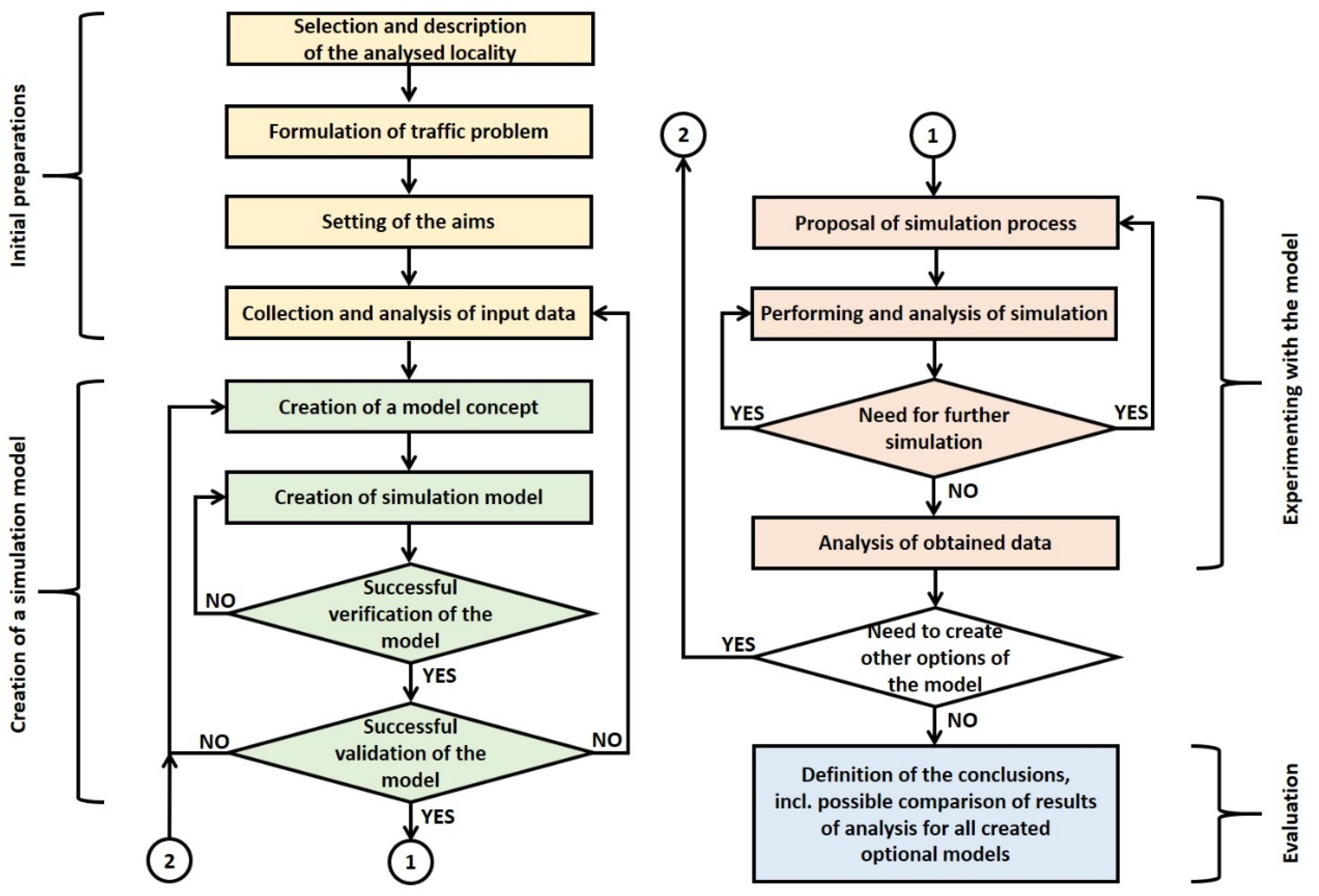
Figure 1 shows a flowchart containing individual steps of the analysis. The whole process is divided into four basic parts, i.e., the initial preparation, creation of a simulation model, experimenting with the model and evaluation.

As part of the initial preparations, it is first necessary to relevantly describe the selected locality, including the surroundings. In the next step of the analysis, traffic problems are specified, while it is necessary to decide whether a suitable solution can be found using simulation tools. The most suitable type of model (microscopic/macroscopic, dynamic/static, etc.) is also selected here. Subsequently, the basic aims that the simulation process is to follow are set. Part of this step should be to decide about optional scenarios (i.e., to define different options of the model). The last step of this part is the collection and analysis of input data. This step can take place during the process of creating the model (often the input data must also be updated).

The next part concerns the creation of the simulation model itself [76,77]. The following part concerns the creation of the simulation model itself. One of the most important steps is to create a model concept. The correct methodology for model creation is selected, and the appropriate (or required) degree of abstraction of the analysed locality is determined. Then the basic traffic skeleton of the model is modelled, which can already be loaded with traffic. Only then other systems can be inserted into the model, such as public transport, pedestrian and bicycle transport systems, etc. However, it is pointless to create an excessively large model, as any small error can significantly influence the result of the simulation. We will then create our own simulation model from the conceptual model and later perform experiments on it. It is necessary to have at least basic knowledge of the relationships between generally accepted principles of modelling and their implementation in the modelling software used. Model verification means checking and verifying the functionality of the model. The functional characteristics of the model and their accuracy, compliance with physical laws, etc., are tested. It is suitable to perform the verification already during the creation of the model. The validation of the model is confirmed by the fact that the created model corresponds to the real model and provides appropriate results with the required degree of accuracy for the given purpose of the simulation study.

After creating the model and its successful verification and validation, it is possible to start experimenting with the model [76,77]. The design of the simulation process consists of the creation of plans of simulation experiments, i.e., the determination of the number of simulation experiments, their length and the method of performance. This is followed by the actual simulation and its evaluation. This is repeated depending on the specified number of simulations. If new problems or facts appear during experimentation that need to be taken into account in the model, it is necessary to determine a new design of the simulation process. After performing all planned simulations, the analysis of the obtained data follows.

The previous two stages (i.e., model creation and experimentation) are repeated in the case of more options of the model (in the present article, these are Models A, B and C).

In the final part, the evaluation of the results of analyses and the definition of conclusions are performed. The results of the experiments can be presented using tables or graphs and, if necessary, using appropriate statistical tools, but always taking into account the purpose of the simulation study. In the case of creating more options models, a comparison of the results of the analysis for all models is performed.

5. An Analysed Locality

5.1. Description of Transit Node

The analysed transit node (called Svinov-mosty) is located in the city of Ostrava (the Czech Republic, GPS 49°49′27.105″ N, 18°12’36.807″ E; see Figure 2—position 1). It is a multi-level bridge that allows passengers to transfer between bus and tram links. This transit node is within a walking distance of the important train station Ostrava-Svinov (see Figure 2—position 2). The analysed place thus connects several types of transport, not only public transport (i.e., urban public transport, long-distance bus and train transport) but also individual car transport (in the locality, there are both a car park and a parking house; see Figure 2—positions 4 and 6). There is also a transport link from the train station to Leos Janacek Airport in Ostrava.

The transit node Svinov-mosty and its parts are shown in Figure 3, or schematically in Figure 4. The name of the transit node, i.e., Svinov-mosty, indicates the district Svinov and bridges (in Czech “mosty”). It is a system of two roads and two tram bridges. From the transport point of view, it is a three-floor construction. On the ground floor (i.e., at the level of the surrounding terrain), there are bus stops for urban and long-distance transport (Figure 3—position 6 and Figure 4—position D1 + D2). The first floor is located at a height of about 6 m, and it consists of a corridor under the structure of the bridges (Figure 3—position 5), into which individual staircases and escalators and lifts lead. It is therefore a kind of “pedestrian intersection”, where passengers are divided in all possible directions within this transit node. The second floor is at a height of about 10.5 m above the ground level and is located directly on the bridges. There are bus stops for urban and long-distance transport (Figure 3—position 1 and Figure 4—position H1–H8) and tram stops (Figure 3—position 2 and Figure 4—position T1+T2).

The diagram of the analysed transit node is shown in Figure 4. There are, among other things, obvious staircase towers, which are used for the movement of passengers between floors. These are the north staircase tower (see Figure 4—position 1, or Figure 3—position 3), the south staircase tower (see Figure 4—position 3, or Figure 3—position 7) and two internal staircase towers (see Figure 4—position 2, or Figure 3—position 9). All towers include stairs, escalators and a lift in various layouts. At the stops and pedestrian areas there are tactile guide paths, signal and warning strips according to the technical requirements for barrier-free use of the constructions.

5.2. An Extension of Tram Network

One of the tasks (see Model B below) set by this study was to verify the capacity of the analysed transit node in a case of an expansion of the tram network in the district Poruba (see Figure 5—position 2, or green colour). The new tram line will replace at least a part of some bus links or cause more significant changes, which will also affect the traffic on the monitored transit node (in Figure 5, see position 1). To describe the overall changes in the bus and tram links, changes in the numbers of connections, or cancellation or redirection of some links to other routes, etc., are not technically possible in this article, and it is not necessary. To monitor the changes within the analysed transit node, the following conclusions are sufficient, which were defined on the basis of the study of information, e.g., from [75,80,81], and which are related to bus links passing through the analysed transit node (specifically link no. 48 and 49). The new tram line will follow the route shown in Figure 5 in green colour. The route of this tram line will go partly along the existing route of bus link no. 48 and 49 (in Figure 5, the line in green-yellow colour). For this reason, some passengers from link no. 48 will use the new tram line. It is also planned to cancel part of bus link no. 49 in the section from the analysed transit node to the end of the new tram line (in Figure 5, the yellow dashed line). The other links will also be affected, but according to the available documents, this effect will not be significant. In any case, passengers currently travelling from the city centre to the districts Poruba and Pustkovec (see Figure 5) will not have to change (at the analysed transit node) from tram to bus, but will be able to continue by tram. Thus, there will be a decrease in transfers between buses and trams at the transit node, but among other things, the numbers of passengers at tram stops, which will offer new travel options, will change.

6. Traffic Surveys

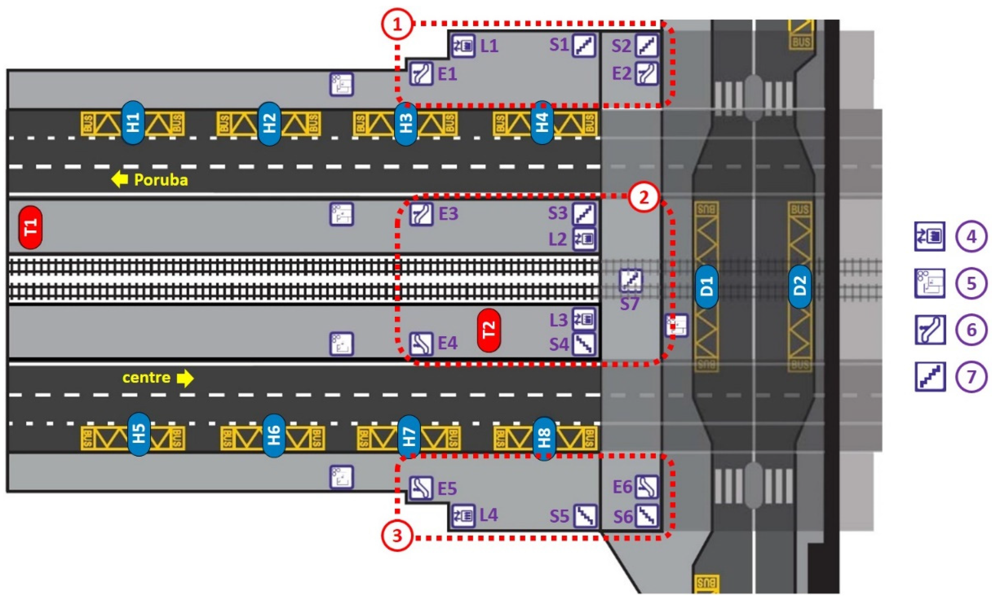
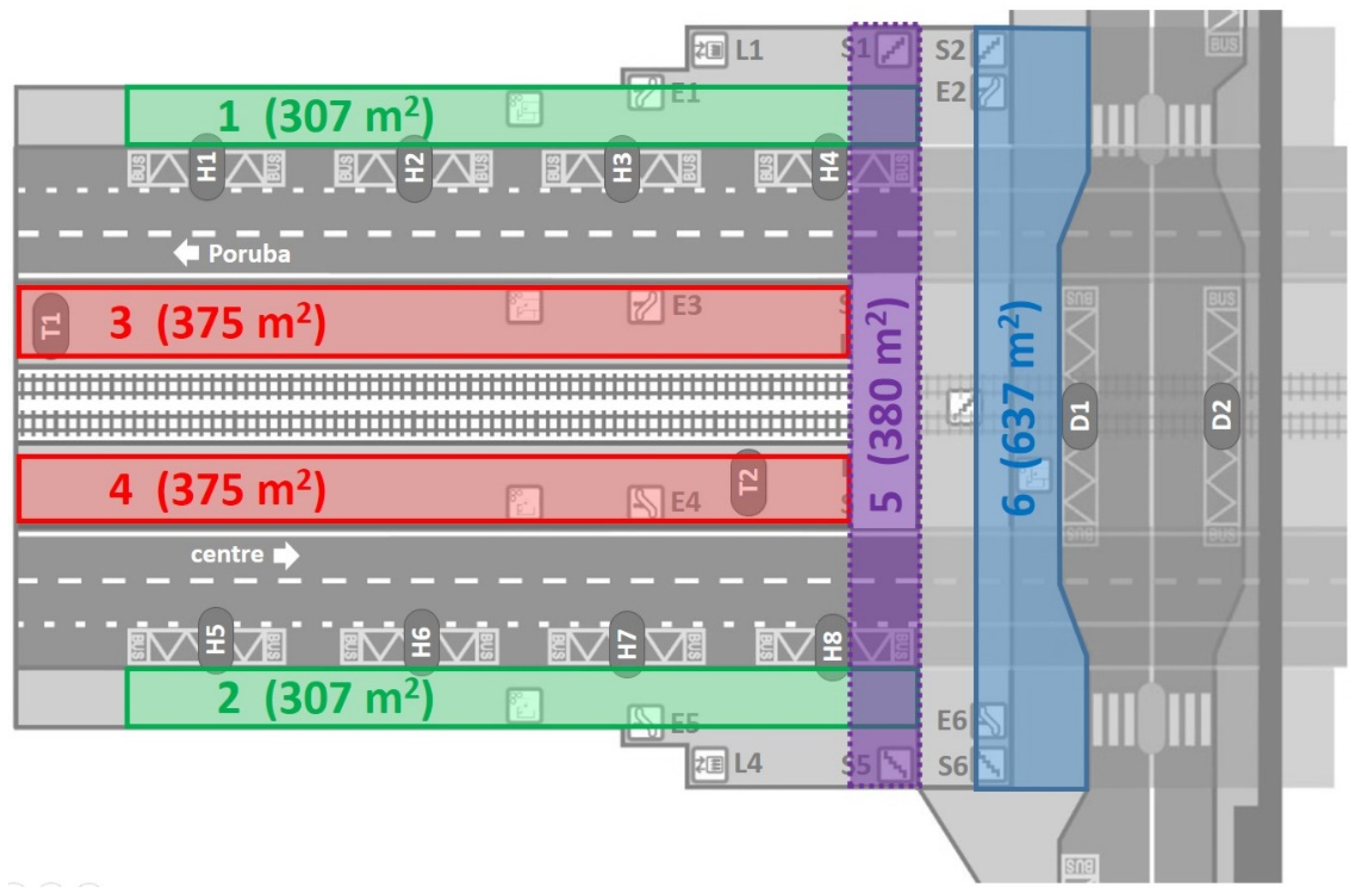
The basic input data for the analyses were pedestrian volumes. Passengers can enter the monitored transit node areas in two ways, i.e., they come from the surrounding area or arrive by public transport vehicles. From the surrounding area, passengers can come from the north (i.e., in the place of the northern staircase tower—see Figure 4, position 1), or from the south (i.e., in the place of the southern staircase tower—see Figure 4, position 3). These places were subsequently defined in the traffic model as the so-called pedestrian inputs. The pedestrian volumes found by the research in the afternoon peak hour are stated in

Table 1. The intensities of pedestrians entering the model from the surrounding area (3 p.m.–4 p.m.).

Pedestrian Input	300–315 p.m.	315–330 p.m.	330–345 p.m.	345–400 p.m.	Total
North	120	127	50	57	354
South	155	170	120	170	615
Total	275	297	170	227	969

.

Traffic volumes of departing and boarding passengers were obtained from the data obtained by the company KODIS [79], or from [75]. These were passengers of urban and long-distance bus links, as well as passengers of tram links. Due to copyright, a sample of the data obtained cannot be published in this article. Therefore, we limit ourselves to a verbal description. The direction and number of the link, the time of the connection, the number of passengers who arrived, disembarked, boarded and departed, and the maximum vehicle occupancy and its capacity utilization in percentage were stated for each connection of the given transport link. Regarding the number of connections, for example, in the afternoon peak hours on a working day (3 p.m.–4 p.m.), 36 tram connections were recorded in the direction to the district Poruba (see Figure 4—position T1), 37 tram connections in the direction to the city centre (see Figure 4—position T2), 32 bus connections in the direction to Poruba (see Figure 4—position H1–H4) and 34 bus connections in the direction to the city centre (see Figure 4—position H5–H8). From the stops on the ground floor of this transit node, 22 connections departed from stop D1 and 16 connections departed from stop D2 (see Figure 4—position D1 + D2). For illustration, we present the number of transport links that pass through the relevant stops (as indicated in Figure 4): T1—5 links, T2—5 links, H1—1 link, H2—3 links, H3—3 links, H4—1 link, H5—1 link, H6—1 link, H7 –3 links, H8—3 links, D1—14 links and D2—13 links (stops H1 and H5 are served mainly by the long-distance links; a larger number of long-distance links is also at stops D1 and D2).

These data had to be supplemented by our own traffic surveys, which focused on the transfers of passengers between individual means of transport (or between individual floors of the transit node) during transfers from link to link. In other words, it was necessary to analyse the movements of passengers between floors, the usage of stairs, escalators and lifts, etc. For this purpose, informed people were used. They conducted the census. Video cameras were also used. Due to the large content of the obtained data, we limit the discussion to only the sample shown in

Table 2. An example of the results of a traffic survey: numbers of passengers using staircases (S1–S7) and escalators (E1–E6) during afternoon maximum peak hour.

Time	S1	S2	S3	S4	S5	S6	S7	E1	E2	E3	E4	E5	E6
300–315 p.m.	0	14	4	0	24	27	21	56	118	96	108	54	90
	8	33	14	15	19	15	13	59	81	121	43	53	85
315–330 p.m.	1	25	1	0	13	0	15	55	92	38	44	20	17
	3	30	10	1	7	2	8	45	76	105	32	23	56
330–345 p.m.	0	12	1	0	16	5	4	58	153	38	73	40	52
	1	40	15	17	9	0	1	44	98	110	35	42	62
345–400 p.m.	0	30	0	0	17	4	9	49	102	41	83	22	65
	5	22	5	18	5	0	11	30	65	45	43	20	25
Subtotal	1	81	6	0	70	36	49	218	465	213	308	136	224
	17	125	44	51	40	17	33	178	320	381	153	138	228
Total	18	206	50	51	110	53	82	396	785	594	461	274	452

The upper value indicates the number of people upwards, the lower value downwards. The subtotal and total values are in person per hour. For designations S1–S7 and E1–E6, see Figure 4.

. The table shows the number of passengers using stairs S1–S7 and escalators E1–E6 (see Figure 4 for designation), again during the afternoon peak hours (3 p.m.–4 p.m.), which was eventually used in a microsimulation traffic model. Greater usage of escalators is evident (compared to staircases), as due to the importance of this transit node, there are a larger number of passengers with larger luggage (suitcases, etc.). Due to the minimal usage of lifts (on average, 4 people/h per lift), the capacities of the lifts were not evaluated in the analyses.

The traffic model also needed to take into account the composition of pedestrian traffic, which is closely related to walking speed. The usual walking speed of a healthy adult on a plain is about 5 km/h. However, this problem is not so clear-cut. It is necessary to take into account, for example, the proportion of older people, people with special needs, etc. The PTV VISSIM/VISWALK program uses the so-called speed distribution function, which takes into account the age of the pedestrians and their possible reduced mobility.

Table 3. Division of pedestrians according to the speed of movement, age and other attributes according to PTV VISSIM/VISWALK [63].

Pedestrian Class	Sex	Speed (km/h) (Lower Bound)	Speed (km/h) (Upper Bound)	Percentage in Models (%)
<30	Male	4.00	6.66	12.3	27.4
	Female	3.35	5.58	15.1
30–50	Male	3.49	5.83	22.7	46.3
	Female	2.56	4.28	23.6
>50	Male	3.02	5.04	6.8	15.7
	Female	2.02	3.38	8.9
With Reduced Mobility	Male	2.30	3.82	4.1	7.8
	Female	1.55	2.56	3.7
With Severely Reduced Mobility	Male	1.98	3.28	1.6	2.8
	Female	1.33	2.20	1.2

shows the lower and upper speed limits for the individual pedestrian classes as well as the percentages used in the analysed models. These percentages were determined on the basis of video recordings taken as a part of traffic surveys. Since transport is basically a stochastic system, these adjustments are sufficient for the needs of the described analyses. The real speed of movement of individual pedestrians is naturally influenced (usually reduced) in the model by a number of factors, e.g., avoiding obstacles and other pedestrians, taking the stairs or using escalators, etc.

For the needs of traffic models, it was also necessary to find out the number of car transport vehicles that pass on roads and can affect departures of buses from stops. The volume of vehicles passing bus stops on the 2nd floor (i.e., H1–H8—see Figure 4) is about 5000 vehicles per peak hour. The volumes of vehicles at stops D1 + D2 on the ground floor is basically negligible (approx. 100 veh/h).

7. Evaluation of the Capacity of the Transit Node According to the Technical Standards

No technical conditions or technical standards deal with the issue of the evaluation of the capacity of transit nodes in the Czech Republic in more detail. For the purposes of determining the capacity, the Czech standard CSN 73 6110 Design of Urban Roads [82] was used. It describes the capacity of roads for pedestrians. Furthermore, the standard CSN EN 115 Safety of Escalators and Moving Walkways [83], which, among other things, specifies the procedure for determining the capacity of escalators, was also used.

7.1. Evaluation of Pedestrian Areas

For the evaluation of the capacity of the analysed transit node, first it was necessary to determine the so-called Level of Service (LoS) of areas designated for pedestrians. For this purpose, the sizes of pedestrian areas were measured using project documentation in DWG format and using AutoCAD Civil 3D. These were the areas of bus and tram platforms, connecting the corridor and the space on the ground floor (see Figure 6, where the approximate positions of these areas are drawn).

The Level of Service (LoS) for pedestrian areas is evaluated according to CSN 73 6110 [82] and is similar to the evaluation of LoS for vehicles. As with vehicles, LoS in pedestrians expresses the comfort of their movement on the road. The basic determining criterion is the pedestrian speed of movement, which is closely related to the pedestrian traffic density. With increasing volume and density of pedestrians, the speed decreases and the freedom of movement is reduced. The walking speed of approx. 2.5 km/h is unnaturally slow and corresponds to a density of 1.3–1.7 person/m² [82]. At a density of 0.7 person/m² and more, the speed increases to only 3.0–3.5 km/h (in this state, even slow pedestrians must reduce their speed of movement) [82]. Only at 0.25 person/m² and less, the fastest pedestrian can reach speeds of up to approx. 6.5 km/h [82]. Further details, which will be used later in the analysis of the results from microsimulation traffic models, are given in

Table 4. Level of Service for the movement of pedestrians on the pedestrian areas. Modified from [82].

Level of Service	Average Density (pedestrians/m2) Capacity (pedestrians/h/lane)	Description
A	0.08 120–180	The pedestrian moves freely, at the chosen speed, without conflicts.
B	0.27 240–36	The movement is still free. The effect of the presence of other pedestrians is small.
C	0.46 600–900	Possibility of both walking at normal speed and overtaking in one direction. Minor conflicts in cross or opposite movement. Slight reduction in speed.
D	0.71 900–1300	The choice of speed and overtaking is limited. Cross and opposite movements require changes in speed and position and are conflicting. Perceptible interactions between pedestrians.
E	1.67 1500–2200	Significant limitation of speed; overtaking is not possible. Cross and opposite movements only with great difficulty. Limit state of capacity with interruption to stopping of movement.
F	>1.7 variable	Movement is unstable and possible only very slowly. Constant contact with other pedestrians. Cross and opposite movements are impossible. The state is approaching a cluster of pedestrians without movement.

. It describes, among other things, the individual degrees of LoS, which are marked with the letters A to F.

Technical standard CSN 73 6110 [82] also specifies the Level of Service for so-called pedestrian clusters (e.g., at public transport stops). On the basis of the average number of people per square meter, the individual degrees of Level of Service are determined. A more detailed description is given in

Table 5. Level of Service for pedestrians in clusters. Modified from [82].

Level of Service	Average Number of People/m2	Average Area (m2/person)	Description
A	0.75	1.40	Standing or free movement are possible without mutual interference.
B	1.00	1.00	It is possible to stand, and movement is partially limited without mutual interference.
C	1.40	0.70	Standing and limited movement is possible with mutual interference. Density is within the limits of personal comfort. Heavily loaded transfer stations.
D	2.50	0.40	Standing is possible without touching each other. Movement is significantly limited, and forward movement is only possible in a group. Very heavily loaded transfer stations.
E	4.00	0.25	Physical contact with other people is inevitable. Movement inside the cluster is impossible. Only for short-term peak hours (sports matches, etc.).
F	>4.00	<0.25	All people are in direct physical contact. No movement is possible. The density is very uncomfortable. Crowded public transport vehicles and lifts.

.

7.2. Evaluation of Escalators

The maximum capacity of escalators C_e,max is given by the standard CSN EN 115 [83] (

Table 6. Maximum capacity of escalators C_e,max according to CSN EN 115. [83].

Belt Width	Nominal Speed (m/s)
(m)	0.50	0.65	0.75
0.60	3600 persons/h	4400 persons/h	4900 persons/h
0.80	4800 persons/h	5900 persons/h	6600 persons/h
1.00	6000 persons/h	7300 persons/h	8200 persons/h

).

The capacity of the escalators of the analysed transit node was subsequently evaluated using the volume-to-capacity ratio:

$$a_v=\frac{I_e}{C_{e,max}} [-]$$

(1)

where I_e is the volume of pedestrians on escalators (persons/h) and C_e,max is the maximum capacity of the escalator given by the standard CSN EN 115 (persons/h) (see Table 6).

The evaluation of the capacity of the escalators then consists in the determination of the capacity reserve, which must reach at least positive values. The capacity reserve of escalators is determined from the relation

$$R=I_e-C_{e,max}(\mathrm{persons}/\mathrm{h})\mathrm{or}R=\left(1-\frac{I_e}{C_{e,max}}\right)\times 100 [\%].$$

(2)

From the above-mentioned formula, it is obvious that both parameters, i.e., volume-to-capacity ratio a_v and capacity reserve R (in decimal form, which we get by dividing R in % by the number 100), after the mutual sum, give the result equal to 1.

There are escalators with a width of 0.80 m in the observed transit node, which move at the nominal speed of 0.50 m/s. From Table 6, it follows that their maximum capacity C_e,max is 4800 persons/h.

7.3. Evaluation of Staircases

In technical standard CSN 73 6110 [82], the capacity of staircases is defined more or less vaguely. It is stated here that the capacity of staircases compared to pedestrian areas decreases to at least 0.65 times the values given in Table 4. If the staircases are, for example, in railway stations, where pedestrians with luggage often move, the values from this table fall below 50%. Capacity is also reduced by the length of the staircase (i.e., the increasing height to be overcome, as in higher parts of the staircases the pedestrians tend to be tired and they slow down)—this applies mainly to staircases that have the difference of height of more than 10 m.

In the performed analyses, for the above-mentioned reason, the staircases are evaluated only with the use of microsimulation models.

8. Microsimulation Traffic Models

8.1. Used Software

The specialized software PTV VISSIM, together with PTV VISWALK, was used to create a microsimulation traffic model of the analysed transit node. Both programs use a common software environment, so in the following text, the designation PTV VISSIM/VISWALK is also used.

For the purposes of the analysis of pedestrian movement in the monitored transit node, three models representing different states of traffic load were created (for more details, see other subsections):

• Model A—a model of normal state, i.e., at normal load;
• Model B—a model taking into account the new tram line;
• Model C—a model at full (extraordinary) load.

8.2. Model A—A Model of Normal State

As a model representing the normal state of traffic at the analysed transit node (i.e., the movement of the vehicles of road traffic, vehicles of public transport and pedestrians), a model for afternoon peak hour was created. The drawing shown in Figure 7 was used as a plan view.

On the basis of the plan view and the knowledge of height parameters of individual floors, a 3D model of transit node was created in the PTV VISSIM/VISWALK program (in the following text, the names of the so-called objects of modelled transport network (Network Objects) are marked in italics). The model itself consists of, among other things, roads and tram lines (Links) at various height levels, areas for pedestrians (Areas), stairs and escalators (Ramps & Stairs—the program allows you to model inclined ramps) and obstacles such as columns (Obstacles). Objects of Public Transport Lines and Public Transport Stops were used for public transports routes and stops.

The resulting 2D model is shown in Figure 8, with the left image (a) showing the model in full view, while the right image (b) shows it in a simplified view, i.e., the so-called toggle wireframe. The model in 3D is shown in Figure 9.

The model of the transit node was subsequently loaded with the appropriate volumes of vehicles and pedestrians (Vehicle Inputs and Pedestrian Inputs) and the routes they use (Vehicle Routes and Pedestrian Routes) were determined. Figure 10 shows an example of pedestrian movement between individual points of interest, i.e., between entrances to the model, staircases and escalators, bus and tram stops, etc. (see yellow lines). In the right part of Figure 10, there is an example of the entered data, including selected attributes.

Figure 11 shows an example of an already running simulation in the created model. During the simulation, among other things, the time of transfer of passengers between points of interest (Pedestrian Travel Times) was monitored and a comparison of these times between individual models was performed (i.e., Models A, B and C—see below).

The results from the analyses of Model A are presented in Section 9.2.

8.3. Model B—A Model Taking into Account the New Tram Line

As mentioned above, it is planned to expand the tram network in the district Poruba (see Figure 5). The construction of a new tram line will also affect the situation at the monitored transit node. The created transport model was, therefore, modified to respect the changes described above (i.e., the transfer of part of the passengers between the individual bus and tram links, the cancellation of one bus link, etc.).

The results of this analysis are stated in Section 9.3.

8.4. Model C—A Model at Full Load

The last model simulated the situation of full (extraordinary) load. It was a theoretical simulation of a situation that occurs, e.g., as a result of extraordinary social or sports events. During these events, only the traffic volumes in some directions are usually increased, but to determine the theoretical capacity at full load, all pedestrian volumes from Model A were increased four times. The number of chosen connections was also increased (e.g., during special events, so-called additional connections are usually added to chosen links). Subsequently, it was monitored whether the analysed transit node is able to handle this load.

The results of this analysis are stated in Section 9.4.

9. The Results of Analyses

9.1. Monitored Parameters

For the analysed transit node, the following evaluation (the numbering of the following subsections corresponds to the subsection numbers, which are used in the following text for individual models) was performed for each model (i.e., Models A, B and C—see Section 8.2, Section 8.3 and Section 8.4). As mentioned earlier, the models used data from traffic surveys during the afternoon peak hours (i.e., from 3 p.m. to 4 p.m.).

9.1.1. Evaluation of Pedestrian Areas

On the basis of the results from microsimulation models created in PTV VISSIM/VISWALK, the Level of Service (LoS) was determined for pedestrian areas in two ways. First, all pedestrian areas (i.e., nos. 1–6 according to Figure 6) were evaluated in terms of movement of pedestrians in these areas (according to Table 4). Then, the areas that contain stops (i.e., nos. 1–4 and no. 6 according to Figure 6), were evaluated in terms of the movement of pedestrian in the cluster (according to Table 5).

During the evaluation of the model, among others, some parameters were monitored, which are defined according to [63] as follows:

• density (persons/m²)—density of pedestrians on areas, escalators and staircases;
• perceived density (person/m²)—density of pedestrians perceived around the pedestrian, i.e., the number of other pedestrians around the pedestrian;
• speed (km/h)—average pedestrian speed calculated as harmonic average.

The simulation of vehicle and pedestrian traffic in the analysed transit node lasted one hour for each model. However, the PTV VISSIM/VISWALK program records data in seconds and, therefore, the simulation length is defined as 3600 s. However, the evaluation of data from the model always started only in the tenth minute of the simulation (i.e., in the time 600–3600 s (see graphs below)) due to the gradual loading of the model by volumes of vehicles and pedestrians (up to 600th second the program gives relevant data).

9.1.2. Evaluation of Escalators

Escalators are also a part of the analysed transit node. There is a total of six pairs of escalators (each pair allows the movement of people in both directions). Here, too, the escalators were evaluated in two ways. First, Level of Service was determined in the same way as in the case of the movement of pedestrians on pedestrian areas (i.e., according to Table 4). Then the escalators were evaluated on the basis of the capacity reserve according to Table 6, or Formulas (1) and (2).

Each escalator has a belt width of 0.8 m and a nominal speed of 0.5 m/s. The lengths of the escalators vary depending on the overcome height. Therefore, the maximum capacity of the escalator configuration used is, according to Table 6, 4800 persons/h. However, a prerequisite for such capacity is the smooth occupation of the belt by passengers. In reality, however, passengers usually keep certain distances between themselves, which reduces capacity. In addition, many passengers have large luggage, or animals, bicycles, etc., which again reduces the real capacity. Passengers with reduced mobility enter the escalator more carefully and slowly.

9.1.3. Evaluation of Staircases

As mentioned earlier, standard CSN 73 6110 defines staircase capacity very briefly. Therefore, the staircases were evaluated in the same way as pedestrian areas and escalators, i.e., by determination of the Level of Service according to Table 4.

9.1.4. Evaluation of Travel Times

The analysed transit node allows for a number of movements of passengers, such as moving from the edges of the model to a bus/tram stop, and vice versa, or transfers between individual bus/tram links. The results obtained from the microsimulation models showed that for the capacity evaluation of the analysed transit node, it is necessary to analyse in more details the so-called travel time of passengers from the edges of the model to stops, and vice versa. According to [63], the travel time (s) is defined as an average pedestrian travel time from the starting area to the destination area (e.g., from entering the model to reaching the desired stop). The edge of the model for the analysed transit node was represented by area no. 6 (see Figure 6) and bus/tram stops (in Figure 6, areas 1 to 4). The individual routes were marked as d1–d4 for routes leading from areas 1–4 down to area no. 6 and as u1–u4 for routes leading from area no. 6 up to area nos. 1–4. It is clear from Figure 4 that for each route, the passenger could use different escalators or staircases to move between the areas.

Travel times between stops on the 2nd floor (i.e., between areas 1 to 4) did not show a significant problem in terms of capacity, and therefore the results will not be reported here.

9.2. Model A—A Model of Normal State

9.2.1. Evaluation of Pedestrian Areas

Table 7. Level of Service of movement of pedestrians on pedestrian areas (Model A).

Area 1	Density (person/m2)	Perceived Density (person/m2)	Speed (km/h)	Level of Service (LoS)
1	0.03	2.19	0.50	A
2	0.01	0.02	1.06	A
3	0.02	0.04	1.91	A
4	0.01	0.02	2.25	A
5	0.01	0.05	3.63	A
6	0.01	0.02	3.36	A

¹ See Figure 6.

shows the detected densities of pedestrians, including perceived densities, average walking speed and especially the level of LoS. The model, which was loaded with normal traffic volumes, shows degree A in all observed pedestrian areas, i.e., free movement of pedestrians without mutual conflicts and by chosen speed of walking.

It is clear from the result that the areas of bus and tram platforms (areas no. 1–4) show lower speeds than, e.g., area no. 5 (walk-through corridor), which serves only for transfers of passengers and not for waiting for the bus/tram connection.

The course of changes in densities of pedestrians over time is shown in the graph in Figure 12 (as explained above, the analyses took place over a time of 600–3600 s). Both from Table 7 and from this graph, it is obvious that the highest density values were reached on areas 1 and 3 or, from the more detailed analyses shown in the graph, also area 5. However, as already mentioned, these values are so small that it can be stated that in Model A, the analysed pedestrian areas are satisfactory in terms of capacity.

The results of the evaluation of LoS for pedestrians in the cluster are shown in

Table 8. Level of Service for pedestrians in clusters for maximum peak hour (Model A).

Area 1	Surface Area [m2]	Volume [person/h]	Average Number of People/m2	Average Area (m2/person)	Level of Service (LoS)
1	307	414	1.35	0.47	C
2	307	254	0.83	1.21	B
3	375	594	1.58	0.63	D
4	375	461	1.23	0.81	C
6	637	1597	2.51	0.40	D
Overall degree of LoS:					D

¹ See Figure 6.

. As described in Table 5 the areas of stops should correspond to the degree C or better. The results of the analysis show that both bus platforms (areas no. 1 and 2) and one of the tram platforms (area no. 4) meet the requirement for sufficient LoS (i.e., degree C or B). The second tram platform (area no. 3) and the area on the ground floor with the bus stop (i.e., area no. 1) already show LoS at degree D. The final degree of LoS for the analysed transit node is given by the worst degree of LoS of the observed areas, i.e., in this case D (i.e., according to areas no. 3 and 6).

From what is mentioned above, it follows that the transit node does not meet the requirements of the required level of LoS during peak hours. However, it must be taken into account that the course of pedestrian volumes is usually not uniform in the case of transit nodes. There are some waves of moving people, which are caused by the arrival of public transport vehicles. Passengers who get out of the vehicle will then and temporarily increase the current volume of pedestrians, which after a certain time will decrease again after the dispersal of passengers. Standard CSN 73 6110 [82] allows for these cases the evaluation of the capacity of the transfer node using a 15 min peak. In this case, the resulting degrees of LoS are significantly more favourable, as shown in

Table 9. Level of Service for pedestrians in the cluster for a 15 min peak (Model A).

Area 1	Surface Area (m2)	Volume (persons/15 min)	Average Number of People/m2	Average Area in m2/Person	Level of Service (LoS)
1	307	148	0.48	2.07	A
2	307	108	0.35	2.84	A
3	375	150	0.40	3.64	A
4	375	177	0.31	5.60	A
6	637	459	0.72	1.39	A
Overall degree of LoS:					A

¹ See Figure 6.

. It is clear from the results that all areas reach degree A, i.e., that they meet the requirements for the minimum degree C of LoS. When evaluating capacity with this permitted procedure, the analysed transit node complies with the capacity.

9.2.2. Evaluation of Escalators

Regarding the analysis of density on escalators, the densities of pedestrians are slightly higher compared to pedestrian areas (which can be explained due to the tighter dimensions of escalators)—see

Table 10. Level of Service of escalators (Model A).

Escalator 1	Density (person/m2)	Perceived Density (person/m2)	Level of Service (LoS)
E1-up	0.05	0.01	A
E1-down	0.20	0.27	B
E2-up	0.09	0.03	B
E2-down	0.24	0.16	B
E3-up	0.11	0.04	B
E3-down	0.13	0.08	B
E4-up	0.08	0.03	A
E4-down	0.12	0.08	B
E5-up	0.03	0.01	A
E5-down	0.11	0.18	B
E6-up	0.04	0.01	A
E6-down	0.18	0.12	B

¹ See Figure 4.

. However, the Level of Service still reaches sufficient degrees A and B, i.e., again free movement with minimum effect of the presence of other pedestrians. An interesting attribute is the perceived density, which indicates the number of people in the vicinity of a given pedestrian, i.e., the number of passengers perceived in the immediate surroundings. Its value is the highest for the escalator E1 leading from the bus stops H1–H4 (see Figure 4) downwards, i.e., from the 2nd floor to the connecting corridor on the 1st floor. In general, we can state that in Model A, the analysed escalators are satisfactory in terms of capacity.

The results of the analysis of escalator capacity reserves are shown in

Table 11. Capacity reserve of the escalators (Model A).

Escalator 1	Ie (persons/h)	av (–)	R (persons/h)	R (%)
E1-up	218	0.045	4582	95.5
E1-down	178	0.037	4622	96.3
E2-up	465	0.097	4335	90.3
E2-down	320	0.067	4480	93.3
E3-up	213	0.044	4587	95.6
E3-down	381	0.079	4419	92.1
E4-up	308	0.064	4492	93.6
E4-down	153	0.032	4647	96.8
E5-up	136	0.028	4664	97.2
E5-down	138	0.029	4662	97.1
E6-up	224	0.047	4576	95.3
E6-down	228	0.048	4572	95.3

¹ See Figure 4.

. From the last column of the table, it is evident that the capacity reserves at the maximum capacity for the used escalator configuration (i.e., 4800 persons/h—see above) are at least 90 percent. Therefore, it can be stated that even with a real reduced capacity caused often by only partial usage of escalators (distancing, luggage, etc.—see above), the capacity reserve of escalators will still be sufficient.

9.2.3. Evaluation of Staircases

As already shown from the performed traffic surveys, the traffic volumes on fixed staircases are relatively low, from which it can be assumed that the density of people on the staircases will also be negligible.

Table 12. Level of Service of staircases (Model A).

Staircase 1	Density (person/m2)	Perceived Density (person/m2)	Speed (km/h)	Level of Service (LoS)
S1	0.01	0.02	3.25	A
S2	0.01	0.00	3.54	A
S3	0.01	0.01	3.23	A
S4	0.00	0.00	4.21	A
S5	0.00	0.00	2.93	A
S6	0.01	0.01	3.14	A
S7	0.01	0.01	3.24	A

¹ See Figure 4.

shows the densities of pedestrians, including the perceived densities, average speeds of walking on staircases, and especially the degrees of LoS. The Level of Service shows degree A for all monitored staircases, i.e., free movement of pedestrians without mutual conflicts and by chosen speed of walking. It ranges from 3.14 km/h to 4.21 km/h. Thus, even in the case of fixed staircases, it can be stated that they are satisfactory in terms of capacity within Model A.

9.2.4. Evaluation of Travel Times

Table 13. Analysis of travel times (Model A).

Designation of Routes	Initial Area 1	Final Area1	Direction of Walking	Average Travel Time [s]	Number of Pedestrians [person/h]
d1	1	6	down	84.85	164
d2	2	6	down	62.62	88
d3	3	6	down	127.79	131
d4	4	6	down	104.84	130
u1	6	1	up	70.1	37
u2	6	2	up	116.8	15
u3	6	3	up	86.77	76
u4	6	4	up	120.93	52

¹ See Figure 6.

shows the average travel times found from the microsimulation traffic model, including the number of pedestrians using the relevant route. Average travel times range from about 1 to 2 min (or 60 to 120 s), which is not a significant problem for the analysed transit node in terms of capacity, and it corresponds to reality. In terms of the analysis of travel times, it can be stated that Model A is suitable.

9.3. Model B—A Model Taking into Account the New Tram Line

9.3.1. Evaluation of Pedestrian Areas

Model B took into account the situation affected by the construction of the planned new tram line (see above). Compared to Model A, this model respected certain changes, such as the transfer of part of the passengers between individual bus and tram lines, the cancellation of one bus link, etc. The way of analysis was identical to that of Model A.

Table 14. Level of Service for movement of pedestrians on pedestrian areas (Model B).

Area 1	Density [person/m2]	Perceived Density [person/m2]	Speed [km/h]	Level of Service (LoS)
1	0.03	1.1	0.44	A
2	0.01	0.04	0.77	A
3	0.02	0.05	2	A
4	0.01	0.02	2.28	A
5	0.01	0.04	3.62	A
6	0.01	0.03	3.3	A

¹ See Figure 6.

shows the detected pedestrian densities, including perceived densities, average walking speed and degrees of LoS. It was found that Model B also shows degree A in all observed pedestrian areas, i.e., free movement of pedestrians without mutual conflicts and by chosen speed of walking.

There were no significant changes in densities on the observed areas compared to the previous model. Densities have slightly increased in areas 1 and 3, i.e., stops for transport links in the direction of Poruba, where a new tram line is to be designed. The models were analysed during the afternoon peak hour, when there is an increased transfer of people from the centre to the district of Poruba. This circumstance is also affected by the redistribution of passengers from the cancelled bus link to the tram.

The course of changes in the densities of pedestrians over time is shown in the graph in Figure 13 (as explained above, the analyses took place over a time of 600–3600 s). Both Table 14 and this graph show that the highest density values were in areas 1 and 3. However, as already mentioned, these values are so small that it can be stated that in Model B the analysed pedestrian areas are satisfactory in terms of capacity.

The results of the LoS evaluation for pedestrians in the cluster are shown in

Table 15. Level of Service for pedestrians in the cluster for maximum peak hour (Model B).

Area 1	Surface Area (m2)	Volume (persons/h)	Average Number of People/m2	Average Area (m2/person)	Level of Service (LoS)
1	307	398	1.30	0.77	C
2	307	201	0.65	1.53	D
3	375	601	1.60	0.62	D
4	375	528	1.41	0.71	D
6	637	1429	2.24	0.45	C
Overall degree of LoS:					D

¹ See Figure 6.

(for peak hour) and in

Table 16. Level of Service for pedestrians in the cluster for a 15 min peak (Model B).

Area 1	Surface Area (m2)	Volume (persons/15 min)	Average Number of People/m2	Average Area (m2/person)	Level of Service (LoS)
1	307	112	0.36	2.74	A
2	307	65	0.21	4.72	A
3	375	152	0.41	2.47	A
4	375	139	0.37	2.70	A
6	637	397	0.62	1.60	A
Overall degree of LoS:					A

¹ See Figure 6.

(for a 15 min peak). Compared to Model A, the LoS deteriorated in some areas for the peak hour, but generally the LoS is also at degree D. In the 15 min peak analysis, the LoS values are the same as for Model A at degree A.

9.3.2. Evaluation of Escalators

In the case of analysis of escalators, some minor changes can be observed compared to Model A—see

Table 17. Level of Service of escalators (Model B).

Escalator 1	Density (person/m2)	Perceived Density (person/m2)	Level of Service (LoS)
E1-up	0.03	0.00	A
E1-down	0.16	0.27	B
E2-up	0.09	0.02	B
E2-down	0.25	0.16	B
E3-up	0.10	0.03	B
E3-down	0.16	0.09	B
E4-up	0.09	0.02	B
E4-down	0.13	0.10	B
E5-up	0.04	0.01	A
E5-down	0.10	0.17	B
E6-up	0.04	0.01	A
E6-down	0.19	0.11	B

¹ See Figure 4.

. However, the density still remains relatively low and the Level of Service still reaches sufficient degrees A and B, i.e., again free movement with minimum impact of other pedestrians. Here, too, it can be stated that within the Model B, the analysed escalators are satisfactory in terms of capacity.

The capacity reserves of escalators are stated in

Table 18. Capacity reserves of escalators (Model B).

Escalator 1	Ie (persons/h)	av (–)	R (persons/h)	R (%)
E1-up	198	0.041	4602	95.9
E1-down	149	0.031	4651	96.9
E2-up	458	0.095	4342	90.5
E2-down	280	0.058	4520	94.2
E3-up	278	0.058	4522	94.2
E3-down	405	0.084	4395	91.6
E4-up	358	0.075	4442	92.5
E4-down	198	0.041	4602	95.9
E5-up	120	0.025	4680	97.5
E5-down	117	0.024	4683	97.6
E6-up	201	0.042	4599	95.8
E6-down	197	0.041	4603	95.9

¹ See Figure 4.

. Here, too, these reserves are at least 90 percent and the escalators are also satisfactory from this point of view.

9.3.3. Evaluation of Staircases

Table 19. Level of Service of staircases (Model B).

Staircase 1	Density (person/m2)	Perceived Density (person/m2)	Speed (km/h)	Level of Service (LoS)
S1	0.00	0.01	3.31	A
S2	0.01	0.01	3.53	A
S3	0.01	0.00	3.31	A
S4	0.00	0.00	3.68	A
S5	0.00	0.03	3.02	A
S6	0.01	0.01	3.12	A
S7	0.01	0.00	3.44	A

¹ See Figure 4.

shows the determined densities of pedestrians, including perceived densities, average speed of walking the staircases and degrees of LoS. The Level of Service again shows degree A for all observed staircases, i.e., free movement of pedestrians without mutual conflicts and by the chosen speed of walking. It ranges from 3.02 km/h to 3.68 km/h. Thus, even in the case of fixed staircases, it can be stated that they are satisfactory in terms of capacity within Model B.

9.3.4. Evaluation of Travel Times

Even in the case of the Model B, the travel times of passengers were from the edges of the model to stops, and vice versa (see explanation above).

Table 20. Analysis of travel times (Model B).

No. of Routes	Initial Area 1	Final Area 1	Direction of Walking	Average Travel Time (s)	Number of Pedestrians (person/h)
d1	1	6	down	86.18	148
d2	2	6	down	62.55	93
d3	3	6	down	129.18	170
d4	4	6	down	100.96	138
u1	6	1	up	83.84	28
u2	6	2	up	118.73	14
u3	6	3	up	86.64	80
u4	6	4	up	114.03	61

¹ See Figure 6.

shows the average travel times found from the microsimulation traffic model, including the number of pedestrians using the relevant route. The average travel times, similarly to Model A, range from about 1 to 2 min (or 60 to 130 s), which again does not represent a significant problem for the analysed transit node in terms of capacity. From the point of view of the analysis of travel times, it can be stated that Model B, like the previous Model A, is suitable.

9.4. Model C—A Model at Full Load

9.4.1. Evaluation of Pedestrian Areas

As mentioned earlier, the third and at the same time the last Model C was burdened with extraordinary traffic volumes, when the volumes of pedestrians were increased, as well as the number of chosen traffic connections (see details above). The method of analysis was again similar to the previous models.

Table 21. Level of Service for the movement of pedestrians on pedestrian areas (Model C).

Area 1	Density (person/m2)	Perceived Density (person/m2)	Speed (km/h)	Level of Service (LoS)
1	0.02	0.77	0.44	A
2	0.01	0.04	0.78	A
3	0.02	0.05	2.01	A
4	0.01	0.02	2.24	A
5	0.01	0.04	3.63	A
6	0.01	0.03	3.33	A

¹ See Figure 6.

shows the detected densities of pedestrians, including perceived densities, average walking speed and degrees of LoS. It was found that Model C also shows degree A in all monitored pedestrian areas, i.e., free movement of pedestrians without mutual conflicts and by chosen speed of walking.

The course of changes in the densities of pedestrians over time is shown in the graph in Figure 14 (analyses were again performed in the time 600–3600 s). It is clear from this graph that the densities decrease to zero only exceptionally. On the contrary, it reaches higher values of maximum density compared to previous models. However, even here these values are low, and it can be stated that in Model C the analysed pedestrian areas are satisfactory in terms of capacity.

The results of the evaluation of LoS for pedestrians in the cluster are shown in

Table 22. Level of Service for pedestrians in a cluster for maximum peak hour (Model C).

Area 1	Surface Area (m2)	Volume (persons/h)	Average Number of People/m2	Average Area (m2/person)	Level of Service (LoS)
1	307	1656	5.39	0.19	F
2	307	1016	3.31	0.30	E
3	375	2376	6.34	0.16	F
4	375	1844	4.92	0.20	F
6	637	6388	10.03	0.10	F
Overall degree of LoS:					F

¹ See Figure 6.

(for the peak hour) and in

Table 23. Level of Service for pedestrians in a cluster for a 15 min peak (Model C).

Area 1	Surface Area (m2)	Volume (persons/15 min)	Average Number of People/m2	Average Area (m2/person)	Level of Service (LoS)
1	307	592	1.93	0.52	D
2	307	432	1.41	0.71	D
3	375	600	1.60	0.63	D
4	375	468	1.25	0.80	B
6	637	1836	2.88	0.35	E
Overall degree of LoS:					E

¹ See Figure 6.

(for a 15 min peak). Compared to the previous models, however, there was logically a significant deterioration in LoS. In the case of the peak hour, one area showed degree E and the other degree F. Generally, LoS is also at degree F, which is of course unsatisfactory.

In the analysis of a 15 min peak, the LoS values are already more favourable, but the overall LoS is at an unsatisfactory degree E. According to Table 5, this degree of LoS involves unavoidable physical contact with other people and movement within the cluster is impossible. This condition is only possible for short-term peak hour traffic (e.g., for sports matches, etc.), which is the case with Model C.

9.4.2. Evaluation of Escalators

In the analysis of escalators in Model C, however, their density, or LoS, does not reach critical values—see

Table 24. Level of Service of escalators (Model C).

Escalator 1	Density (person/m2)	Perceived Density (person/m2)	Level of Service (LoS)
E1-up	0.03	0.00	A
E1-down	0.15	0.26	B
E2-up	0.09	0.02	B
E2-down	0.25	0.15	B
E3-up	0.11	0.03	B
E3-down	0.16	0.09	B
E4-up	0.09	0.02	B
E4-down	0.13	0.09	B
E5-up	0.04	0.01	A
E5-down	0.11	0.17	B
E6-up	0.05	0.02	A
E6-down	0.19	0.10	B

¹ See Figure 4.

. The Level of Service still reaches sufficient degrees A and B, i.e., again free movement with minimal impact of the presence of other pedestrians, although in this model, worse degree B prevails. However, it can still be stated that in Model C, the analysed escalators are satisfactory in terms of capacity.

However, the capacity reserves of escalators for the extremely loaded model are already lower than in previous models (see

Table 25. Capacity reserves of escalators (Model C).

Escalator 1	Ie (persons/h)	av (–)	R (persons/h)	R (%)
E1-up	872	0.182	3928	81.8
E1-down	712	0.148	4088	85.2
E2-up	1860	0.388	2940	61.3
E2-down	1280	0.267	3520	73.3
E3-up	852	0.178	3948	82.3
E3-down	1524	0.318	3276	68.3
E4-up	1232	0.257	3568	74.3
E4-down	612	0.128	4188	87.3
E5-up	544	0.113	4256	88.7
E5-down	552	0.115	4248	88.5
E6-up	896	0.187	3904	81.3
E6-down	912	0.190	3888	81.0

¹ See Figure 4.

), which could be assumed. The lowest value is about 60%, the highest is close to 90%. Nevertheless, it can be stated that escalators are also satisfactory in this respect.

9.4.3. Evaluation of Staircases

Table 26. Level of Service of staircases (Model C).

Staircase 1	Density (person/m2)	Perceived Density (person/m2)	Speed (km/h)	Level of Service (LoS)
S1	0.00	0.02	3.29	A
S2	0.01	0.01	3.52	A
S3	0.01	0.01	3.23	A
S4	0.00	0.00	3.68	A
S5	0.00	0.03	3.06	A
S6	0.01	0.01	3.09	A
S7	0.01	0.01	3.51	A

¹ See Figure 4.

shows the determined densities of pedestrians, including perceived densities, average speed of walking on the staircases and degrees of LoS. The Level of Service again shows degree A for all observed staircases, i.e., free movement of pedestrians without mutual conflicts and by chosen speed of walking. It ranges from 3.06 km/h to 3.68 km/h. In the case of fixed staircases, it can be stated that within Model C, they are satisfactory in terms of capacity, even in the case of significantly increased volumes of pedestrians.

9.4.4. Evaluation of Travel Times

Table 27. Analysis of travel times (Model C).

No. of Routes	Initial Area 1	Final Area 1	Direction of Walking	Average Travel Time (s)	Number of Pedestrians (person/h)
d1	1	6	down	85.89	159
d2	2	6	down	62.49	106
d3	3	6	down	129.06	200
d4	4	6	down	99.43	167
u1	6	1	up	87.64	34
u2	6	2	up	113.75	19
u3	6	3	up	87.13	99
u4	6	4	up	113.95	79

¹ See Figure 6.

shows the average travel times found from the microsimulation traffic model, including the number of pedestrians using the relevant route (for details, see previous subsections). As in the case of Model A, the average travel times range from about 1 to 2 min, which does not represent a significant problem for the analysed transit node in terms of capacity. However, the increase is noticeable (only in one case is the average travel time about 60 s; the other routes then start at about 90 s). Given that the increase in travel times at full load was nevertheless expected, there are no high values, and it can be stated that the Model C is suitable in terms of analysis of travel times.

9.5. An Overall Evaluation of the Results of Analysis for Models A, B and C

9.5.1. Evaluation of Pedestrian Areas

When evaluating the pedestrian areas of the analysed transit node in terms of pedestrian movement, it was found that all monitored areas in all three models show a Level of Service at degree A (i.e., free movement of pedestrians without conflicts and by chosen speed of walking). The obtained results are for the individual models in Table 7, Table 14 and Table 21. The time courses of the densities of pedestrians are shown in the graphs in Figure 12, Figure 13 and Figure 14 for the individual models. The densities of pedestrians change over time depending on the arriving bus/tram link. It is obvious that in Model C (i.e., full load), the values of densities of pedestrians increase. However, generally, it can be stated that in terms of the movement of pedestrians on pedestrian areas, all three models are suitable.

From the perspective of evaluation of the areas, where there are stops, and therefore, where there is a cluster of people, the situation is relatively different. When comparing the Level of Service for peak hour (see Table 8, Table 15, and Table 22), for some areas of Models A and B there is a clear deterioration in degrees of LoS up to degree D (i.e., LoS of the whole transit node is on degree D). However, the standard requires a maximum of degree C (see earlier). Model C has already, with one exception, exceeded capacity, i.e., the degree of LoS is at degree F (the total LoS is then also at degree F). These results are illustrated in the graph in Figure 15.

As mentioned earlier, the standard also allows to evaluate the clusters using a 15 min peak. The results in Table 9, Table 16 and Table 23 show that for Models A and B, the LoS drops to degree A for all areas (see Figure 16). Model C will show a relatively significant improvement (even one area has degree B), but unsatisfactory degrees of LoS still predominate. At least the finding that according to this evaluation the capacity is no longer exceeded in any area (i.e., degree F) is positive. It can be stated that in terms of evaluation of pedestrian clusters at stops, Models A and B are satisfactory. Model C, which is fully loaded, will meet the capacity, but the requirement for LoS is not fulfilled.

9.5.2. Evaluation of Escalators

Escalators could theoretically be considered one of the critical points of transit nodes. These are objects with a limited width and a limited speed of movement. However, the results of the analyses performed on the monitored transit node show that the escalators do not show major problems. Evaluation of Level of Service (see Table 10, Table 17 and Table 24) shows that a maximum of degree B is achieved for all three models (see Figure 17). The results from the evaluation of escalators according to the capacity reserve (see Table 11, Table 18 and Table 25) also show sufficient capacity (see Figure 18). It is obvious that in the first two models the capacity reserve is higher (i.e., above 90%), and in the third model it is lower (approx. 60–90%). However, even these reserves are more than sufficient. Therefore, it can be stated that the escalators of the analysed transit node are satisfactory for all three models.

9.5.3. Evaluation of Staircases

The results of the analyses of Level of Service of the staircases of the analysed transit node are given in Table 12, Table 19 and Table 26. The evaluation is very simple here. All staircases of all three models are suitable in terms of Level of Service (they reach LoS at degree A).

9.5.4. Evaluation of Travel Times

One of the important parameters that are monitored within the transit nodes are the so-called travel times. The models created in the PTV VISSIM/VISWALK program showed that travel times between stops on the 2nd floor (i.e., between areas 1 to 4—see Figure 6) did not show a significant problem in terms of capacity and were therefore not further analysed. However, the travel times between area no. 6 on the ground floor and the remaining areas on the bus/tram stops (i.e., area nos. 1 to 4) and vice versa were analysed in more detail.

The results of these analyses are for the individual models in Table 13, Table 20 and Table 27. Generally, the average travel times range from about 60 to 130 s (see Figure 19). It can be seen that, with a few exceptions, the travel times for individual routes (d1–d4, u1–u4) reach similar values without distinguishing a specific model.

The analysed travel times do not represent a problem in terms of movement between individual areas, and therefore it can be stated that the analysed transit node in terms of travel time of pedestrians is satisfactory.

10. Discussion and Conclusions

The article uses a specific example of complex transit node between bus and tram transport to analyse the transfers of passengers using a microsimulation traffic model created in the PTV VISSIM/VISWALK program. The created model was loaded in three ways: Model A with normal vehicle and passenger volumes, Model B took into account the extension of the existing tram network by a new line, and Model C, which was loaded with extraordinary volumes that may occur during cultural or sports events.

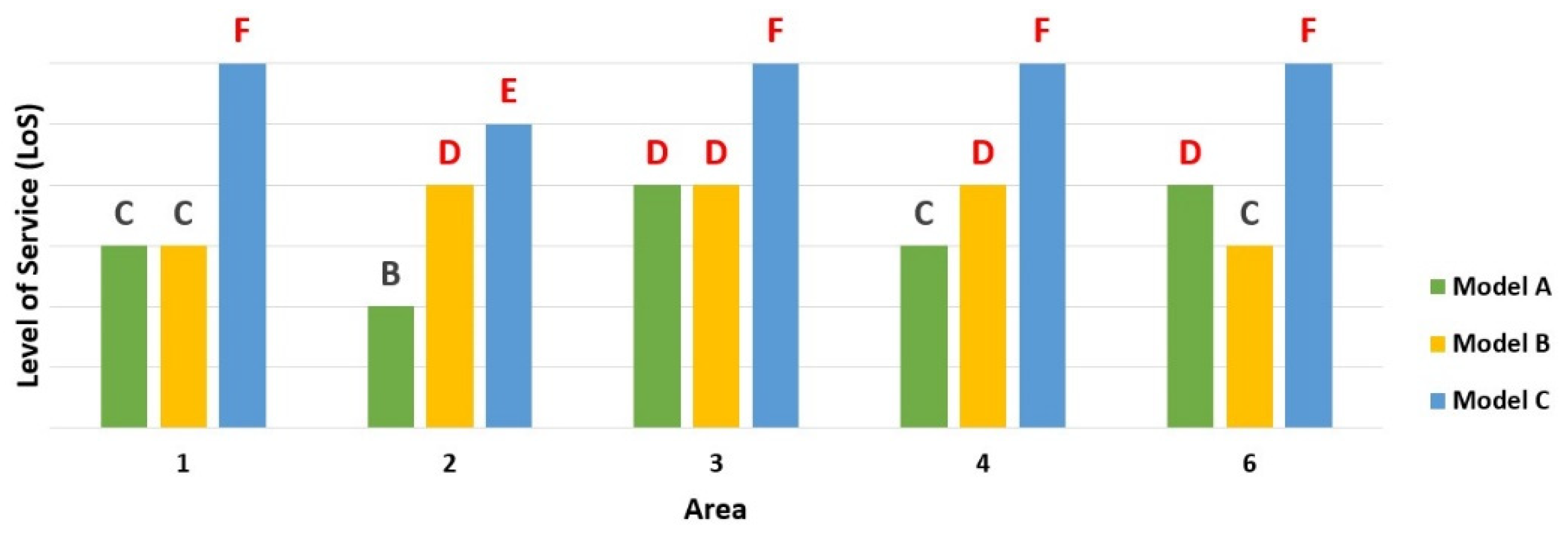
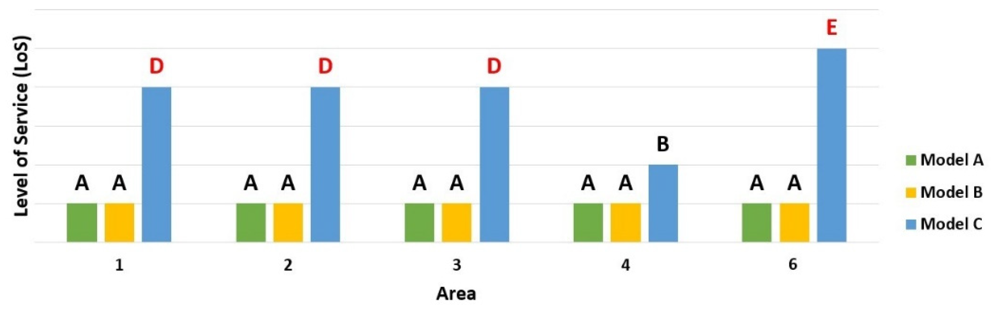
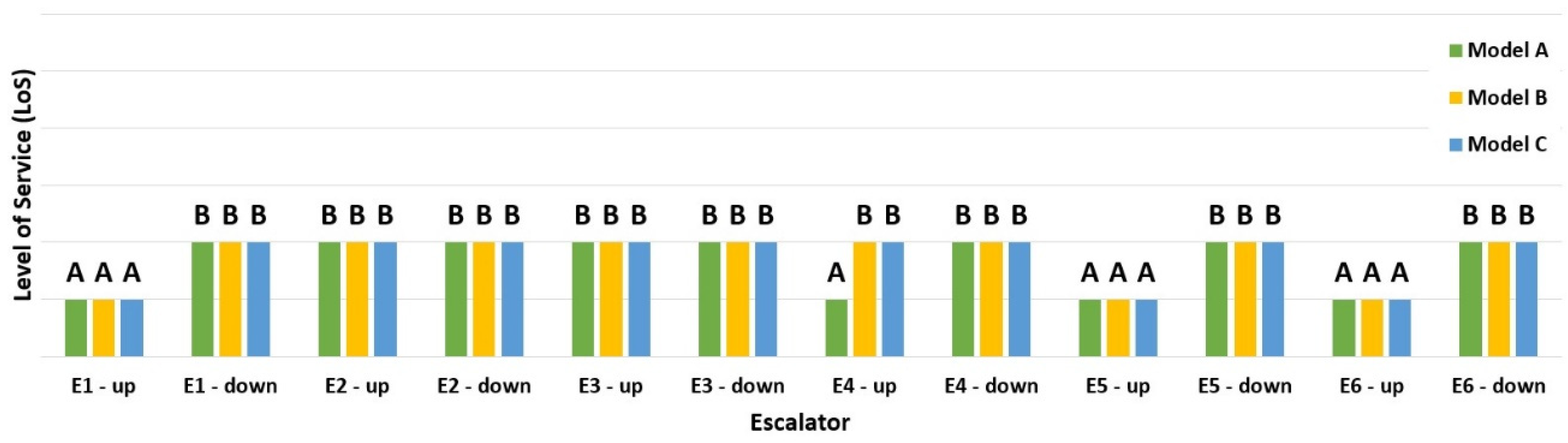
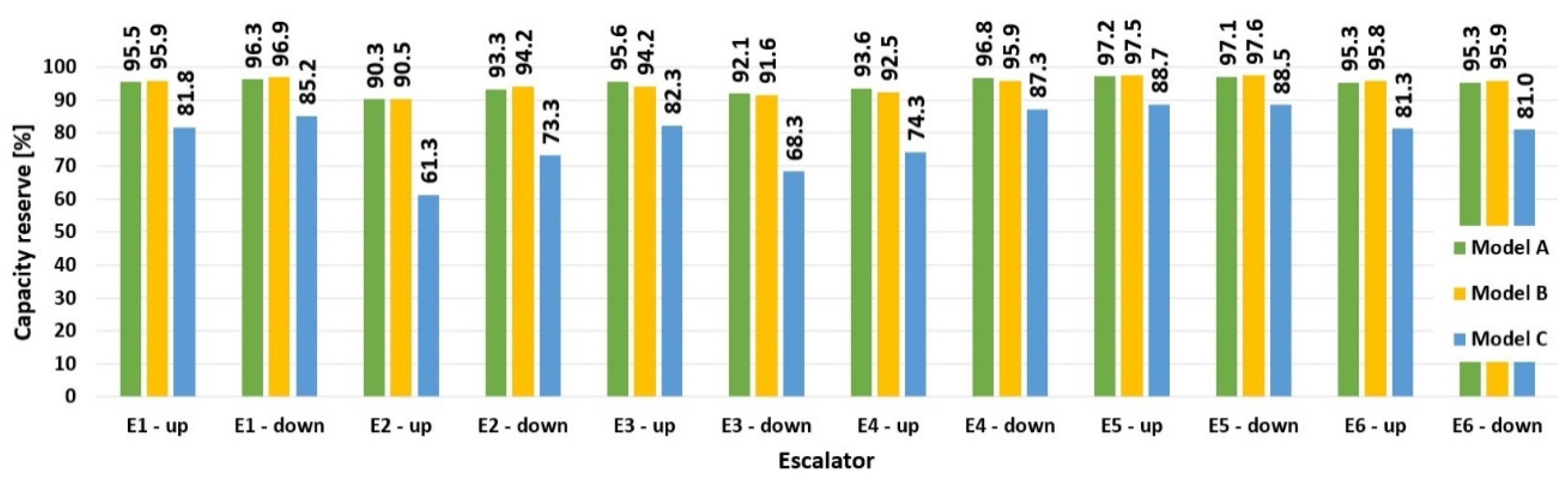
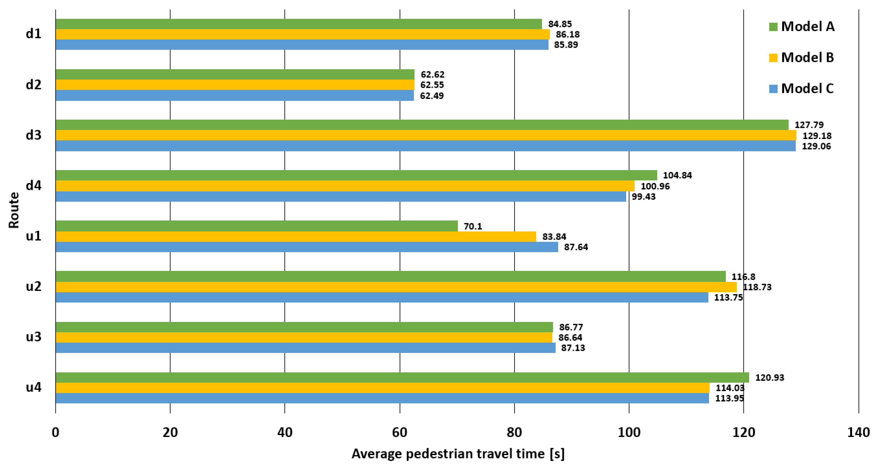
The analyses focused on the evaluation of the Level of Service or on capacity reserves, and various parts of the transit node, i.e., areas intended for movement and waiting (clusters) of passengers, escalators and fixed staircases. Each model was also analysed in terms of travel times of people. From the results given in Section 9 (or see the overall evaluation in Section 9.5), it follows that the analysed transit node is in all observed aspects satisfactory, even in the case of Model C, which is loaded with extraordinary volumes. Certain not excellent results are in case of evaluation of Level of Service for areas used by passengers waiting for a bus/tram connection (especially for Model C), which was expected because in case of extraordinary events, clusters of people at stops are common. In addition, this condition occurs exceptionally.

Although the results presented in the previous sections show that the analysed transit node is suitable in terms of capacity, largely even under extraordinary load, it is always appropriate to think about whether it is realistic, or useful, to increase the capacity (if possible, without significant construction modifications or at high financial costs). If we look, for example, at how the capacity of a standard transport structure can be increased, such as a road or an intersection, it is often the case that additional lanes are added, or these lanes are widened, etc. However, this often leads to disproportionate land use, high financial investments, etc. This trend is certainly not in compliance with transport sustainability, as mentioned in the introduction of this article. In the case of a transit node, in order to increase the capacity of pedestrian areas (either areas for the movement of passengers or areas intended for passengers waiting for a bus/tram connection), or escalators and staircases, their dimension could be increased. However, this is in conflict with what is mentioned earlier, i.e., that there would be expensive construction modifications, which, for example, would not even be possible in the case of the analysed transit node (three-level bridge structure).

It is worth considering increasing the capacity of escalators. Due to their fixed width and the speed of staircases, it can happen that in the case of, for example, a significant jump in pedestrian volumes, the capacity of the escalator will be exceeded. Fortunately for the analysed transit node, the occurrence of this danger is compensated by the fact that there is a standard staircase with sufficient width near each escalator (however, this may not generally be the case). One way to increase the capacity of escalators is to increase their nominal speed. The escalators of the analysed transit node are designed for a nominal speed of 0.5 m/s, and their constructional arrangement does not allow to increase their speed [75]. In the case of a requirement for a higher nominal speed of escalators, the design of the track system, chains, drives, etc., would have to be modified. This would, among other things, result in a change in the dimensions of the escalator design itself (requirement CSN EN 115 [83]). Although this European standard allows solutions with a speed of up to 0.75 m/s (see Table 6), this cannot be applied to the escalators of the analysed transit node, for the reasons stated above. Changing the dimensions of escalators (i.e., changing the length, width and inclination) would again mean financially demanding modifications, which would also not be possible from a construction point of view. For interest, we state here that escalators with a higher nominal speed of 0.75 m/s are used, for example, in the underground of the capital Prague, where, however, there are much higher passenger volumes compared to the transit node we are monitoring. It is also worth considering that higher escalator speeds can cause passengers to keep more distance (for example, for personal safety reasons) and that the actual capacity of the escalator may decrease. People with reduced mobility may also have problems using escalators with higher nominal speeds.

There is also consideration (even commonly practised in some cities) as to whether the capacity of escalators could not be increased by “optically splitting” the escalator into left and right parts (in the direction of movement). In one part, passengers would stand and in the other, faster passengers could “run up/run down” the escalators. However, the experience is that there is a rather negligible increase in the capacity of the escalator. This practice presents problems for escalator operators, as there is more wear on the moving components in the part where the passengers are standing [75], which can cause fault in the escalator and eventually endanger the functionality of the entire transit node. It should be noted that the PTV VISSIM/VISWALK program allows the option of using both sides of the escalators.

On the example of a specific transit node with bus and tram transport, which is built on a bridge construction with three height levels, the use of microsimulation traffic modelling for the capacity evaluation of the transit node was shown. The creation of the model itself is a relatively time-consuming work, which, however, depends on how accurate we want this model, or we need to have. Naturally, the model will never be, and cannot be, an absolutely exact copy of the real world or its parts (here the transit node). It mainly depends on the purpose for which the created model is to be used. The more complicated, or accurate model we require, the more difficult it is to create.

However, subsequent work with the final model (i.e., loading with different volumes of pedestrians and vehicles, making changes in the number of bus/tram connections or links, or changes of the speed of escalators, etc.) brings many significant advantages. These changes can be made relatively quickly in the model (the condition is, of course, to have the appropriate data), and it is also fast to obtain results from the simulations. For example, the PTV VISSIM/VISWALK program performs hourly simulations as standard, which can be “accelerated” when starting this program so that the relevant results are available in about 5 min. This operability is one of the main advantages of microsimulation traffic models, which significantly exceeds the disadvantages associated with long model creation.

The examples given in this article are only a fraction of how the created model of the analysed transit node could be used. A number of other examples of usage could be found, such as using the model to find the optimal solution for timetable changes (which usually occur at the beginning of the year and during the summer holidays) so that the capacity of the transit node is not exceeded and its functionality disrupted. We also see the use of the model at this time influenced by the COVID-19 pandemic, when using the model can well and quickly find optimal solution for the number of connections and sequential arrivals/departures of bus/tram connections to and from stops, so as larger groups of people do not gather together as a part of hygiene measures. The main task of the article was then to point out that the use of microsimulation traffic models can be an important part in the design of transport structures to ensure both the availability of public transport and the required sustainability. Of course, the reality may be different in the end, but the results from the traffic models give us a certain idea of the behaviour of the traffic on the monitored transport structure.

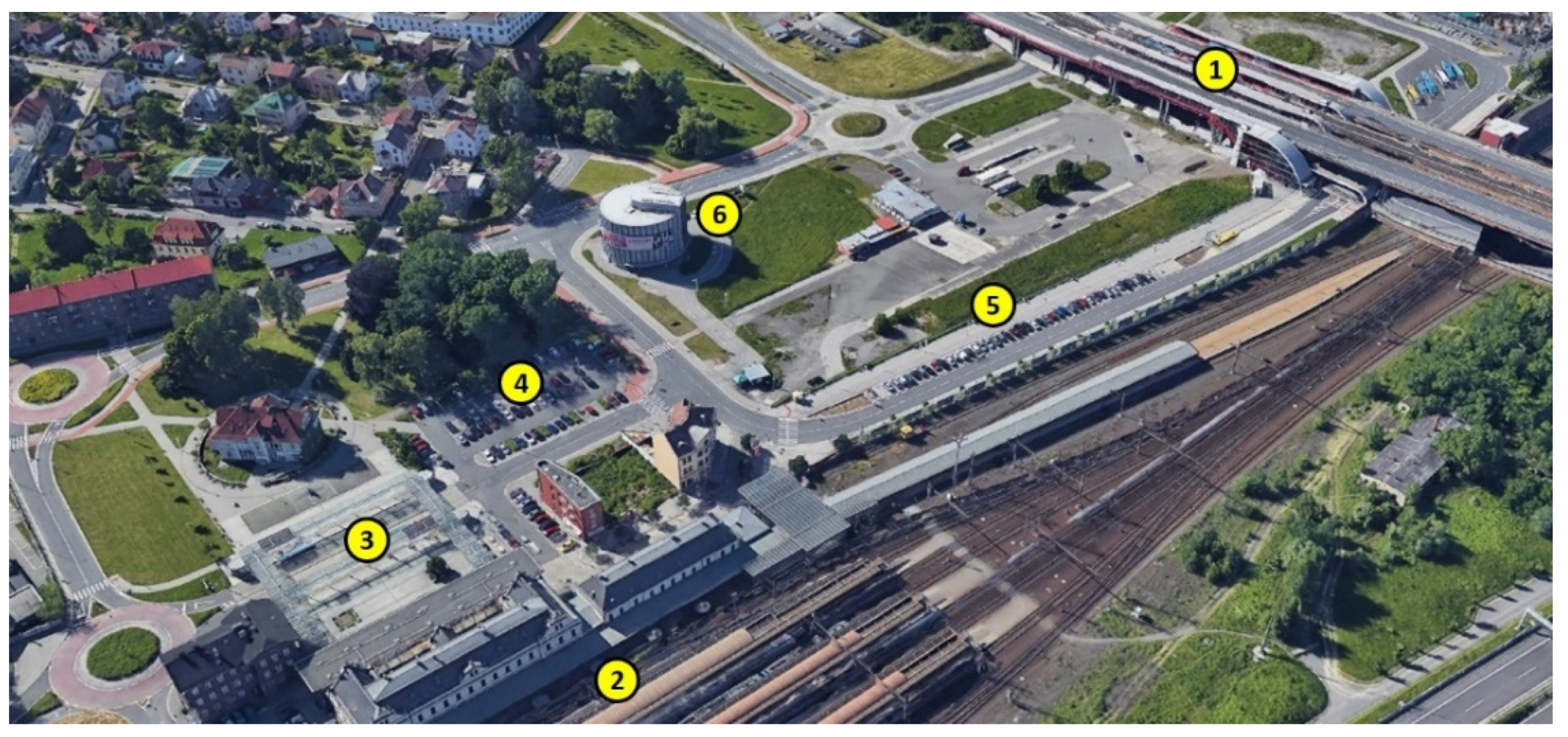
The performed analyses at the transit node are a very important basis for further development of the solved locality. As already mentioned, the location is close to the passenger train station. At present, major changes are planned here in terms of track routing and in the overall modification of the transit node. A high-speed railway is also planned in the locality, which will have a stop at this train station. The overall modification of the railway connection may affect the intensity of pedestrian traffic at the modelled transit node. Furthermore, in the locality between the analysed transit node and the train station, the construction of a three-storey multifunctional building is planned, in which shops, restaurants, etc. will be located. And it will be followed by a 12-storey administrative building. It is obvious that there will be an increase in interest in this locality from the point of view of pedestrians and public transport. Therefore, this model is already properly prepared and tested for future input of relevant data. These requirements were not taken into account in the performed simulations, as the necessary data are currently being collected as part of the construction preparation.

In the Czech Republic, it is not a common practice to use traffic models to simulate the movement of people in such important transport structures. Rather, models related to traffic at intersections, models of evacuation of people, etc., are used. Therefore, the present article dealt with research and the given hypothesis, whether it is possible in our conditions to relevantly use the traffic modelling of the transit node, so that the model is sufficiently effective and ready for further future use.

The presented analysis concerning the capacity evaluation of a chosen transit node using the microsimulation traffic model created in the PTV VISSIM/VISWALK program thus confirms the hypothesis stated in the introduction of this article. Microsimulation traffic models are undoubtedly a suitable tool that can be used in the search for the optimal transport solution of critical points of the public transport network to ensure adequate transport accessibility and related transport sustainability.

References

1. United Nations. Available online: https://sdgs.un.org/goals (accessed on 4 September 2020).
2. Sustainable Development Goals. Available online: https://www.un.org/sustainabledevelopment/sustainable-development-goals/ (accessed on 4 September 2020).
3. Kahle, L.R.; Gurel-Atay, E. Communicating Sustainability for the Green Economy; Routledge, Taylor & Francis Group: London, UK; New York, NY, USA, 2013. [Google Scholar]
4. Krivda, V.; Petru, J.; Macha, D.; Plocova, K.; Fibich, D. An Analysis of Traffic Conflicts as a Tool for Sustainable Road Transport. Sustainability 2020, 12, 7198. [Google Scholar] [CrossRef]
5. James, P.; Magee, L.; Scerri, A.; Steger, M.B. Urban Sustainability in Theory and Practice; Routledge, Taylor & Francis Group: London, UK; New York, NY, USA, 2015. [Google Scholar]
6. Magee, L.; Scerri, A.; James, P.; Thom, J.A.; Padgham, L.; Hickmott, S.; Deng, H.; Cahill, F. Reframing Social Sustainability Reporting: Toward an Engaged. Environ. Dev. Sustain. 2013, 15, 225–243. [Google Scholar] [CrossRef]
7. Krivda, V. Analysis of Conflict Situations in Road Traffic on Roundabouts. Promet Traffic Transp. 2013, 25, 295–303. [Google Scholar] [CrossRef]
8. Martins, V.; Anholon, R.; Quelhas, O. Sustainability Transportation Methods. In Encyclopedia of Sustainability in Hugher Education; Filho, W.L., Ed.; Springer Nature: Basingstoke, UK, 2019; pp. 1–7. [Google Scholar] [CrossRef]
9. Jha, M.K.; Ogallo, H.G.; Owolabi, O. A Quantitative Analysis of Sustainability and Green Transportation Initiatives in Highway Design and Maintenance. Procedia Soc. Behav. Sci. 2014, 111, 1185–1194. [Google Scholar] [CrossRef] [Green Version]
10. Campisi, T.; Canale, A.; Tesoriere, G.; Renčelj, M. The Newest Public Transport System Applied to Turbo Roundabouts. Proc. Inst. Civ. Eng. Eng. Sustain. 2020, 173, 315–322. [Google Scholar] [CrossRef]
11. Petru, J.; Krivda, V. Height and Width Parameters for Ensuring Passage of Excessive Loads on Roads. Acta Polytech. 2017, 57, 209–217. [Google Scholar] [CrossRef]
12. Petru, J.; Krivda, V. The Process of Setting the Parameters for Ensuring Passage of Oversized Cargos. Balt. J. Road Bridg. Eng. 2019, 14, 425–442. [Google Scholar] [CrossRef] [Green Version]
13. Tesoriere, G.; Campisi, T.; Canale, A.; Zgrablic, T. The Surrogate Safety Appraisal of the Unconventional Elliptical and Turbo Roundabouts. J. Adv. Transp. 2018, 2018, 2952074. [Google Scholar] [CrossRef] [Green Version]
14. Ivan, I.; Horak, J.; Zajickova, L.; Burian, J.; Fojtik, D. Factors Influencing Walking Distance to the Preferred Public Transport Stop in Selected Urban Centres of Czechia. GeoScape 2019, 13, 16–30. [Google Scholar] [CrossRef] [Green Version]
15. Campisi, T.; Canale, A.; Tesoriere, G.; Lovric, I.; Cutura, B. The Importance of Assessing the Level of Service in Confined Infrastructures: Some Considerations of the Old Ottoman Pedestrian Bridge of Mostar. Appl. Sci. 2019, 9, 1630. [Google Scholar] [CrossRef] [Green Version]
16. Horak, J.; Tesla, J.; Fojtik, D.; Vozenilek, V. Modelling Public Transport Accessibility with Monte Carlo Stochastic Simulation. Sustainability 2019, 11, 7098. [Google Scholar] [CrossRef] [Green Version]
17. Benenson, I.; Ben-Elia, E.; Rofe, Y.; Geyzersky, D. The Benefits of a High-Resolution Analysis of Transit Accessibility. Int. J. Geogr. Inf. Sci. 2017, 31, 213–236. [Google Scholar] [CrossRef]
18. Tesla, J.; Horak, J.; Ivan, I. Cetnosti spojeni verejnou dopravou mezi obcemi v krajich Ceske republiky (in Czech). Perners Contacts 2015, 10, 176–184. [Google Scholar]
19. Wolek, M.; Wolanski, M.; Bartlomiejczyk, M.; Wyszomirssi, O.; Grzles, K.; Hebel, K. Ensuring Sustainable Development of Urban Public Transport: A case Study of the Trolleybus System in Gdynia and Sopot (Poland). J. Clean. Prod. 2020, 279, 123807. [Google Scholar] [CrossRef]
20. Fu, X.; Qiang, Y.; Wang, J.; Zhao, X.; Hwang, F.J.; Chen, C.H. Urban Public Transport Accessibility to Medical Service from the Perspective of Residents’ Travel: A Hybrid Assessment Based on the Whole Process. IEEE Access 2021, 9, 8977–8989. [Google Scholar] [CrossRef]
21. Bentlage, M.; Muller, C.; Thierstein, A. Becoming More Polycentric: Public Transport and Location Choices in the Munich Metropolitan Area. Urban Geogr. 2020. [Google Scholar] [CrossRef]
22. Liu, Y.; Cheng, T. Understanding Public Transit Patterns with Open Geodemographics to Facilitate Public Transport Planning. Transp. A Transp. Sci. 2020, 16, 76–103. [Google Scholar] [CrossRef] [Green Version]
23. Heyken Soares, P.; Ahmed, L.; Mao, Y.; Mumford, C.L. Public Transport Network Optimisation in PTV Visum Using Selection Hyper-Heuristics. Public Transp. 2020. [Google Scholar] [CrossRef]
24. Wang, W.; Wang, Y.; Homem de Almeida Correia, G.; Chen, Y. A Network-Based Model of Passenger Transfer Flow between Bus and Metro: An Application to the Public Transport System of Beijing. J. Adv. Transp. 2020, 2020, 6659931. [Google Scholar] [CrossRef]
25. Gnecco, G.; Hadas, Y.; Sanguineti, M. Public Transport Transfers Assessment via Transferable Utility Games and Shapley Value Approximation. Transp. A Transp. Sci. 2020. [Google Scholar] [CrossRef]
26. Naumov, V.; Samchuk, G. Class Library for Simulation of Passenger Transfer Nodes as Elements of the Public Transport System. In Proceedings of the 10th International Scientific Conference Transbaltica 2017: Transportation Science and Technology, Vilnius, Lithuania, 4–5 May 2017. [Google Scholar] [CrossRef]
27. Schakenbos, R.; Paix, L.L.; Nijenstein, S.; Geurs, K.T. Valuation of a Transfer in a Multimodal Public Transport Trip. Transp. Policy 2016, 46, 72–81. [Google Scholar] [CrossRef]
28. Michel, S.; Chidlovskii, B. Stochastic Optimization of Public Transport Schedules to Reduce Transfer Waiting Times. In Proceedings of the IEEEE International Smart Cities Conference (ISC2), Trento, Italy, 12–15 September 2016. [Google Scholar] [CrossRef]
29. Chen, Q.; Zheng, N.; Bai, Y. Simulation and Optimization of Pedestrian Regular Evacuation in Comprehensive Rail Transit Hub—A Case Study in Beijing. Promet Traffic Transp. 2020, 32, 383–397. [Google Scholar] [CrossRef]
30. Drliciak, M.; Celko, J.; Cingel, M.; Jandacka, D. Traffic Volumes as a Modal Split Parameter. Sustainability 2020, 12, 10252. [Google Scholar] [CrossRef]
31. Drliciak, M.; Celko, J. Implementation of Transport Data in to the Transport Forecasting in Slovakia. In Proceedings of the 6th Transport Research Arena (TRA), Warsaw, Poland, 18–21 April 2016. [Google Scholar] [CrossRef] [Green Version]
32. Arliansyah, J.; Praseyo, M.R.; Kurnia, A.Y. Planning of City Transportation Infrastructure Based on Macro Simulation Model. Int. J. Adv. Sci. Eng. Inf. Technol. 2017, 7, 1262–1267. [Google Scholar] [CrossRef] [Green Version]
33. Tiessler, M.; Engelhardt, R.; Bogenberger, K.; Hessel, C. Integration of an Urban Ropeway into Munich´s Transit System Demand Modeling. Transp. Res. Rec. 2019, 2673, 47–57. [Google Scholar] [CrossRef]
34. Jacyna, M.; Wasiak, M.; Klodawski, M.; Golebiowski, P. Modelling of Bicycle Traffic in the Cities Using VISUM. In Proceedings of the 10th International Scientific Conference Transbaltica 2017: Transportation Science and Technology, Vilnius, Lithuania, 4–5 May 2017. [Google Scholar] [CrossRef]
35. Myronenko, S.V.; Gillis, D. Modelling of Road Traffic for Traffic Flow Optimization of Modern Regional Center as an Example of Odessa, Ukraine. Comput. Inf. Netw. Syst. 2016, 3, 54–64. [Google Scholar] [CrossRef]
36. Kotsialos, A.; Papageorgiou, M.; Diakaki, C.; Pavlis, Y.; Middelham, F. Traffic Flow Modeling of Large-Scale Motorway Networks Using the Macroscopic Modeling Tool METANET. IEEE Trans. Intell. Transp. Syst. 2002, 3, 282–292. [Google Scholar] [CrossRef] [Green Version]
37. Cernicky, L.; Kalsova, A.; Kapusta, J. Signal Controlled Junctions Calculations in Traffic-Capacity Assessment—Aimsun, OmniTrans, Webster and TP 10/2010 Results Comparison. Transp. Probl. 2016, 11, 121–130. [Google Scholar] [CrossRef] [Green Version]
38. Cernicky, L.; Kalsova, A.; Mikulski, J. Simulation Software as a Calculation Tool for Traffic Capacity Assessment. Commun. Sci. Lett. Univ. Zilina 2016, 18, 99–103. [Google Scholar]
39. Jagersma, M.; Reid, C.; Potesil, T. Application of Streamline in Australian Cities. In Proceedings of the 37th Australasian Transport Research Forum (ATRF 2015), Sydney, Australia, 30 September–2 October 2015. [Google Scholar]
40. Tollazzi, T.; Lerher, T.; Sraml, M. The Use of Micro-Simulation in Determining the Capacity of a Roundabout with a Multi-Channel Pedestrian Flow. Stroj. Vestn. J. Mech. Eng. 2008, 54, 334–346. [Google Scholar]
41. Istoka Otkovic, I.; Tollazzi, T.; Sraml, M. Calibration of Microsimulation Traffic Model Using Neural Network Approach. Expert Syst. Appl. 2013, 40, 5965–5974. [Google Scholar] [CrossRef]
42. Otkovic, I.I.; Deluka-Tibljas, A.; Surdonja, S. Validation of the Calibration Methodology of the Micro-Simulation Traffic Model. Transp. Res. Procedia 2020, 45, 684–691. [Google Scholar] [CrossRef]
43. Gipps, P.G. A Model for the Structure of Lane-Changing Decisions. Transp. Res. Part B Methodol. 1986, 20, 403–414. [Google Scholar] [CrossRef]
44. Sparmann, U. Spurwechselvorgange auf Zweispurigen BAB-Richtungsfahrbahnen. Ph.D. Thesis, Universitat Karlsruhe, Karlsruhe, Germany, 1978. [Google Scholar]
45. Zhang, Y. Scalability of Car-Following and Lane-Changing Models in Microscopic Traffic Simulation Systems. Master’s Thesis, Louisiana State University, Baton Rouge, LA, USA, 2004. [Google Scholar]
46. Fyfe, M.R.W. Safety Evaluation of Connected Vehicle Applications Using Micro-Simulation. Master’s Thesis, University of British Columbia, Vancouver, BC, Canada, 2016. [Google Scholar]
47. Stromgren, P.; Olstam, J.; Tapani, A. A Model for Traffic Simulation of Flared Rural Road Intersections. Transp. Res. Procedia 2015, 6, 239–258. [Google Scholar] [CrossRef] [Green Version]
48. Mohammadi, A.; Chowdhury, M.T.U.; Yang, S.; Park, P.Y. Developing Levels of Pedestrian Physical Distancing during a Pandemic. Saf. Sci. 2021, 134, 105066. [Google Scholar] [CrossRef]
49. Barcelo, J.; Codina, E.; Casas, J.; Ferrer, J.L.; Garcia, D. Microscopic Traffic Simulation: A Tool for the Design analysis and Evaluation of Intelligent Transport Systems. J. Intell. Robot. Syst. 2005, 41, 173–203. [Google Scholar] [CrossRef]
50. Barcelo, J.; Casas, J. Dynamic Network Simulation with AIMSUN. In Simulation Approaches in Transportation Analysis; Springer: Berlin/Heidelberg, Germany, 2005; pp. 57–98. [Google Scholar] [CrossRef]
51. Lu, X.-Y.; Qiu, T.Z.; Varaiya, P.; Horowitz, R.; Shladover, S.E. Combining Variable Speed Limits with Ramp Metering for Freeway Traffic Control. In Proceedings of the American Control Conference, Baltimore, MD, USA, 30 June–2 July 2010; pp. 2266–2271. [Google Scholar] [CrossRef]
52. Jones, S.L.; Sullivan, A.J.; Cheekoti, N.; Anderson, M.D.; Malave, D. Traffic Simulation Software Comparison Study; University of Alabama: Tuscaloosa, AL, USA, 2004. [Google Scholar]
53. Olia, A.; Genders, W.; Razavi, S.N. Microsimulation-Based Impact Assessment of the Vehicle-to-Vehicle (V2V) System for Work Zone Safety. In Proceedings of the CSCE 2013 General Conference (Congres General 2013 de la SCGC), Montreal, QC, Canada, 29 May–1 June 2013. [Google Scholar]
54. Olstam, J.J.; Tapani, A. Comparison of Car-Following Models; Swedish National Road and Transport Research Institute: Linköping, Sweden, 2004. [Google Scholar]
55. Fritzsche, H.T. A Model for Traffic Simulation. Traffic Eng. Control 1994, 35, 317–321. [Google Scholar]
56. Waizman, G.; Shoval, S.; Benenson, I. Traffic Accident Risk Assessment with Dynamic Microsimulation Model Using Range-Range Rate Graphs. Accid. Anal. Prev. 2018, 119, 248–262. [Google Scholar] [CrossRef] [PubMed]
57. Van Arem, B.; Tampere, C.M.J.; Malone, K.M. Modelling Traffic Flows with Intelligent Cars and Intelligent Roads. In Proceedings of the IEEE IV 2003 Intelligent Vehicles Symposium, Columbus, OH, USA, 9–11 June 2003; pp. 456–461. [Google Scholar] [CrossRef]
58. Van Arem, B.; Van Driel, C.J.G.; Visser, R. The Impact of Cooperative Adaptive Cruise Control on Traffic-Flow Characteristics. IEEE Trans. Intell. Transp. Syst. 2007, 7, 429–436. [Google Scholar] [CrossRef] [Green Version]
59. Lochrane, T.W.P. A New Multidimensional Psycho-Physical Framework for Modeling Car-Following in a Freeway Work Zone. Ph.D. Thesis, University of Central Florida, Orlando, FL, USA, 2014. [Google Scholar]
60. Soria, I.; Elefteriadou, L.; Kondyli, A. Assessment of Car-Following Models by Driver Type and Under Different Traffic, Weather Conditions Using Data from an Instrumented Vehicle. Simul. Model. Pract. Theory 2014, 40, 208–220. [Google Scholar] [CrossRef]
61. Brackstone, M.; McDonald, M. Car-Following: A Historical Review. Transp. Res. Part F Traffic Psychol. Behav. 1999, 2, 181–196. [Google Scholar] [CrossRef]
62. Pipes, L.A. An Operational Analysis of Traffic Dynamics. J. Appl. Phys. 1953, 24, 274–281. [Google Scholar] [CrossRef]
63. PTV Group. PTV Vissim 2020 User Manual; PTV Group: Karlsruhe, Germany, 2020. [Google Scholar]
64. Wiedemann, R. Simulation des Verkehrsflusses; Schriftenreihe des Instituts für Verkehrswesen, Universität Karlsruhe: Karlsruhe, Germany, 1974; p. 84. [Google Scholar]
65. Wiedemann, R.; Reiter, U. Microscopic Traffic Simulation: The Simulation System MISSION, Background and Actual State; Project ICARUS (V1052) Final Report; CEC: Brussels, Belgium, 1992; pp. 1–53. [Google Scholar]
66. Helbing, D.; Johansson, A. Pedestrian, Crowd and Evacuation Dynamics. In Encyclopedia of Complexity and System Science; Meyers, R.A., Ed.; Springer: Berlin/Heidelberg, Germany; New York, NY, USA, 2009; Volume 16, pp. 6476–6495. [Google Scholar]
67. Helbing, D.; Molnar, P. Social Force Model for Pedestrian Dynamics. Phys. Rev. E 1995, 51, 4282–4286. [Google Scholar] [CrossRef] [PubMed] [Green Version]
68. Helbing, D.; Farkas, I.J.; Vicsek, T. Simulating Dynamic Features of Escape Panic. Nature 2000, 407, 487–490. [Google Scholar] [CrossRef] [PubMed] [Green Version]
69. Helbing, D.; Farkas, I.J.; Molnar, P.; Vicsek, T. Simulation of Pedestrian Crowd in Normal and Evacuation Situations. In Pedestrian and Evacuation Dynamics; Schreckenberg, M., Sharma, S.D., Eds.; Springer: Berlin/Heidelberg, Germany, 2001; pp. 21–58. [Google Scholar]
70. Lovas, G.G. Modeling and Simulation of Pedestrian Traffic Flow. Transp. Res. Part B Methodol. 1994, 28, 429–443. [Google Scholar] [CrossRef]
71. Liu, M.; Zeng, W.; Chen, P.; Wu, X. A Microscopic Simulation Model for Pedestrian-Pedestrian and Pedestrian-Vehicle Interactions at Crosswalks. PLoS ONE 2017, 12, 1–23. [Google Scholar] [CrossRef] [Green Version]
72. Blue, V.J.; Adler, J.L. Cellular Automata Microsimulation of Bidirectional Pedestrian Flows. Transp. Res. Rec. 1999, 1678, 135–141. [Google Scholar] [CrossRef]
73. Blue, V.J.; Adler, J.L. Emergent Fundamental Pedestrian Flows from Cellular Automata Microsimulation. Transp. Res. Rec. 1998, 1644, 29–36. [Google Scholar] [CrossRef]
74. Hoogendoorn, S.P.; Bovy, P.H.L.; Daamen, W. Microscopic Pedestrian Wayfinding and Dynamics Modelling. In Pedestrian and Evacuation Dynamics; Schreckenberg, M., Sharma, S.D., Eds.; Springer: Berlin/Heidelberg, Germany, 2001; pp. 123–154. [Google Scholar]
75. Daskova, H. Capacity Assessment of Transit Node by Micro Simulation Model. Ph.D. Thesis, VSB—Technical University of Ostrava, Ostrava, Czech Republic, 1 December 2017. [Google Scholar]
76. Banks, J. (Ed.) Handbook of Simulation: Principles, Methodology, Advances, Applications, and Practice; John Wiley & Sons: Hoboken, NJ, USA, 1998; pp. 15–18. [Google Scholar]
77. Rezac, M.; Tichy, J.; Skvain, V. Dopravni Inzenyrstvi; VSB—Technical University of Ostrava: Ostrava, Czech Republic, 2010; pp. 155–160. (In Czech) [Google Scholar]
78. Google Earth. Available online: https://eart.google.com (accessed on 4 October 2020).
79. Scheme of Transit Node Ostrava-Svinov. Available online: https://www.kodis.cz./pdf/Ostrava_Svinov.pdf (accessed on 4 October 2020).
80. Planned Routes Extension of Tram Transport in Ostrava-Poruba. Available online: https://novatramvajporuba.cz/trasy (accessed on 10 October 2020).
81. Ostrava Public Transport. Available online: www.dpo.cz (accessed on 1 October 2020).
82. CSN 73 6110 Design of Urban Roads; Czech Technical Standard; Czech Office for Standards, Metrology and Testing: Prague, Czech Republic, 2006.
83. CSN EN 115 Safety of Escalators and Moving Walkways; Czech Technical Standard; Czech Office for Standards, Metrology and Testing: Prague, Czech Republic, 2019.
84. Svinov-Mosty: Project Documentation; Dopravoprojekt: Ostrava, Czech Republic, 2012.
Figure 1. Description of the analysis of traffic problem using the simulation model.
Sustainability 13 02709 g001
Figure 2. Analysed transit node (1) and its surroundings ((2)—train station, (3)—urban and long-distance bus stops, (4) + (5)—car park, and (6)—parking house) [78].
Sustainability 13 02709 g002
Figure 3. The analysed transit node and its parts ((1)—bus stop on the 2nd floor, (2)—view from the bus stop to the tram stop on the 2nd floor, (3)—the north staircase tower, (4)—turning bay of buses, (5)—connecting corridor on the 1st floor, (6)—bus stops on the ground floor, (7)—escalators in the south staircase tower, (8)—view on the escalators and the access to the lift on the 2nd floor, and (9)—internal staircase towers) [75,78].
Sustainability 13 02709 g003
Figure 4. A diagram of the analysed transit node ((1)—the north staircase tower, (2)—internal staircase towers, (3)—the south staircase tower, (4)—lifts (L1–L4), (5)—ticket machines, (6)—escalators (E1–E6), (7)—staircase (S1–S7), T1 + T2—tram stops on the 2nd floor, H1–H8—bus stops on the 2nd floor, D1 + D2—bus stops on the ground floor). Modified from [79].
Sustainability 13 02709 g004
Figure 5. A diagram of tram and bus links marking the new tram line, where (1)—the analysed transit node, (2)—the new tram line (green colour, A + B—beginning/end of the new tram line), 49—cancelled part of bus link no. 49 (yellow dashed line), red—existing tram links, blue—existing bus urban links, and purple—existing long-distance bus links. Modified from [79,81].
Sustainability 13 02709 g005
Figure 6. Determination of the size of pedestrian areas (1 + 2—bus platforms on the 2nd floor, 3 + 4—tram platforms on the 2nd floor, 5—connecting corridor on the 1st floor, 6—space for pedestrians on the ground floor). Modified from [75,79].
Sustainability 13 02709 g006
Figure 7. A drawing of the analysed transit node, which was used as a plan view basis for the traffic model ((a)—overall situation, and (b)—detail of the stairs, escalators, etc.) [75,84].
Sustainability 13 02709 g007
Figure 8. An example of a microsimulation traffic model of the analysed transit node in the PTV VISSIM/VISWALK program in 2D ((a)—full view, and (b)—simplified view, the so-called toggle wireframe).
Sustainability 13 02709 g008
Figure 9. An example of a microsimulation traffic model of the analysed transit node in the PTV VISSIM/VISWALK program in 3D.
Sustainability 13 02709 g009
Figure 10. An example of the movement (yellow lines) of individual pedestrian flows (a) and an example of chosen attributes (b), i.e., the name of the route, volumes, etc. in a microsimulation model created in the PTV VISSIM/VISWALK program.
Sustainability 13 02709 g010
Figure 11. An example of running simulation in a microsimulation model created in the PTV VISSIM/VISWALK program ((AE)—individual detailed views of chosen parts of the model).
Sustainability 13 02709 g011
Figure 12. Dependence of density of pedestrians on monitored pedestrian areas in time for Model A (afternoon peak hour from 3 p.m. to 4 p.m.; 1–6—designation of pedestrian areas according to Figure 6).
Sustainability 13 02709 g012
Figure 13. Dependence of density of pedestrians on the observed pedestrian areas in time for Model B (afternoon peak hour from 3 p.m. to 4 p.m.; 1–6—designation of pedestrian areas according to Figure 6).
Sustainability 13 02709 g013
Figure 14. Dependence of density of pedestrians on the observed pedestrian areas in time for Model C (afternoon peak hour from 3 p.m. to 4 p.m.; 1–6—designation of pedestrian areas according to Figure 6).
Sustainability 13 02709 g014
Figure 15. Level of Service for pedestrians in the cluster in peak hour for Models A, B and C (area nos. 1–4 and 6; see Figure 6).
Sustainability 13 02709 g015
Figure 16. Level of Service for pedestrians in the cluster for a 15 min peak for Models A, B and C (area nos. 1–4 and 6; see Figure 6).
Sustainability 13 02709 g016
Figure 17. Level of Service of escalators for Models A, B and C (for designation of escalators E1–E6, see Figure 7).
Sustainability 13 02709 g017
Figure 18. Capacity reserve of escalators for Models A, B and C (for designation of escalators E1–E6, see Figure 7).
Sustainability 13 02709 g018
Figure 19. Overall evaluation of chosen travel times for pedestrians for Models A, B and C (afternoon peak hour from 3 p.m. to 4 p.m.; d1–d4 and u1–u4, see Section 9.1.4 or Table 13, Table 20 and Table 27).
Sustainability 13 02709 g019