
The Predictive Capability of a Novel Ensemble Tree-Based Algorithm for Assessing Groundwater Potential


Abstract
1. Introduction
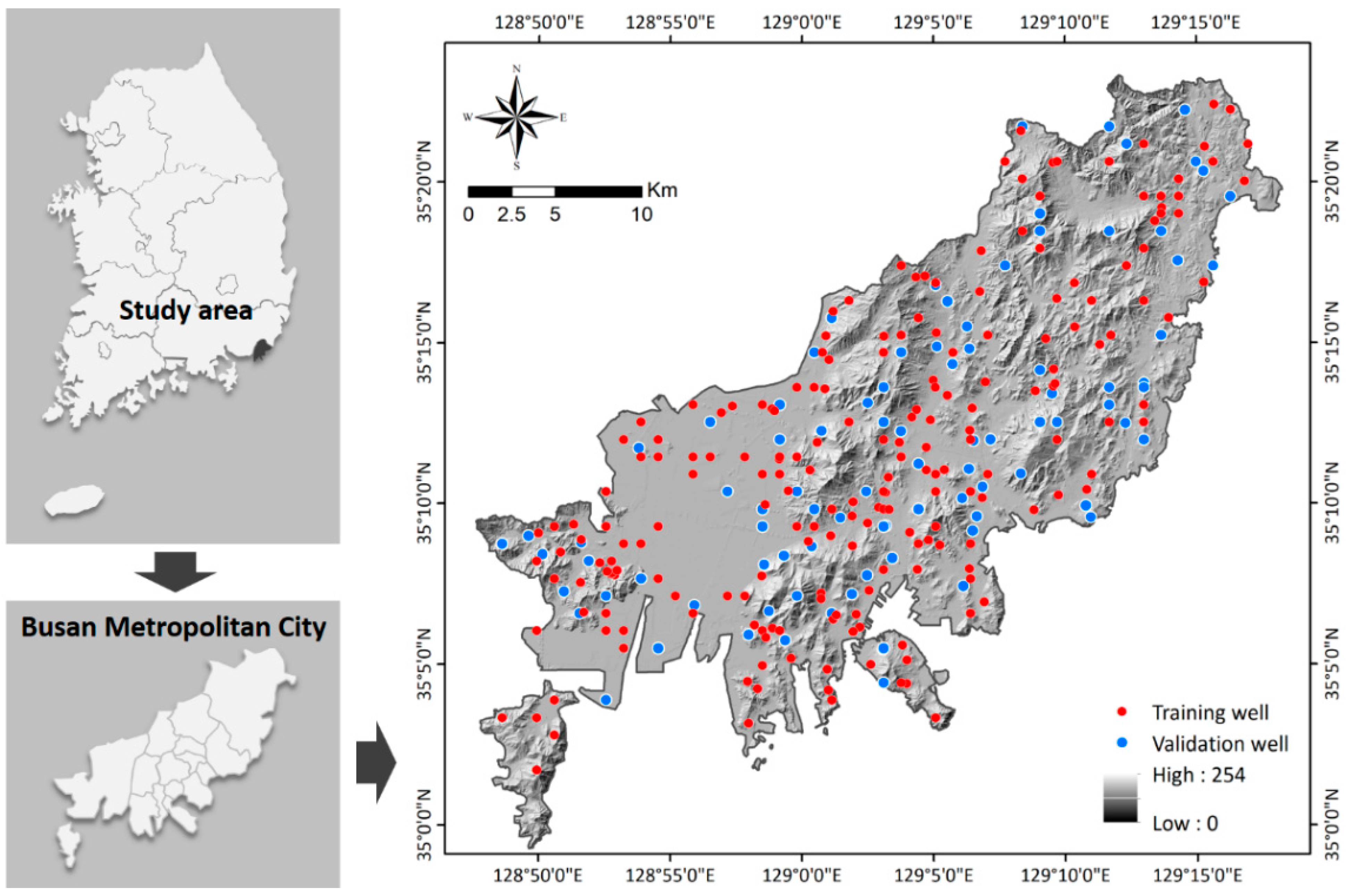
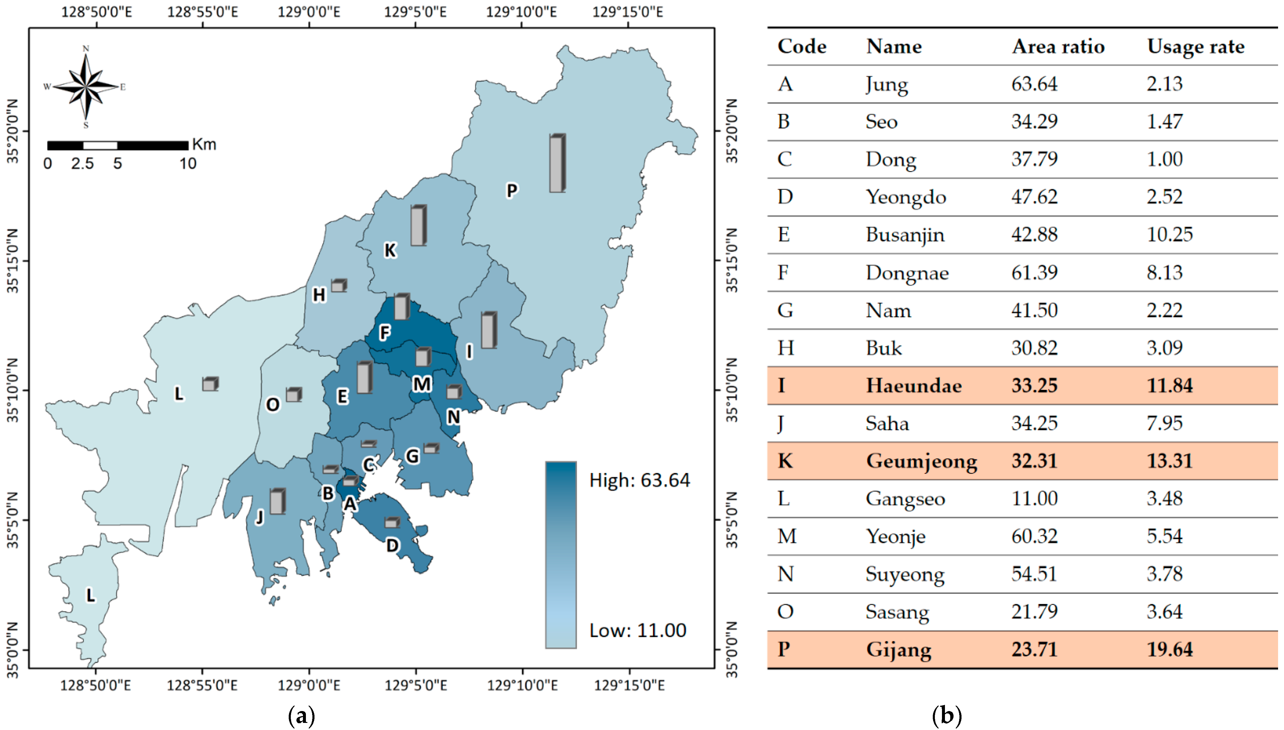
2. Study Area
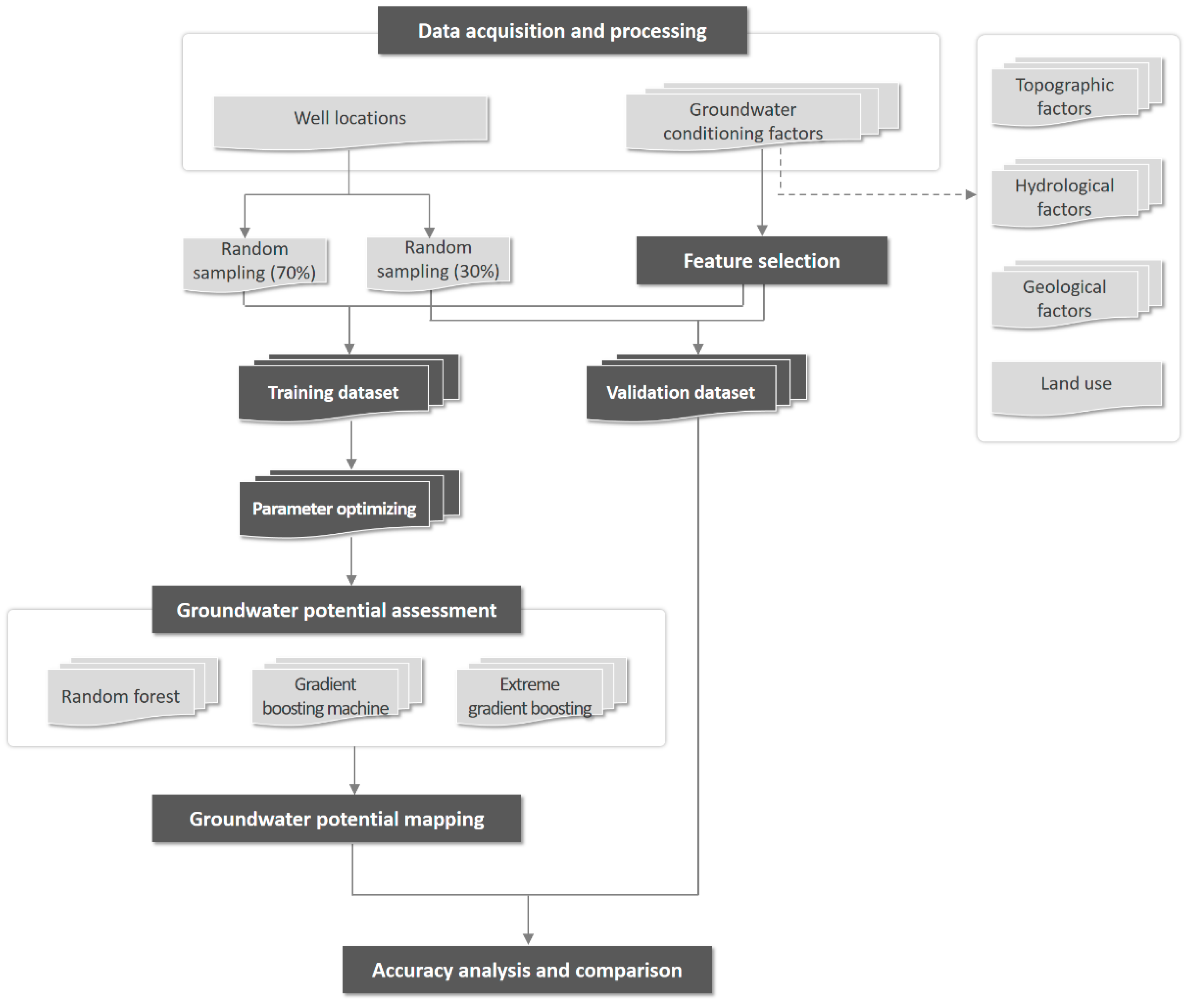
3. Materials and Methods
3.1. Construction of the Spatial Database
3.1.1. Well Data
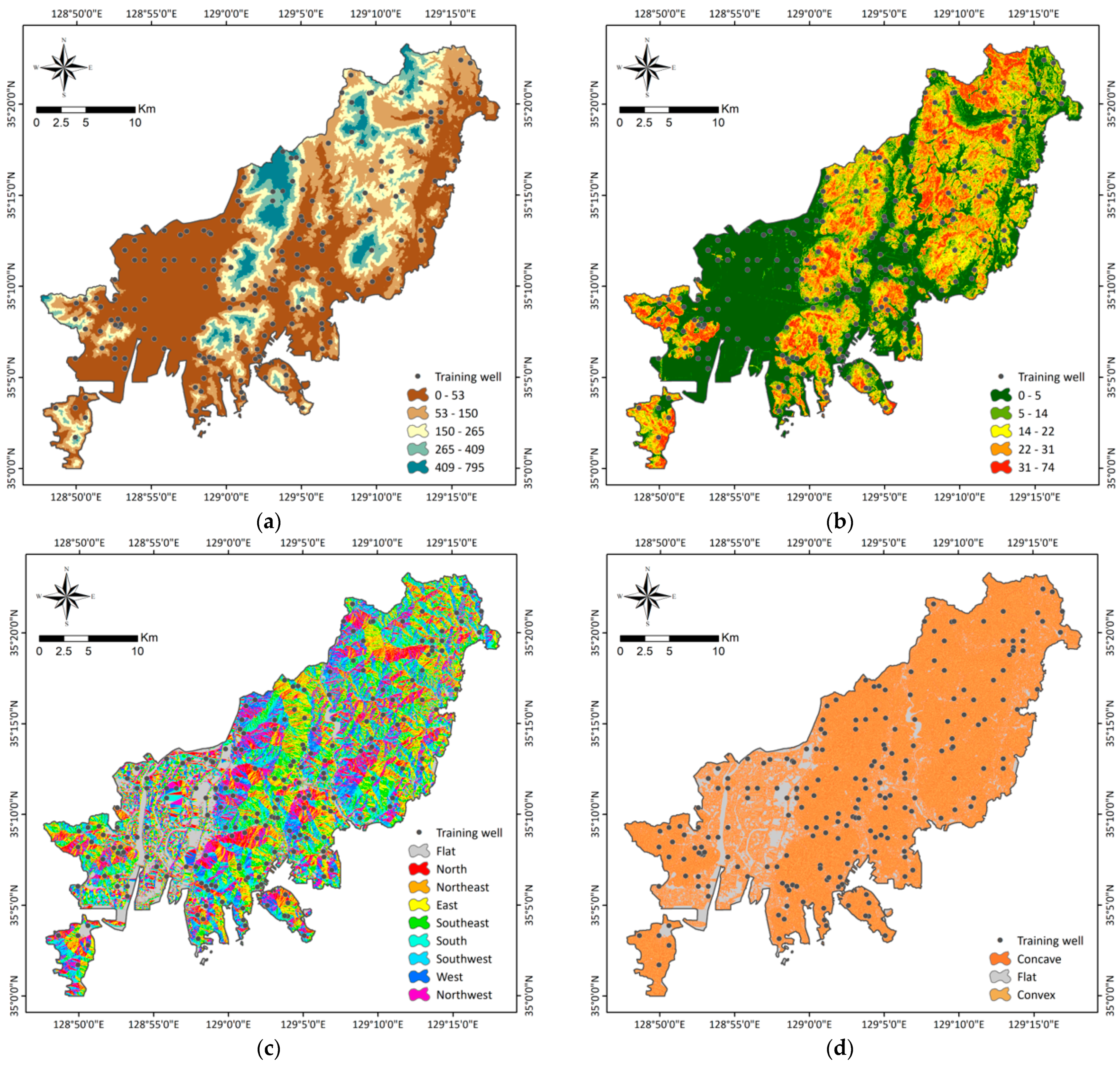
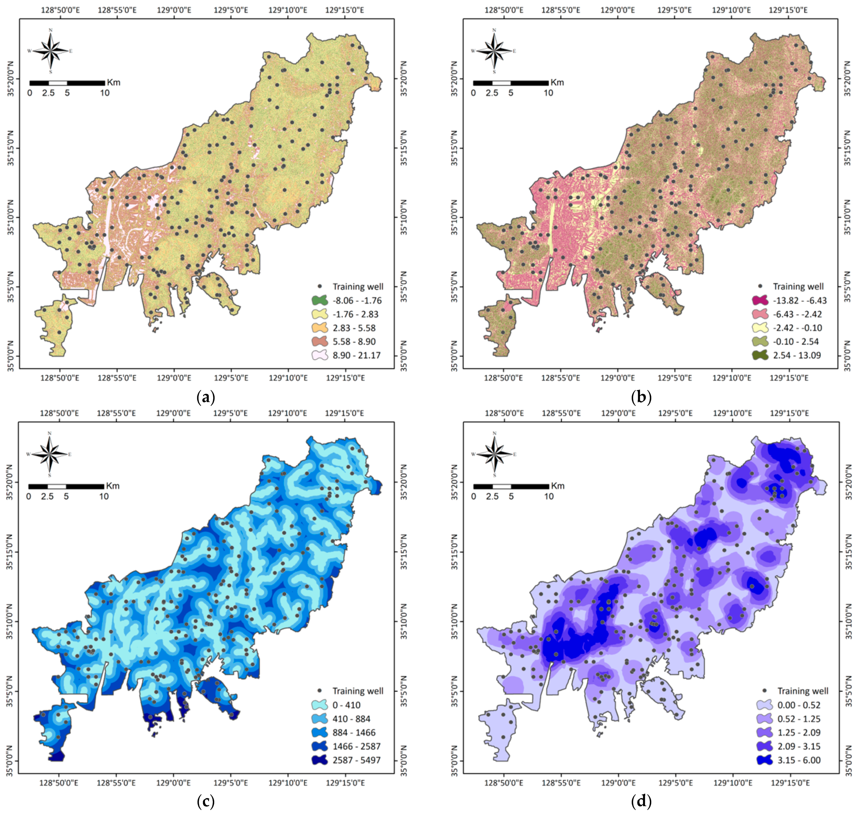
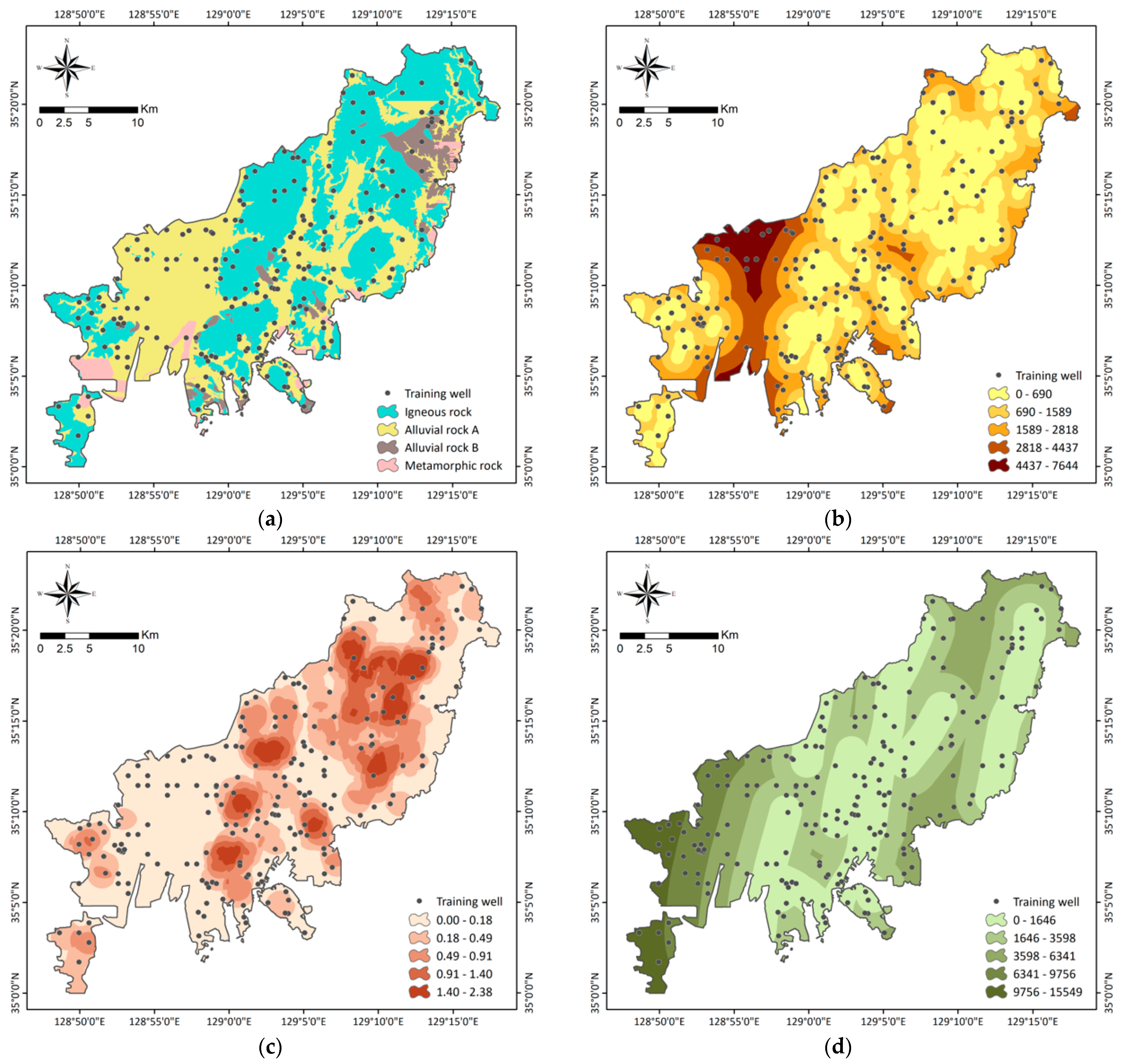
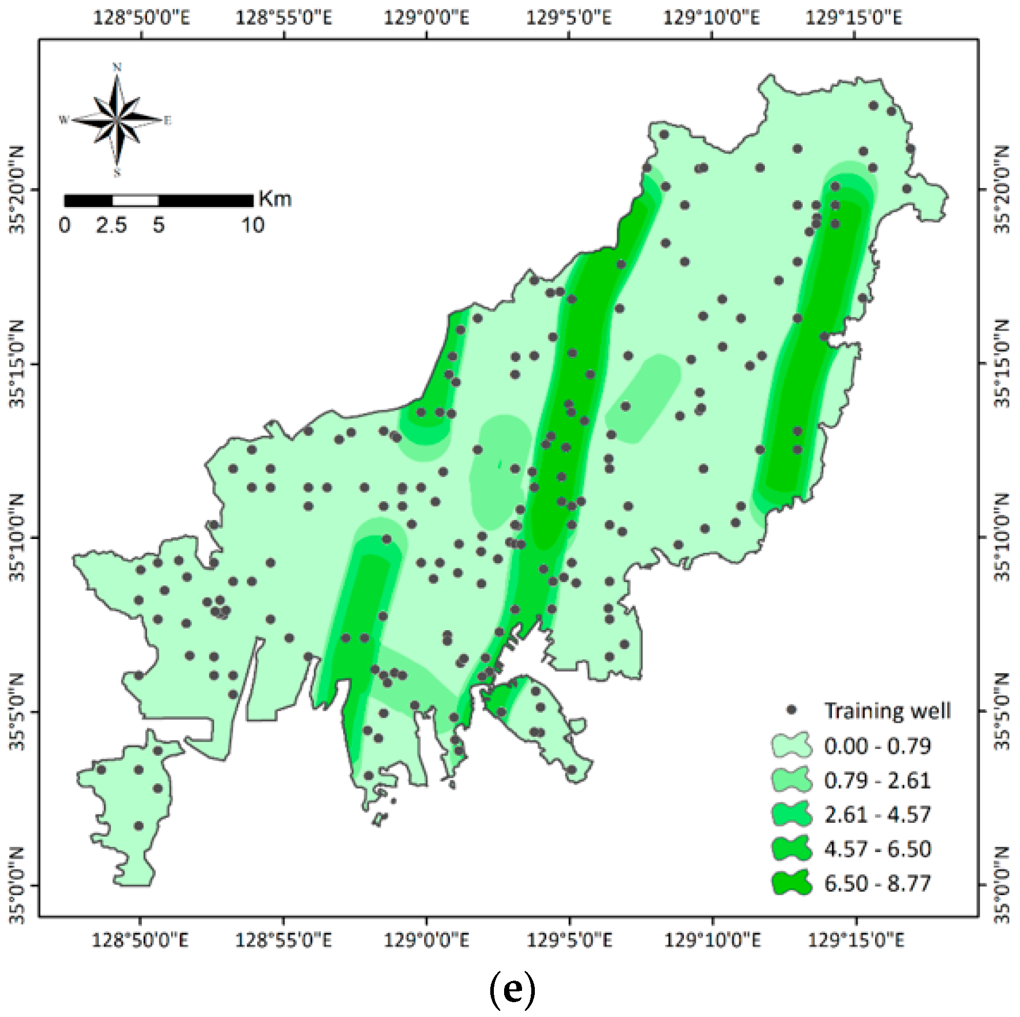
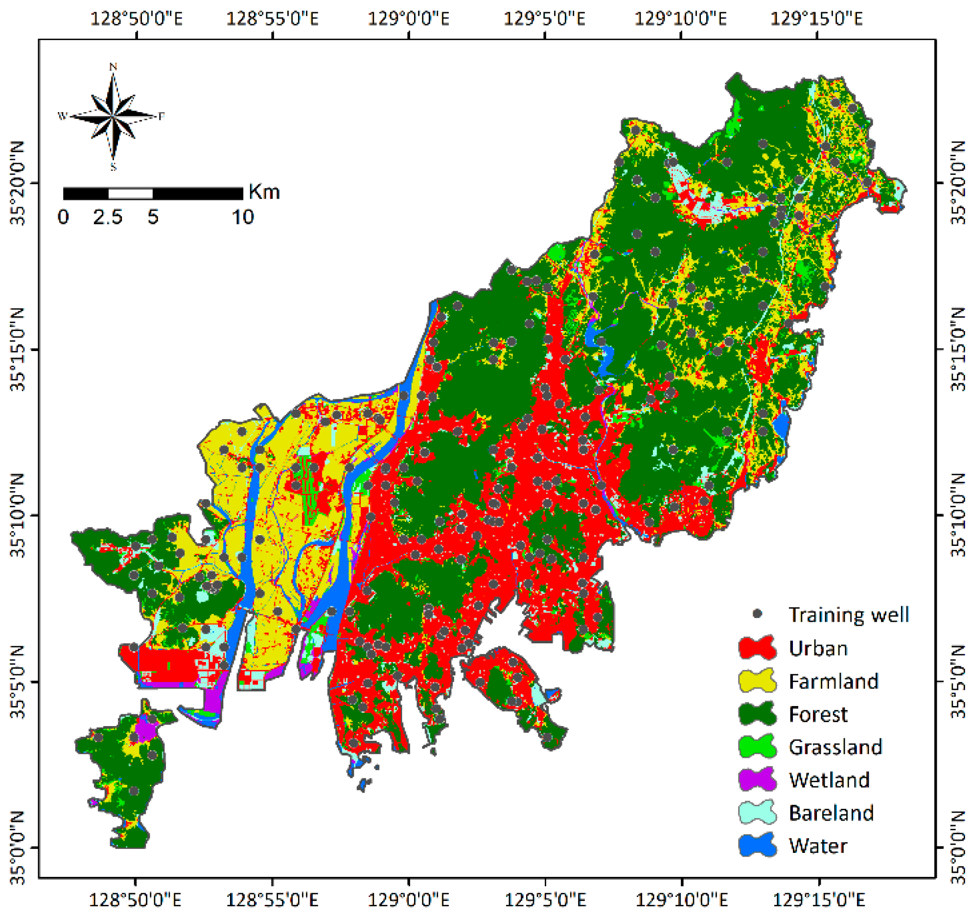
3.1.2. Groundwater Conditioning Factors
3.2. Selection of Groundwater Conditioning Factors
3.3. Groundwater Potential Modeling
3.3.1. Random Forest
3.3.2. Gradient Boost Machine
3.3.3. Extreme Gradient Boosting
4. Results
4.1. Feature Selection
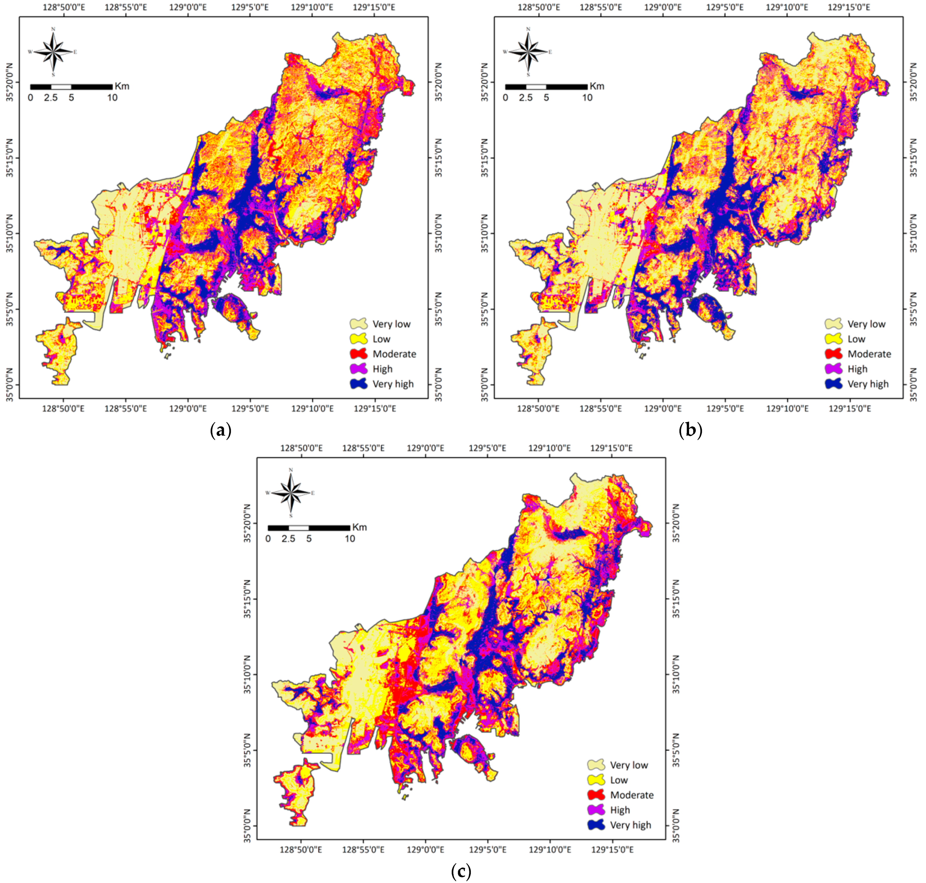
4.2. Groundwater Potential Mapping
4.2.1. Random Forest
4.2.2. Gradient Boosting Machine
4.2.3. Extreme Gradient Boosting
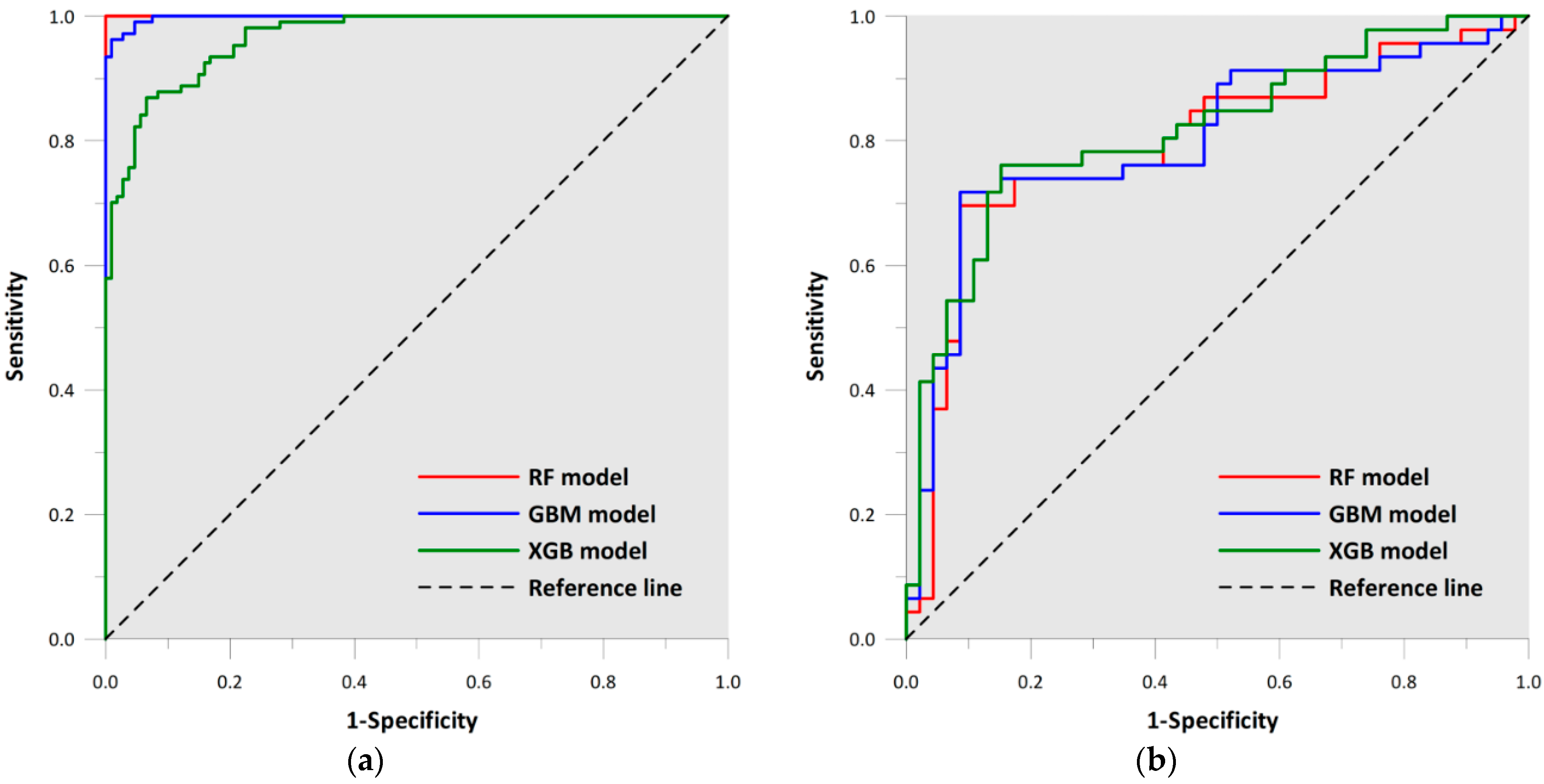
4.3. Model Validation and Comparison
5. Discussion
6. Conclusions
Author Contributions
Funding
Institutional Review Board Statement
Informed Consent Statement
Acknowledgments
Conflicts of Interest
References
- Panahi, M.; Sadhasivam, N.; Pourghasemi, H.R.; Rezaie, F.; Lee, S. Spatial prediction of groundwater potential mapping based on convolutional neural network (CNN) and support vector regression (SVR). J. Hydrol. 2020, 588, 125033. [Google Scholar] [CrossRef]
- Chen, W.; Li, H.; Hou, E.; Wang, S.; Wang, G.; Panahi, M.; Li, T.; Peng, T.; Guo, C.; Niu, C.; et al. GIS-based groundwater potential analysis using novel ensemble weights-of-evidence with logistic regression and functional tree models. Sci. Total Environ. 2018, 634, 853–867. [Google Scholar] [CrossRef] [PubMed]
- Ozdemir, A. GIS-based groundwater spring potential mapping in the Sultan Mountains (Konya, Turkey) using frequency ratio, weights of evidence and logistic regression methods and their comparison. J. Hydrol. 2011, 411, 290–308. [Google Scholar] [CrossRef]
- Pourtaghi, Z.S.; Pourghasemi, H.R. GIS-based groundwater spring potential assessment and mapping in the Birjand Township, southern Khorasan Province, Iran. Hydrogeol. J. 2014, 22, 643–662. [Google Scholar] [CrossRef]
- Mohammady, M.; Pourghasemi, H.R.; Pradhan, B. Landslide susceptibility mapping at Golestan Province, Iran: A comparison between frequency ratio, Dempster-Shafer, and weights-of-evidence models. J. Asian Earth Sci. 2012, 61, 221–236. [Google Scholar] [CrossRef]
- Pradhan, B.; Lee, S. Delineation of landslide hazard areas on Penang Island, Malaysia, by using frequency ratio, logistic regression, and artificial neural network models. Environ. Earth Sci. 2010, 60, 1037–1054. [Google Scholar] [CrossRef]
- Al-Abadi, A.M. Modeling of groundwater productivity in northeastern Wasit Governorate, Iraq using frequency ratio and Shannon’s entropy Models. Appl. Water Sci. 2017, 7, 699–716. [Google Scholar] [CrossRef]
- Liu, J.; Duan, Z. Quantitative assessment of landslide susceptibility comparing statistical index, index of entropy, and weights of evidence in the Shangnan area, China. Entropy 2018, 20, 868. [Google Scholar] [CrossRef]
- Nampak, H.; Pradhan, B.; Abd Manap, M. Application of GIS based data driven evidential belief function model to predict groundwater potential zonation. J. Hydro. 2014, 513, 283–300. [Google Scholar] [CrossRef]
- Rahmati, O.; Tahmasebipour, N.; Haghizadeh, A.; Haghizadeh, H.; Pourghasemi, H.R.; Feizizadeh, B. Evaluation of different machine learning models for predicting and mapping the susceptibility of gully erosion. Geomorphology 2017, 298, 118–137. [Google Scholar] [CrossRef]
- Chen, W.; Tsangaratos, P.; Ilia, I.; Duan, Z.; Chen, X. Groundwater spring potential mapping using population-based evolutionary algorithms and data mining methods. Sci. Total Environ. 2019, 684, 31–49. [Google Scholar] [CrossRef] [PubMed]
- Kalantar, B.; Al-Najjar, H.A.; Pradhan, B.; Saeidi, V.; Halin, A.A.; Ueda, N.; Naghibi, S.A. Optimized conditioning factors using machine learning techniques for groundwater potential mapping. Water 2019, 11, 1909. [Google Scholar] [CrossRef]
- Naghibi, S.A.; Pourghasemi, H.R.; Abbaspour, K. A comparison between ten advanced and soft computing models for groundwater qanat potential assessment in Iran using R and GIS. Theor. Appl. Climatol. 2018, 131, 967–984. [Google Scholar] [CrossRef]
- Rahmati, O.; Moghaddam, D.D.; Moosavi, V.; Kalantari, Z.; Samadi, M.; Lee, S.; Tien Bui, D. An automated python language-based tool for creating absence samples in groundwater potential mapping. Remote Sens. 2019, 11, 1375. [Google Scholar] [CrossRef]
- Al-Fugara, A.; Pourghasemi, H.R.; Al-Shabeeb, A.R.; Habib, M.; Al-Adamat, R.; Al-Amoush, H.; Collins, A.L. A comparison of machine learning models for the mapping of groundwater spring potential. Environ. Earth Sci. 2020, 79, 1–19. [Google Scholar] [CrossRef]
- Golkarian, A.; Naghibi, S.A.; Kalantar, B.; Pradhan, B. Groundwater potential mapping using C5. 0, random forest, and multivariate adaptive regression spline models in GIS. Environ. Monit. Assess 2018, 190, 149. [Google Scholar] [CrossRef]
- Chen, W.; Li, Y.; Tsangaratos, P.; Shahabi, H.; Ilia, I.; Xue, W.; Bian, H. Groundwater spring potential mapping using artificial intelligence approach based on kernel logistic regression, random forest, and alternating decision tree models. Appl. Sci. Basel 2020, 10, 425. [Google Scholar] [CrossRef]
- Park, S.; Hamm, S.Y.; Kim, J. Performance evaluation of the GIS-based data-mining techniques decision tree, random forest, and rotation forest for landslide susceptibility modeling. Sustainability 2019, 11, 5659. [Google Scholar] [CrossRef]
- Zhang, W.; Zhang, R.; Wu, C.; Goh, A.T.C.; Lacasse, S.; Liu, Z.; Liu, H. State-of-the-art review of soft computing applications in underground excavations. Geosci. Front. 2020, 11, 1095–1106. [Google Scholar] [CrossRef]
- Brédy, J.; Gallichand, J.; Celicourt, P.; Gumiere, S.J. Water table depth forecasting in cranberry fields using two decision-tree-modeling approaches. Agric. Water Manag. 2020, 233, 106090. [Google Scholar] [CrossRef]
- Tziachris, P.; Aschonitis, V.; Chatzistathis, T.; Papadopoulou, M. Assessment of spatial hybrid methods for predicting soil organic matter using DEM derivatives and soil parameters. Catena 2019, 174, 206–216. [Google Scholar] [CrossRef]
- Naghibi, S.A.; Pourghasemi, H.R.; Dixon, B. GIS-based groundwater potential mapping using boosted regression tree, classification and regression tree, and random forest machine learning models in Iran. Environ. Monit. Assess 2016, 188, 44. [Google Scholar] [CrossRef] [PubMed]
- Mosavi, A.; Hosseini, F.S.; Choubin, B.; Goodarzi, M.; Dineva, A.A.; Sardooi, E.R. Ensemble Boosting and Bagging Based Machine Learning Models for Groundwater Potential Prediction. Water Resour. Manag. 2020, 35, 23–37. [Google Scholar] [CrossRef]
- Ouedraogo, I.; Defourny, P.; Vanclooster, M. Application of random forest regression and comparison of its performance to multiple linear regression in modeling groundwater nitrate concentration at the African continent scale. Hydrogeol. J. 2019, 27, 1081–1098. [Google Scholar] [CrossRef]
- Dietterich, T. Overfitting and undercomputing in machine learning. ACM Comput. Surv. (CSUR) 1995, 27, 326–327. [Google Scholar] [CrossRef]
- Zanotti, C.; Rotiroti, M.; Sterlacchini, S.; Cappellini, G.; Fumagalli, L.; Stefania, G.A.; Nanucci, M.S.; Leoni, B.; Bonomi, T. Choosing between linear and nonlinear models and avoiding overfitting for short and long term groundwater level forecasting in a linear system. J. Hydrol. 2019, 578, 124015. [Google Scholar] [CrossRef]
- Martínez-Santos, P.; Renard, P. Mapping groundwater potential through an ensemble of big data methods. Groundwater 2020, 58, 583–597. [Google Scholar] [CrossRef]
- Jabbar, H.; Khan, R.Z. Methods to avoid over-fitting and under-fitting in supervised machine learning (comparative study). Comput. Sci. Commun. Instrum. Devices 2015, 163–172. [Google Scholar] [CrossRef]
- Cai, Z.; Jiang, B.; Lu, Z.; Liu, J.; Ma, P. isAnon: Flow-Based Anonymity Network Traffic Identification Using Extreme Gradient Boosting. In Proceedings of the 2019 International Joint Conference on Neural Networks (IJCNN), Budapest, Hungary, 14–19 July 2019; IEEE: New York City, NY, USA, 2019; pp. 1–8. [Google Scholar]
- Chen, T.; Guestrin, C. XGBoost: A scalable tree boosting system. In Proceedings of the 22nd ACM SIGKDD International Conference on Knowledge Discovery and Data Mining, San Francisco, CA, USA, 13–17 August 2016; ACM: New York, NY, USA, 2016; pp. 785–794. [Google Scholar]
- Chang, Y.C.; Chang, K.H.; Wu, G.J. Application of eXtreme gradient boosting trees in the construction of credit risk assessment models for financial institutions. Appl. Soft. Comput. 2018, 73, 914–920. [Google Scholar] [CrossRef]
- Sahin, E.K. Assessing the predictive capability of ensemble tree methods for landslide susceptibility mapping using EGBoost, gradient boosting machine, and random forest. SN Appl. Sci. 2020, 2, 1–17. [Google Scholar] [CrossRef]
- Jamali, A. Landslide hazard risk modeling in north-west of Iran using optimized machine learning models. Model Earth Syst. Environ. 2021, 7(1), 191–208. [Google Scholar] [CrossRef]
- Chen, Z.Y.; Zhang, T.H.; Zhang, R.; Zhu, Z.M.; Yang, J.; Chen, P.Y.; Ou, C.Q.; Guo, Y. Extreme gradient boosting model to estimate PM2. 5 concentrations with missing-filled satellite data in China. Atmos. Environ. 2019, 202, 180–189. [Google Scholar] [CrossRef]
- Gui, K.; Che, H.; Zeng, Z.; Wang, Y.; Zhai, S.; Wang, Z.; Luo, M.; Zhang, L.; Liao, T.; Zhao, H.; et al. Construction of a virtual PM2.5 observation network in China based on high-density surface meteorological observations using the Extreme Gradient Boosting model. Environ. Int. 2020, 141, 105801. [Google Scholar] [CrossRef] [PubMed]
- Hamedianfar, A.; Gibril, M.B.A.; Hosseinpoor, M.; Pellikka, P.K. Synergistic use of particle swarm optimization, artificial neural network, and extreme gradient boosting algorithms for urban LULC mapping from WorldView-3 images. Geocarto Int. 2020. [Google Scholar] [CrossRef]
- Georganos, S.; Grippa, T.; Vanhuysse, S.; Lennert, M.; Shimoni, M.; Wolff, E. Very high resolution object-based land use-land cover urban classification using extreme gradient boosting. IEEE Geosci. Remote S. 2018, 15, 607–611. [Google Scholar] [CrossRef]
- Zhang, W.; Wu, C.; Zhong, H.; Li, Y.; Wang, L. Prediction of undrained shear strength using extreme gradient boosting and random forest based on Bayesian optimization. Geosci. Front. 2021, 12, 469–477. [Google Scholar] [CrossRef]
- Chen, Z.; Li, H.; Goh, A.T.C.; Wu, C.; Zhang, W. Soil liquefaction assessment using soft computing approaches based on capacity energy concept. Geosciences 2020, 10, 1–19. [Google Scholar] [CrossRef]
- KMA Data Open Portal. Available online: https://kma.go.kr (accessed on 10 December 2020).
- Oh, H.J. Landslide susceptibility analysis and validation using Weight-of-Evidence model. J. Geol. Soc. Korea 2010, 46, 157–170. [Google Scholar]
- Moore, I.D.; Grayson, R.B.; Ladson, A.R. Digital terrain modelling: A review of hydrological, geomorphological, and biological applications. Hydrol. Process 1991, 5, 3–30. [Google Scholar] [CrossRef]
- Pradhan, B. Groundwater potential zonation for basaltic watersheds using satellite remote sensing data and GIS techniques. Open Geosci. 2009, 1, 120–129. [Google Scholar] [CrossRef]
- Acharjee, A.; Finkers, R.; Visser, R.G.; Maliepaard, C.J.M. Comparison of regularized regression methods for ~omics data. Metabolomics 2013, 3, 9. [Google Scholar] [CrossRef]
- Adab, H.; Morbidelli, R.; Saltalippi, C.; Moradian, M.; Ghalhari, G.A.F. Machine learning to estimate surface soil moisture from remote sensing data. Water 2020, 12, 3223. [Google Scholar] [CrossRef]
- Park, H.; Konishi, S. Robust logistic regression modelling via the elastic net-type regularization and tuning parameter selection. J. Stat. Comput. Simul. 2015, 86, 1–12. [Google Scholar] [CrossRef]
- Liu, W.; Li, Q. An efficient elastic net with regression coefficients method for variable selection of spectrum data. PLoS ONE 2017, 12, e0171122. [Google Scholar] [CrossRef]
- Giglio, C.; Brown, S.D. Using elastic net regression to perform spectrally relevant variable selection. J. Chemom. 2018, 32, e3034. [Google Scholar] [CrossRef]
- Moghaddam, D.D.; Pourghasemi, H.R.; Rahmati, O. Assessment of the contribution of geo-environmental factors to flood inundation in a semi-arid region of SW Iran: Comparison of different advanced modeling approaches. In Natural Hazards GIS Based Spatial Modeling Using Data Mining Techniques; Springer: Cham, Switzerland, 2019; pp. 59–78. [Google Scholar]
- Breiman, L. Random forests. Mach. Learn. 2001, 45, 5–32. [Google Scholar] [CrossRef]
- Micheletti, N.; Foresti, L.; Robert, S.; Leuenberger, M.; Pedrazzini, A.; Jaboyedoff, M.; Kanevski, M. Machine learning feature selection methods for landslide susceptibility mapping. Math. Geosci. 2014, 46, 33–57. [Google Scholar] [CrossRef]
- Xiao, T.; Zhu, J.; Liu, T. Bagging and boosting statistical machine translation systems. Artif. Intell. 2013, 195, 496–527. [Google Scholar] [CrossRef]
- Fan, J.; Zheng, J.; Wu, L.; Zhang, F. Estimation of daily maize transpiration using support vector machines, extreme gradient boosting, artificial and deep neural networks models. Agric. Water Manag 2020, 245, 106547. [Google Scholar] [CrossRef]
- Jenks, G.F. The Data Model Concept in Statistical Mapping. Int. Yearb. Cartogr. 1967, 7, 186–190. [Google Scholar]
- Süzen, M.L.; Doyuran, V. A comparison of the GIS based landslide susceptibility assessment methods: Multivariate versus bivariate. Environ. Geol. 2004, 45, 665–679. [Google Scholar] [CrossRef]
- Arabameri, A.; Rezaei, K.; Cerda, A.; Lombardo, L.; Rodrigo-Comino, J. GIS-based groundwater potential mapping in Shahroud plain, Iran. A comparison among statistical (bivariate and multivariate), data mining and MCDM approaches. Sci. Total Environ. 2019, 658, 160–177. [Google Scholar] [CrossRef] [PubMed]
- Osman, A.I.A.; Ahmed, A.N.; Chow, M.F.; Huang, Y.F.; El-Shafie, A. Extreme gradient boosting (Xgboost) model to predict the groundwater levels in Selangor Malaysia. Ain. Shams. Eng. J. 2021. [Google Scholar] [CrossRef]
- Rahman, A.S.; Hosono, T.; Quilty, J.M.; Das, J.; Basak, A. Multiscale groundwater level forecasting: Coupling new machine learning approaches with wavelet transforms. Adv. Water Resour. 2020, 141, 103595. [Google Scholar] [CrossRef]
- Sahour, H.; Gholami, V.; Vazifedan, M. A comparative analysis of statistical and machine learning techniques for mapping the spatial distribution of groundwater salinity in a coastal aquifer. J. Hydrol. 2020, 591, 125321. [Google Scholar] [CrossRef]
- Bedi, S.; Samal, A.; Ray, C.; Snow, D. Comparative evaluation of machine learning models for groundwater quality assessment. Environ. Monit. Assess 2020, 192, 1–23. [Google Scholar] [CrossRef] [PubMed]
- Naghibi, S.A.; Hashemi, H.; Berndtsson, R.; Lee, S. Application of extreme gradient boosting and parallel random forest algorithms for assessing groundwater spring potential using DEM-derived factors. J. Hydrol. 2020, 589, 125197. [Google Scholar] [CrossRef]
- Fan, J.; Yue, W.; Wu, L.; Zhang, F.; Cai, H.; Wang, X.; Lu, X.; Xiang, Y. Evaluation of SVM, ELM and four tree-based ensemble models for predicting daily reference evapotranspiration using limited meteorological data in different climates of China. Agric. Forest Meteorol. 2018, 263, 225–241. [Google Scholar] [CrossRef]
- Public Data Portal. Available online: https://www.data.go.kr (accessed on 28 January 2020).


| Category | Factor | Source | Scale (Resolution) | GIS and Data Type |
|---|---|---|---|---|
| Well location | - | National research paper Local research paper Field survey | - | Point |
| Topographical factors | Elevation | Topographic digital map 1 | 1:5000 | Polyline, point |
| Slope degree Slope aspect Curvature | Digital elevation model | 10 × 10 m | Raster | |
| Hydrological factors | Topographic wetness index Stream power index Distance from drainage Drainage density | Digital elevation model | 10 × 10 m | Raster |
| Geological factors | Lithology | Geology map 2 | 1:50,000 | Polygon |
| Distance from lineament Lineament density | Hill-shaded map | 10 × 10 m | Raster | |
| Distance from fault Fault density | Geology map | 1:50,000 | Polyline | |
| Land cover | Land cover | Land cover map 3 | 1:25,000 | Polygon |
| Regression Coefficient | |
|---|---|
| (Intercept) | 0.81012 |
| Elevation | −0.00009 |
| Slope degree | −0.00631 |
| Slope aspect (North) | – |
| Slope aspect (Northeast) | 0.01545 |
| Slope aspect (East) | – |
| Slope aspect (Southeast) | −0.01922 |
| Slope aspect (South) | −0.06565 |
| Slope aspect (Southwest) | – |
| Slope aspect (West) | – |
| Slope aspect (Northwest) | – |
| Curvature (Flat) | – |
| Curvature (Convex) | – |
| Topographic wetness index | −0.00095 |
| Stream power index | – |
| Distance from drainage | – |
| Drainage density | −0.03666 |
| Lithology (Alluvial rock A) | 0.06866 |
| Lithology (Alluvial rock B) | – |
| Lithology (Metamorphic rock) | – |
| Distance from lineament | −0.00004 |
| Lineament density | – |
| Distance from fault | −0.00002 |
| Fault density | – |
| Land cover (Farmland) | −0.26278 |
| Land cover (Forest) | −0.22511 |
| Land cover (Grassland) | −0.03889 |
| Land cover (Wetland) | −0.36148 |
| Land cover (Bare land) | – |
| Land cover (Water) | −0.47592 |
| Class/Model | RF | GBM | XGB | |||
|---|---|---|---|---|---|---|
| Range 1 | Area (%) 2 | Range | Area (%) | Range | Area (%) | |
| Very low | 0.005–0.215 | 24.67 | 0.026–0.182 | 34.66 | 0.313–0.398 | 25.96 |
| Low | 0.215–0.371 | 26.95 | 0.182–0.359 | 21.04 | 0.398–0.456 | 26.32 |
| Moderate | 0.371–0.542 | 20.73 | 0.359–0.559 | 14.76 | 0.456–0.520 | 20.75 |
| High | 0.542–0.729 | 15.88 | 0.559–0.762 | 14.15 | 0.520–0.595 | 14.74 |
| Very high | 0.729–0.997 | 11.76 | 0.762–0.969 | 15.39 | 0.595–0.702 | 12.23 |
| AUROC | Std. Error | Asymptotic Sig. | Asymptotic 95% Confidence Interval | |||
|---|---|---|---|---|---|---|
| Lower Bound | Upper Bound | |||||
| Calibration dataset | RF | 1.000 | 0.000 | 0.000 | 1.000 | 1.000 |
| GBM | 0.998 | 0.001 | 0.000 | 0.995 | 1.000 | |
| XGB | 0.966 | 0.010 | 0.000 | 0.946 | 0.985 | |
| Validation dataset | RF | 0.794 | 0.049 | 0.000 | 0.698 | 0.891 |
| GBM | 0.802 | 0.048 | 0.000 | 0.708 | 0.896 | |
| XGB | 0.818 | 0.045 | 0.000 | 0.730 | 0.906 | |
| % of Pixels | Training Datasets | Validation Datasets | Sum | SCAI | ||||
|---|---|---|---|---|---|---|---|---|
| No. of Wells | % of Wells | No. of Wells | % of Wells | |||||
| RF | Very low | 24.67 | 0 | 0.00 | 4 | 8.70 | 8.70 | 2.84 |
| Low | 26.95 | 0 | 0.00 | 7 | 15.22 | 15.22 | 1.77 | |
| Medium | 20.73 | 0 | 0.00 | 3 | 6.52 | 6.52 | 3.18 | |
| High | 15.88 | 8 | 7.48 | 15 | 32.61 | 40.09 | 0.40 | |
| Very high | 11.76 | 99 | 92.52 | 17 | 36.96 | 129.48 | 0.09 | |
| GBM | Very low | 34.66 | 0 | 0.00 | 4 | 8.70 | 8.70 | 3.99 |
| Low | 21.04 | 0 | 0.00 | 7 | 15.22 | 15.22 | 1.38 | |
| Medium | 14.76 | 4 | 3.74 | 2 | 4.35 | 8.09 | 1.82 | |
| High | 14.15 | 20 | 18.69 | 12 | 26.09 | 44.78 | 0.32 | |
| Very high | 15.39 | 83 | 77.57 | 21 | 45.65 | 123.22 | 0.12 | |
| XGB | Very low | 25.96 | 0 | 0.00 | 3 | 6.52 | 6.52 | 3.98 |
| Low | 26.32 | 2 | 1.87 | 6 | 13.04 | 14.91 | 1.76 | |
| Medium | 20.75 | 17 | 15.89 | 4 | 8.70 | 24.58 | 0.84 | |
| High | 14.74 | 21 | 19.63 | 15 | 32.61 | 52.23 | 0.28 | |
| Very high | 12.23 | 67 | 62.62 | 18 | 39.13 | 101.75 | 0.12 | |
Publisher’s Note: MDPI stays neutral with regard to jurisdictional claims in published maps and institutional affiliations. |
© 2021 by the authors. Licensee MDPI, Basel, Switzerland. This article is an open access article distributed under the terms and conditions of the Creative Commons Attribution (CC BY) license (http://creativecommons.org/licenses/by/4.0/).
Share and Cite
Park, S.; Kim, J. The Predictive Capability of a Novel Ensemble Tree-Based Algorithm for Assessing Groundwater Potential. Sustainability 2021, 13, 2459. https://doi.org/10.3390/su13052459
Park S, Kim J. The Predictive Capability of a Novel Ensemble Tree-Based Algorithm for Assessing Groundwater Potential. Sustainability. 2021; 13(5):2459. https://doi.org/10.3390/su13052459
Chicago/Turabian StylePark, Soyoung, and Jinsoo Kim. 2021. "The Predictive Capability of a Novel Ensemble Tree-Based Algorithm for Assessing Groundwater Potential" Sustainability 13, no. 5: 2459. https://doi.org/10.3390/su13052459
APA StylePark, S., & Kim, J. (2021). The Predictive Capability of a Novel Ensemble Tree-Based Algorithm for Assessing Groundwater Potential. Sustainability, 13(5), 2459. https://doi.org/10.3390/su13052459