Abstract
This paper proposes a practical approach to assess wind energy resource and calculate annual energy production for use on university courses in engineering. To this end, two practical exercises were designed in the open-source software GNU Octave (compatible with MATLAB) using both synthetic and field data. The script used to generate the synthetic data as well as those created to develop the practical exercises are included for the benefit of other educational bodies. With the first exercise the students learn how to characterize the wind resource at the wind turbine hub height and adjust it to the Weibull distribution. Two examples are included in this exercise: one with an appropriate fit and another where the Weibull distribution does not fit properly to the generated data. Furthermore, in this exercise, field data (gathered with a LiDAR remote sensing device) is also used to calculate shear exponents for a proper characterisation of the wind profile. The second exercise consists of the calculation of the annual energy production of a wind power plant, where the students can assess the influence of different factors (wind speed, rotor diameter, rated power, etc.) in the project. The exercises proposed can easily be implemented through either in-class or online teaching modes.
1. Introduction
With the current Strategic Energy Technology Plan (SET Plan) towards a more sustainable world [], renewable energies are playing, and will play, a key role. Wind energy is the most mature and promising of the different renewable energy sources []. A total of 650 GW of wind power is currently installed worldwide (by 2019, []), 205 GW of which is installed in Europe. Spain was the country to install the most new wind power capacity in 2019, with 2.3 GW of new onshore wind farms [].
The wind capacity installed in Spain is 26 GW []. Figure 1 depicts the annually installed wind capacity (bubble size) and the cumulative wind capacity (bubble height) in Spain, including the prospection for 2026 and 2030 (41.6 GW and 51 GW cumulative, respectively) according to the Spanish Energy and Climate National Plan (Plan Nacional Integrado de Energia y Clima, PNIEC). The difficulties experienced in the country from 2013 onward to install new wind farms, marked by regulatory changes to Feed in Tariffs (FiTs) [,], are clearly observed in Figure 1. That year, subsidies for renewable energy changed from FiTs to a capacity-based investment bonus to fix profitability at 7.5% throughout the regulated lifetime of the project [,]. Despite this, Spain holds the second position in Europe and fifth worldwide in terms of installed capacity. It can also be appreciated from Figure 1 that nearly half of the current installed capacity will have completed 15 years of operation by 2021, with around 3.5 GW being over 20 years old by then.
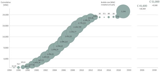
Figure 1.
Cumulative and annually installed wind capacity in Spain.
In Spain, a significant portion of the electric demand is covered by wind power generation. In this regard, Spain held the sixth position in Europe in 2019, with 21% of electricity generation covered by wind []. Denmark had the largest share (with 48%), followed by Ireland, Portugal, Germany and UK (with 33%, 27%, 26% and 22% respectively) []. Figure 2 shows the evolution from 2000 to date of the electricity demand covered by wind in Spain.
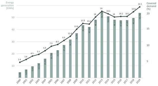
Figure 2.
Wind energy generation and electricity demand covered by wind in Spain (2000–2019).
Under this scenario, it is clear that the study of wind energy power plants must be included in engineering-related degrees. For example, in the University of Castilla–La Mancha (Spain), this topic forms part of the Electrical Engineering Degree, which is a four-year course. In this degree, renewable energies are taught in several courses during the third and fourth year, with special focus on wind and solar photovoltaic sources. A different example is found in the Technical University of Cartagena (Spain), where the topic is included in the Master’s Degree in Civil Engineering, with an academic itinerary covering wind and hydropower sources. The practical exercises proposed in the present paper are currently used with students of both these degrees.
2. Characterization of Wind Resource and Wind Power Generation
The most crucial stage of planning a wind power plant project is the wind resource assessment, as it is the basis for establishing the project’s initial feasibility and cash flow projections. Such computations are key for obtaining financing, usually from banks or banking consortia. High-resolution wind resource data are now accessible in many countries and regions, and a preliminary study can usually be completed by leveraging such data. Once the study area is determined, the first step is to obtain wind data collected close to the site. Wind resource data sets are collected on a met tower over the course of a year. When met towers are lower than the wind turbine hub height, the data collected must be scaled up to the expected height. Different equations are used that take into account the terrain on which the wind farm is to be located.
The next step is to model the wind resource in the area, which is achieved by characterising the wind resource data sets at the turbine’s hub height. Frequency distributions, such as the Weibull and Rayleigh density functions, are typically employed to this end [,,]. The annual energy production (AEP) is then calculated using the fitted density function at the turbine hub height and the wind turbine power curve. A number of other elements are also taken into account when estimating energy production, including the average air density for the site, where the power curve is adjusted for the site density, assumed to be constant throughout the year. If there are significant changes in the seasonal variation of air density, a method to correct the AEP is advisable, as proposed in []. Despite the availability of software packages, such as WindFarmer®, WindPRO®, WAsP®, Meteodyn®, WindSim®, which can be used to assess wind resource and energy production and to develop wind farms, students should be trained in the basic elements of wind resource assessment and AEP calculation.
Given that the available energy and the AEP vary with the cube of the wind speed and are directly related to the financial viability of wind power plant projects, characterizing the wind resource is a key process []. Wind turbine power production, P, can be estimated using the widely used expression:
where is the air density ( standard conditions for dry air at sea level, defined as 15 °C and mbar), is the power coefficient, A is the rotor swept area, and v is the wind speed at hub height [].
Wind is typically a commodity that, from a temporal and geographical perspective, varies greatly. As the wind resource at a particular location may differ from one year to the next, the wind speed data collected for assessment might correspond to an atypical year, thus affecting the viability calculations for the particular wind farm project. Wind power generation, aggregated at country level, can also present inter-annual oscillations [,].
Figure 3 shows the impact of monthly wind power generation in Spain between 2014 and 2020, which clearly shows a seasonal pattern. The inter-annual variability of wind can be seen in the difference between, for example, September 2014 and 2018, and October 2018, which yielded the lowest monthly production (slightly less than 15%), and March 2018 and November 2019, which were the months with the highest wind power generation (over 40% of the total rated installed capacity). Before that, 2013 was an excellent year for wind resource across the peninsula, and Spain was the first country in the world in which wind power was the leading technology in terms of electricity production. This scenario has not as yet been repeated, although the notable drop in new wind projects since 2013 is also partly to blame for this (Figure 1).
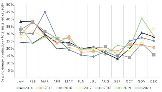
Figure 3.
Wind energy generation covering the electricity demand in Spain from 2014 to 2020.
Furthermore, obstacles and surface roughness on the ground create shear stresses which lead to a significant braking effect on wind, whereas high above the ground in the undisturbed air layers of geostrophic wind (approximately 5 km above ground) the surface conditions have no impact. This phenomenon is known as the atmospheric boundary layer, and also as vertical wind shear, due to the effects on the wind speed vertical profile []. On flat terrain and with a neutrally stratified atmosphere, where thermal boundary effects can be neglected, the logarithmic wind profile is a good estimation for the vertical wind shear []:
where the reference wind speed is measured at height , v is the wind speed at height H, and z is the roughness length, which can be obtained depending on the characteristics of the terrain (Table 1).

Table 1.
Roughness length, z [].
An exponential approximation can also be applied to model the wind profile, where the exponent varies with the type of terrain (Equation (3)), also known as the power law. When the value of is equal to , it is commonly referred to as the one-seventh power law. In the United States, the power law (Equation (3)) is typically employed, while in Europe the logarithmic law (Equation (2)) is more commonly used [].
where v is the wind speed at height H, is the wind speed at height , and is the friction coefficient (also known as Hellman exponent or shear exponent). This coefficient is a function of the topography at a specific site, with a value of being frequently assumed for open land. This value can be obtained according to the terrain characteristics (Table 2).
Table 2.
Shear exponent, [].
Then, in order to estimate the AEP, the wind speed data series at the wind turbine hub height is used. In this regard, the use of mathematical functions to model the wind speed distribution over a period of time, typically a year, is recommended in the literature. The Weibull distribution is the function traditionally used for modeling wind speed distributions in wind energy studies [,,]. For a specific location and a certain wind speed (v), the Weibull probability density function is given by []:
where is the Weibull scale parameter (with units equal to the wind speed units) and is the dimensionless Weibull shape parameter.
As previously mentioned, different reference wind speed frequency distributions can be used, such as the Weibull and Rayleigh density functions, with the latter being a particular Weibull distribution with a shape factor () of 2. Given the considerable degree of random variation in 10-min or hourly mean wind speed measurements over a year, multiple studies have proposed Weibull distributions for wind resource modeling [,,,]. Consequently, Weibull distributions have commonly been applied to wind speed characterization but primarily when wind speed data are restricted to a specific location with a single meteorological tower (also known as a met mast). Nonetheless, and despite only one Weibull distribution being able to provide adequate representations, wind speed distributions are not efficiently characterized by one Weibull distribution in all locations. The effects of diverse wind climates, such as the variability of wind distribution according to wind direction or a strong underlying seasonal component stemming from changes in insolation throughout the year as a result of the tilt of the Earth’s axis of rotation during summer or winter, can necessitate a more complex representation based on a double-peaked bi-Weibull distribution [,,], with different scale and shape factors according to the seasons []. In addition, other probability density functions have recently been posited in the specific literature for such purposes [,].
As recommended in the International Electrotechnical Commission (IEC) Standard to measure the power performance of electricity-producing wind turbines [], the Weibull density function profile can be used to calculate the AEP of wind turbines and wind farms. Thus, data represented in a typical discrete wind speed histogram can be presented as a continuous function, called a probability density function. The defining elements of the histogram include the area under the curve being equal to a unit, and the ease of the process to find the probability of the wind being between two specific speeds, where it is only necessary to compute the area under the curve between the two wind speeds. Following the aforementioned standard, the annual energy production (AEP) is estimated assuming that wind turbines have an availability of 100%.
The AEP is calculated using Equation (5):
where, is the number of hours in one year (8760), N is the number of bins, is the wind speed in the upper limit in bin i, is the power output for such wind speed, and is the Weibull cumulative probability distribution function for wind speed.
In addition, the capacity factor (CF) and the equivalent full load hours (EFLH) are two common parameters used for the techno-economic assessment of wind power plants []. The CF is the ratio between the energy produced by the wind power plant over one year and the energy it would have produced if operating continuously at its rated power () during that year, Equation (6). The corresponding EFLH is obtained by multiplying the CF coefficient by the total number of hours in a year, Equation (7), i.e., it is the number of hours the wind power plant ought to operate at its rated power to generate the same amount of energy as it did in one year.
3. Description of the Synthetic and Field Data
Both synthetic and field wind data are used in this work to develop the proposed exercises. For the benefit of other educational bodies, the script used to generate the synthetic data is described as follows and included in the Appendix A as Listing A1, where step-by-step instructions can be found. Although it is more convenient to use field measurements for this purpose, the difficulty in accessing such sorts of data makes it useful to generate artificial data series.
The script created to generate random wind data provides a two-column file containing one year of ten-minute wind speed values (second column) sorted per wind direction (first column) at a chosen height. This script can be implemented using different Weibull factors depending on the wind direction. In this way, common small variations can be reproduced (i.e., appropriate Weibull fit), but also significant variations, like those occurring in complex orography (upstream) for different wind directions (i.e., non-appropriate single Weibull fit). For the latter kind of data, students learn and practice that fitting a single Weibull distribution regardless of the wind direction would lead to poor adjustments and hence inaccurate AEP estimations, whereas using a distribution for each wind direction bin leads to a better agreement. It should be mentioned that, while the generated data distribution might seem real, its temporal evolution is totally random and unrealistic and should never be used as a time series.
In addition, a three-month field data set has also been used in one of the exercises and can be provided to other educational bodies under request. For this data set, a measurement campaign was performed in a Spanish wind power plant for a continuous period of three months during winter. Specifically, the wind power plant is located in the region of Higueruela, which is one of the areas with the best wind resource in Spain []. Ten-minute wind speed and wind direction measurements were collected with a LiDAR device (Figure 4). The measurements were taken at ten different heights using the LiDAR device, these being: 40 m, 50 m, 62 m, 72 m, 85 m, 95 m, 110 m, 140 m, 160 m, and 200 m.
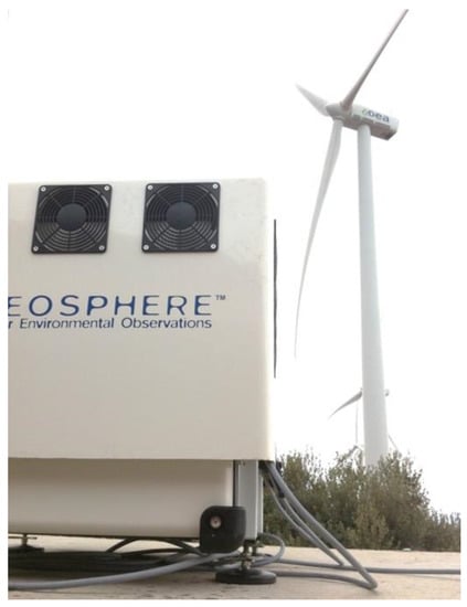
Figure 4.
LiDAR installed in a wind farm.
4. Practical Exercises in GNU Octave
Two practical exercises are proposed for the students to assess the wind resource and to calculate the AEP, respectively, as previously described. These exercises are implemented in GNU Octave [] (open-source software compatible with MATLAB), presented as follows. The G80 Siemens-Gamesa wind turbine will be used for the calculations.
4.1. Practical Exercise 1: Wind Speed Characterization
The aim of this exercise is for students to develop the skills to characterize the wind resource at different sites using the Weibull distribution, while noticing the importance of land roughness. The variation of wind speed with height is studied by proposing the characterization of the wind resource at the wind turbine hub height using both the logarithmic and the exponential laws (Equations (2) and (3), respectively) for different terrains.
For this exercise, the students are provided with two different sets of synthetic data and one set of field data. The first set of synthetic data shows an appropriate Weibull distribution fit (MastMetData1), while the second set does not (MastMetData2). A third set of field data is used to calculate instantaneous values of . Thus, the objectives of this exercise are:
- To adjust the Weibull distribution to different synthetic data sets (proper fit and non-proper fit) and obtain the scale () and shape () parameters.
- To obtain the wind speed values at the G80 wind turbine hub height (set to 90 m for academic purposes) for three different terrains: flat, medium and complex, using both the logarithmic and power laws.
- To obtain instantaneous values of using the field data set.
To accomplish Objective 1, the students are asked to:
- Obtain scale and factor Weibull parameters for the data set.
- Jointly plot the data using a histogram and the Weibull curve obtained.
- Assess graphically whether the Weibull curve fits the histogram data.
The script developed for Objective 1 is included in the Appendix A as Listing A2, and the results are shown in Figure 5 and Figure 6. The MastMetData1 set is represented in Figure 5a, showing an appropriate Weibull fit. This case allows students to learn the procedure of fitting by calculating the scale and factor Weibull parameters. The second case, shown in Figure 5b, shows an example in which the Weibull distribution does not properly fit to the data, and thus, should not be used to represent the data.
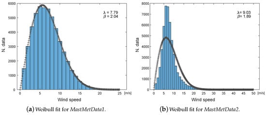
Figure 5.
Weibull distribution and histogram for different synthetic data sets at 20 m height. N. data refers to the number of samples.
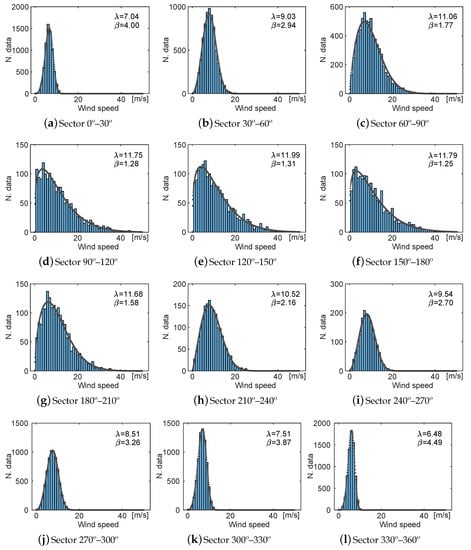
Figure 6.
Weibull fit and histogram per wind sector for MastMetData2. N. data refers to the number of samples.
For some sites, wind may be represented by a sum of different Weibull distributions as wind characteristics change depending on the wind’s direction or the season. In order for the students to comprehend this phenomenon and the associated calculation problem, the students are asked to classify the MastMetData2 set by wind direction and to re-calculate the scale and factor Weibull parameters for each sub-set. To accomplish this task, the wind data will be sorted into twelve sectors, following the procedure commonly implemented by commercial tools (e.g., Global Wind Atlas® [] or WAsP® []). The results are shown in Figure 6. In this figure, students can assess which wind directions are predominant, like those found in Figure 6a,l, or which are less common, like those seen in Figure 6d–g.
Next, Objective 2 is accomplished using Equations (2) and (3), as shown in the script given in Listing A3 of the Appendix A. The results are shown in Figure 7 and Figure 8. The wind speed obtained at the hub height for different terrains is depicted in Figure 7a using the logarithmic law (Equation (2), for the specified roughness lengths) and Figure 7b using the power law (Equation (3), for the specified friction coefficients). In both graphs, the variation of wind speed from 20 m to 90 m height for different types of terrain (flat, medium and complex) is shown for one day. The full data set at the wind turbine hub height for the different terrains and their adjusted Weibull distributions are shown in Figure 8a,b using the logarithmic law and the power law, respectively.
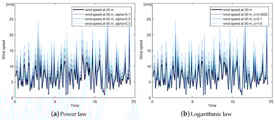
Figure 7.
Wind speed of MastMetData1 at the reference height (20 m) and hub height (90 m) for different terrains.
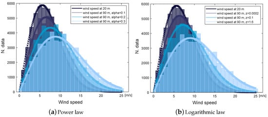
Figure 8.
Wind speed histograms and Weibull functions of MastMetData1 at the reference height (20 m) and hub height (90 m) for different terrains. N. data refers to the number of samples.
Finally, to accomplish Objective 3, field data collected with the LiDAR device for a period of three months is used. The script is included as Listing A4 in the Appendix A. The friction coefficient () may vary significantly according to atmosphere stability, year, month, hour of the day, or even wind direction and wind speed values. Figure 9 shows actual wind speed variations at different heights from the field data set. As can be seen, for high wind speeds (Figure 9a) the wind speed increases with height. This is not the case for lower wind speeds (Figure 9b). Thus, this objective is intended to help students understand the complexity of this phenomenon by analysing the variation of the friction coefficients for different pairs of heights.
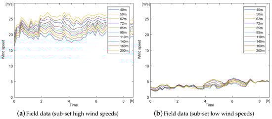
Figure 9.
Actual wind speeds at different heights (data collected with the LiDAR device July 2010).
To this end, instantaneous values are calculated using Equation (3) and the field data set. The results are shown in Figure 10. As can be seen, lower shear exponents are measured during daytime while larger shear exponents are found during nighttime. Actually, during daytime the temperature near the ground is greater than at upper heights due to solar irradiation, which causes an unstable atmosphere in which the wind profile is flat (i.e., the difference between wind speeds is small at different heights and hence low shear exponents are observed). In contrast, during nighttime, due to thermal stratification, the atmosphere becomes stable and hence no-flat wind profiles are measured (high shear exponents). Thus, with this exercise, the students can assess the complexity of obtaining wind speeds at the wind turbine hub height taking into account the characteristics of the terrain, and therefore the importance of carrying out measurement campaigns at the hub height or the rotor swept area range.
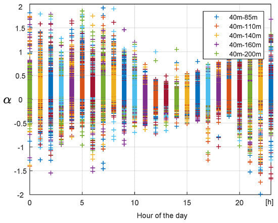
Figure 10.
Instantaneous values for different pairs of heights obtained using field data.
4.2. Practical Exercise 2: Calculation of the AEP
The aim of this exercise is for students to develop the skills to estimate the expected AEP of a wind power plant so they can assess the project economically. They should also develop the skills to analyse the results critically and to assess the influence of different factors in the AEP (wind speed, rotor diameter, nominal power, etc.). To this end, the AEP, CF and EFLH will be calculated using both the wind measurements and the Weibull fit. The scripts developed for this exercise are included in the Appendix A as Listing A5 for MastMetData1 and Listing A6 for MastMetData2.
Thus, the objectives of this exercise are:
- To plot in the same figure the distribution of wind (both measured and fitted) and the G80 wind turbine power curve to discuss the importance of relative changes in the wind distribution and in the characteristics of the power curve (cut-in and cut-out speeds, rotor area, maximum power, …).
- To estimate the AEP using the fitted Weibull function and the measured data. To discuss the differences between both estimations.
- To calculate the CF and EFLH.
Objective 1 is designed for students to assess graphically the influence of the wind distribution and the wind turbine power curve when calculating the AEP, functions multiplied as per Equation (5). To this end, both functions are plotted jointly in Figure 11 for each data set. In this figure, students can observe that the probability of having wind speeds above 15 m/s is low for the sites analysed. Thus, a small increase in the nominal power of the wind turbine (e.g., from 2 MW to 2.5 MW or 3 MW) would not lead to a substantial rise in the AEP. However, there is a notable occurrence of wind speeds located in the parabolic part of the power curve, meaning that increasing the power in this part of the curve (through greater blades for instance) would lead the AEP to increase significantly.
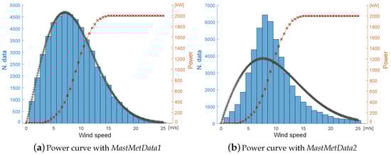
Figure 11.
G80 wind turbine power curve compared to the different wind data sets. N. data refers to the number of samples.
The results obtained for Objectives 2 and 3 are presented in Table 3 and Table 4 for MatMestData1 and MatMestData2, respectively. As can be seen in Table 3, very similar results are achieved when using the Weibull distribution and the measured data for MatMestData1. This is because this data set meets an appropriate Weibull adjustment. However, that is not the case for the second data set (see Table 4), where the Weibull distribution does not show an appropriate fit. Thus, significant differences are obtained in the AEP, CF and EFLH when using the measured data and the non-appropriate Weibull fit. In this case, as previously explained, it is necessary to classify the wind measurements per wind direction (see Figure 6) and use those twelve Weibull functions to calculate the AEP, CF and EFLH.
Table 3.
Annual Energy Production, CF and EFLH calculated for MatMestData1.
Table 4.
Annual Energy Production, CF and EFLH calculated for MatMestData2.
5. Conclusions
Renewable energies have emerged as a key element in moving towards a more sustainable world. Of these energies, wind is the most mature and promising. Thus, it is highly important for engineers to acquire the relevant competences in the field of wind energy. To this end, the present work shows two exercises for students to acquire practical knowledge in developing wind energy power plants. The first exercise focuses on the wind resource and Weibull adjustment that can be used, as per the IEC Standard, to estimate the AEP of a wind power plant, included in the second exercise. As an extension of the proposed exercises, other distributions could be implemented to assess the wind resource, such as the bimodal Weibull, Kappa or Wakeby distributions []. Besides, the statistical test , could be implemented to validate the adjustment quantitatively. Furthermore, the calculations proposed in these exercises can also be utilised for research purposes. Both exercises have been developed using the open-source software GNU Octave (compatible with MATLAB), and all the scripts are included in the Appendix for the benefit of other educational bodies.
These exercises are used in the Electric Engineering Degree at the University of Castilla–La Mancha, and the MSc Degree in Civil Engineering at the Technical University of Cartagena. For several years, lecturers have observed fruitful outcomes from the students and have received their positive feedback. Although these universities conduct their teaching activities face-to-face at their engineering schools, these exercises can easily be implemented on online-mode courses too. This was indeed the case during the COVID-19 pandemic, when the different goals of the exercises were satisfactorily achieved by the students, as in previous years.
Author Contributions
E.A. prepared the submission and developed some sections and the results of the paper. A.H.-E. developed other sections and supported the development of the results. A.V.-R. and S.M.-M. developed the scripts and supported the paper development. E.G.-L. supervised all the work. All authors have read and agreed to the published version of the manuscript.
Funding
This research work was partially supported by the Council of Communities of Castilla–La Mancha (SBPLY/19/180501/000287) and the European Union FEDER.
Data Availability Statement
The three-month field data set used in Exercise 1– Objective 3 can be provided to other educational bodies under request. All the scripts are included in the Appendix A and can also be provided as source files if requested.
Conflicts of Interest
The authors declare no conflict of interest.
Nomenclature
| P | Power production |
| Power coefficient | |
| Air density | |
| A | Rotor swept area |
| v | Wind speed |
| H | Height |
| z | Roughness length |
| Shear Exponent | |
| Weibull shape parameter | |
| Weibull scale parameter | |
| Hours in a year | |
| Annual Energy Production | |
| Capacity Factor | |
| Equivalent Full Load Hours | |
| Rated power of wind power plant |
Appendix A. Scripts in GNU Octave
Listing A1.
Script to generate synthetic wind speed data.
Listing A1.
Script to generate synthetic wind speed data.


Listing A2.
Script to develop objective 1 of Practical Exercise 1.
Listing A2.
Script to develop objective 1 of Practical Exercise 1.


Listing A3.
Script to develop objective 2 of Practical Exercise 1.
Listing A3.
Script to develop objective 2 of Practical Exercise 1.


Listing A4.
Script to develop objective 3 of Practical Exercise 1.
Listing A4.
Script to develop objective 3 of Practical Exercise 1.


Listing A5.
Script to develop objectives 1 to 3 of Practical Exercise 2 for appropriate Weibull distribution.
Listing A5.
Script to develop objectives 1 to 3 of Practical Exercise 2 for appropriate Weibull distribution.


Listing A6.
Script to develop objectives 1 to 3 of Practical Exercise 2 for non–appropriate Weibull distribution.
Listing A6.
Script to develop objectives 1 to 3 of Practical Exercise 2 for non–appropriate Weibull distribution.


Listing A7.
Script for “wblfit2” function to be used in OCTAVE.
Listing A7.
Script for “wblfit2” function to be used in OCTAVE.


References
- United Nations. Kyoto Protocol to the United Nations Framework Convention on Climate Change; Framework Convention on Climate Change: Kyoto, Japan, 1998. [Google Scholar]
- Honrubia-Escribano, A.; Gomez-Lazaro, E.; Fortmann, J.; Sorensen, P.; Martin-Martinez, S. Generic dynamic wind turbine models for power system stability analysis: A comprehensive review. Renew. Sustain. Energy Rev. 2018, 81, 1939–1952. [Google Scholar] [CrossRef]
- Joyce Lee, F.Z. Global Wind Report 2019; Technical Report; Global Wind Energy Council: Brussels, Belgium, 2020. [Google Scholar]
- Komusanac, I.; Brindley, G.; Fraile, D. Wind Energy in Europe in 2019; Technical Report; Wind Europe: Brussels, Belgium, 2020. [Google Scholar]
- Asociación Empresarial Eólica. Technical Report Eólica 19; Technical Report; AEE: Madrid, Spain, 2020. [Google Scholar]
- Artigao, E.; Martin-Martinez, S.; Ceña, A.; Honrubia-Escribano, A.; Gomez-Lazaro, E. Failure rate and downtime survey of wind turbines located in Spain. IET Renew. Power Gener. 2020. [Google Scholar] [CrossRef]
- Ramirez, F.J.; Honrubia-Escribano, A.; Gomez-Lazaro, E.; Pham, D.T. The role of wind energy production in addressing the European renewable energy targets: The case of Spain. J. Clean. Prod. 2018, 196, 1198–1212. [Google Scholar] [CrossRef]
- Rosales-Asensio, E.; Borge-Diez, D.; Blanes-Peiró, J.J.; Pérez-Hoyos, A.; Comenar-Santos, A. Review of wind energy technology and associated market and economic conditions in Spain. Renew. Sustain. Energy Rev. 2019, 101, 415–427. [Google Scholar] [CrossRef]
- Edmunds, C.; Martín-Martínez, S.; Browell, J.; Gómez-Lázaro, E.; Galloway, S. On the participation of wind energy in response and reserve markets in Great Britain and Spain. Renew. Sustain. Energy Rev. 2019, 115, 109360. [Google Scholar] [CrossRef]
- El Sistema Eléctrico Español 2019; Technical Report; Red Eléctrica de España: Alcobendas, Spain, 2019.
- Zhang, M. Wind Resource Assessment and Micro-Siting: Science and Engineering; John Wiley & Sons Singapore Pte. Ltd.: Singapore, 2015. [Google Scholar]
- Manwell, J.F.; McGowan, J.G.; Rogers, A.L. Wind Energy Explained: Theory, Design and Application; Wiley: Chichester, UK, 2009. [Google Scholar]
- Wang, L.; Liu, J.; Qian, F. Frequency Distribution Model of Wind Speed Based on the Exponential Polynomial for Wind Farms. Sustainability 2019, 11, 665. [Google Scholar] [CrossRef]
- Ulazia, A.; Ibarra-Berastegi, G.; Sáenz, J.; Carreno-Madinabeitia, S.; González-Rojí, S.J. Seasonal correction of offshore wind energy potential due to air density: Case of the Iberian Peninsula. Sustainability 2019, 11, 3648. [Google Scholar] [CrossRef]
- Wan, Y. Long-Term Wind Power Variability; Technical Report; National Renewable Energy Laboratory: Golden, CO, USA, 2012.
- Alharthi, Y.Z.; Siddiki, M.K.; Chaudhry, G.M. Resource assessment and techno-economic analysis of a grid-connected solar PV-wind hybrid system for different locations in Saudi Arabia. Sustainability 2018, 10, 3690. [Google Scholar] [CrossRef]
- Burton, T.; Jenkins, N.; Sharpe, D.; Bossanyi, E. Wind Energy Handbook; John Wiley & Sons: Hoboken, NJ, USA, 2011. [Google Scholar]
- Masters, G. Renewable and Efficient Electric Power Systems; John Wiley & Sons: Hoboken, NJ, USA, 2004. [Google Scholar]
- Lavidas, G.; K Kaldellis, J. Assessing Renewable Resources at the Saronikos Gulf for the Development of Multi-Generation Renewable Systems. Sustainability 2020, 12, 9169. [Google Scholar] [CrossRef]
- Hennessey, J.P., Jr. Some aspects of wind power statistics. J. Appl. Meteorol. 1977, 16, 119–128. [Google Scholar] [CrossRef]
- Conradsen, K.; Nielsen, L.; Prahm, L. Review of Weibull statistics for estimation of wind speed distributions. J. Clim. Appl. Meteorol. 1984, 23, 1173–1183. [Google Scholar] [CrossRef]
- Lun, I.Y.; Lam, J.C. A study of Weibull parameters using long-term wind observations. Renew. Energy 2000, 20, 145–153. [Google Scholar] [CrossRef]
- Justus, C.; Hargraves, W.; Mikhail, A.; Graber, D. Methods for estimating wind speed frequency distributions. J. Appl. Meteorol. 1978, 17, 350–353. [Google Scholar] [CrossRef]
- Gualtieri, G.; Secci, S. Extrapolating wind speed time series vs. Weibull distribution to assess wind resource to the turbine hub height: A case study on coastal location in Southern Italy. Renew. Energy 2014, 62, 164–176. [Google Scholar] [CrossRef]
- Carta, J.; Ramirez, P. Analysis of two-component mixture Weibull statistics for estimation of wind speed distributions. Renew. Energy 2007, 32, 518–531. [Google Scholar] [CrossRef]
- Akpinar, S.; Akpinar, E.K. Estimation of wind energy potential using finite mixture distribution models. Energy Convers. Manag. 2009, 50, 877–884. [Google Scholar] [CrossRef]
- Akdağ, S.; Bagiorgas, H.; Mihalakakou, G. Use of two-component Weibull mixtures in the analysis of wind speed in the Eastern Mediterranean. Appl. Energy 2010, 87, 2566–2573. [Google Scholar] [CrossRef]
- Chang, T.P. Performance comparison of six numerical methods in estimating Weibull parameters for wind energy application. Appl. Energy 2011, 88, 272–282. [Google Scholar] [CrossRef]
- Chang, T.P. Estimation of wind energy potential using different probability density functions. Appl. Energy 2011, 88, 1848–1856. [Google Scholar] [CrossRef]
- IEC 61400-12-1:2017. Wind Energy Generation Systems—Part 12-1: Power Performance Measurements of Electricity Producing Wind Turbines; International Electrotechnical Commission: Geneva, Switzerland, 2017. [Google Scholar]
- Villena-Ruiz, R.; Ramirez, F.J.; Honrubia-Escribano, A.; Gomez-Lazaro, E. A techno-economic analysis of a real wind farm repowering experience: The Malpica case. Energy Convers. Manag. 2018, 172, 182–199. [Google Scholar] [CrossRef]
- Eaton, J.W.; Bateman, D.; Hauberg, S.; Wehbring, R. GNU Octave Version 4.4.0 Manual: A High-Level Interactive Language for Numerical Computations; Eaton, J.W., Ed.; The Free Software Foundation: Boston, MA, USA, 2018. [Google Scholar]
- Davis, N.; Badger, J.; Hahmann, A.N.; Hansen, B.O.; Olsen, B.T.; Mortensen, N.G.; Heathfield, D.; Onninen, M.; Lizcano, G.; Lacave, O. Global Wind Atlas v3. DTU Wind Energy: Roskilde, Denmark, 2019. [Google Scholar] [CrossRef]
- Mortensen, N.G. Wind Resource Assessment Using the WAsP Software; DTU Wind Energy: Roskilde, Denmark, 2018. [Google Scholar]
- Morgan, E.C.; Lackner, M.; Vogel, R.M.; Baise, L.G. Probability distributions for offshore wind speeds. Energy Convers. Manag. 2011, 52, 15–26. [Google Scholar] [CrossRef]
Publisher’s Note: MDPI stays neutral with regard to jurisdictional claims in published maps and institutional affiliations. |
© 2021 by the authors. Licensee MDPI, Basel, Switzerland. This article is an open access article distributed under the terms and conditions of the Creative Commons Attribution (CC BY) license (http://creativecommons.org/licenses/by/4.0/).