
Optimization of a Novel Urban Growth Simulation Model Integrating an Artificial Fish Swarm Algorithm and Cellular Automata for a Smart City


Abstract
1. Introduction
2. Case Study Area and Data
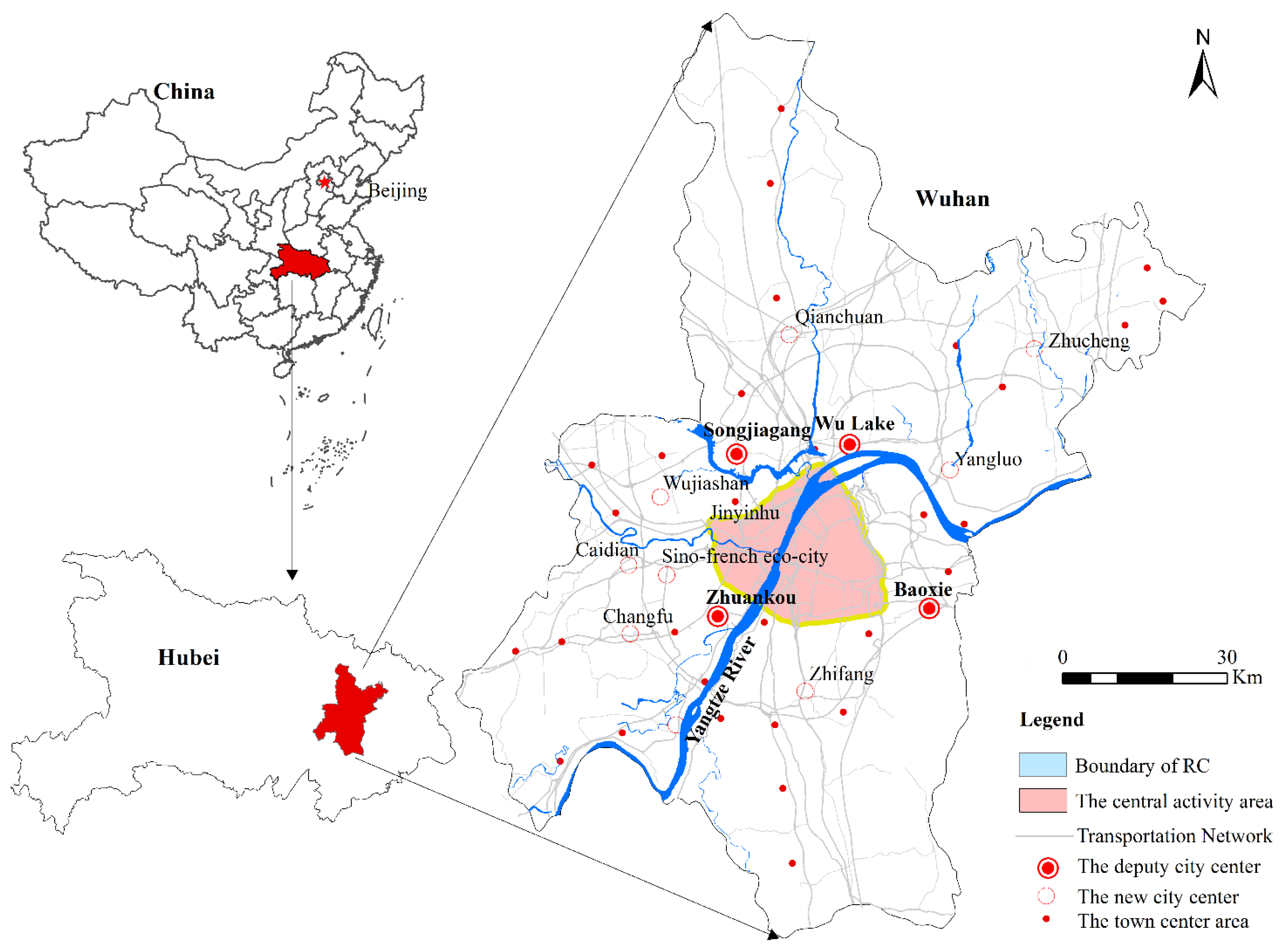
2.1. Study Area
2.2. Data Acquisitions
3. Methodology
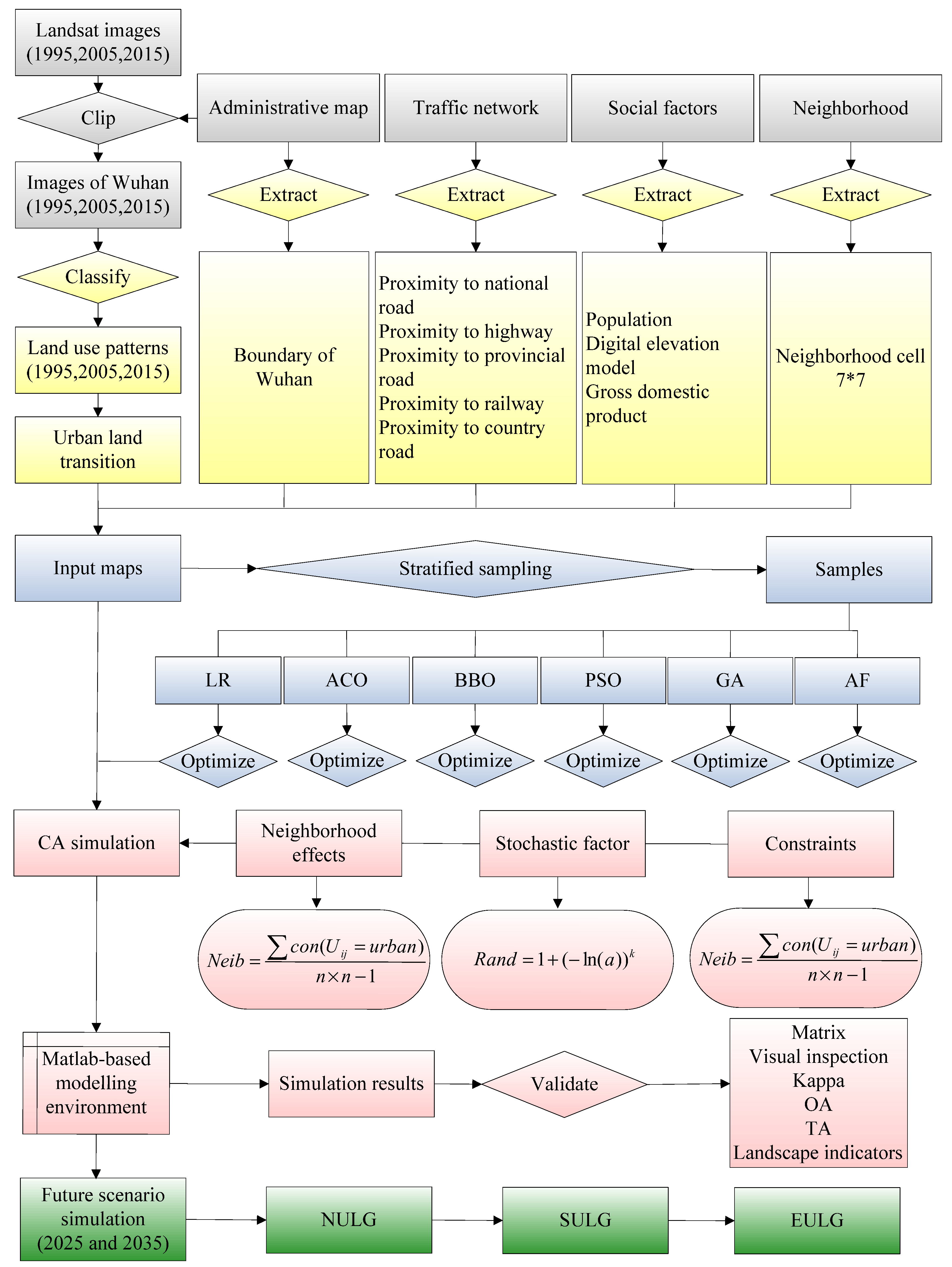
- (1)
- Preparation of training data: the land-use data are reclassified and divided into urban land, non-urban land, and water. Each variable is then associated with each grid cell in the study area, and the Euclidean distance is used to calculate the distance to each level of road.
- (2)
- Optimized the parameter of each variable: In the MATLAB R2014 a software environment, the acquired data samples are used to obtain the weight of each variable by the six methods (BLR-CA, ACO-CA-CA, BBO-CA, PSO-CA, GA-CA, and AFSA-CA).
- (3)
- Calibrating CA models for urban growth land simulation: the conversion probabilities acquired by the six methods are applied to calibrate the urban land expansion model with the cell neighborhoods, the constraint coefficients, and random factors.
- (4)
- Accuracy assessment: The performance of the calibrated models is evaluated using a visual comparison, the Kappa coefficient, and the figure of merit (FoM), and landscape indicators.
- (5)
- Future scenario simulation: the proposed model (AFSA-CA) is applied to simulate the urban land growth in 2025 and 2035 under different scenarios.
3.1. The Urban CA Model
3.2. Six Optimization Methods
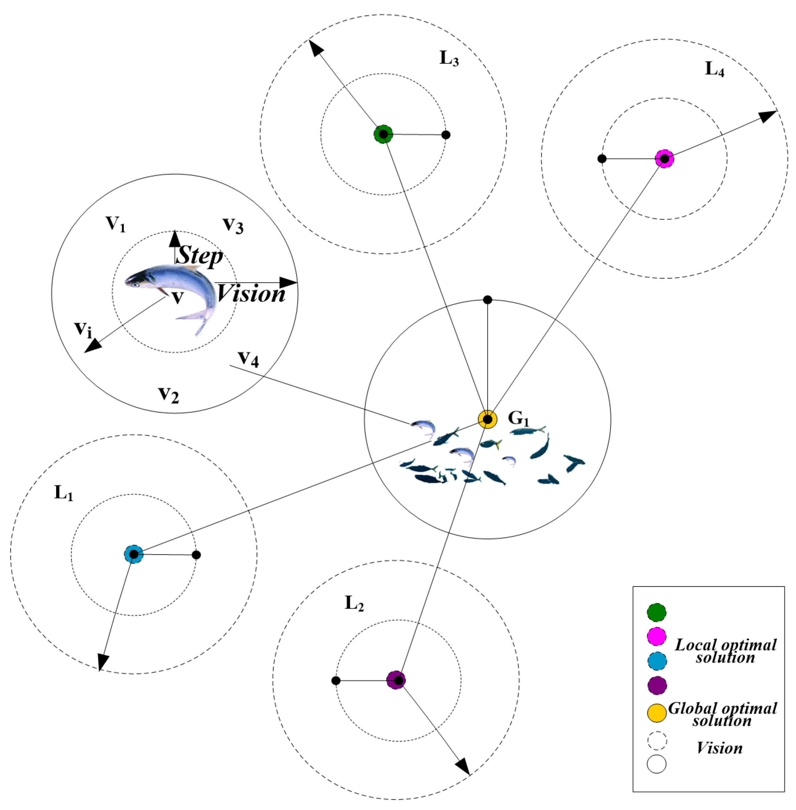
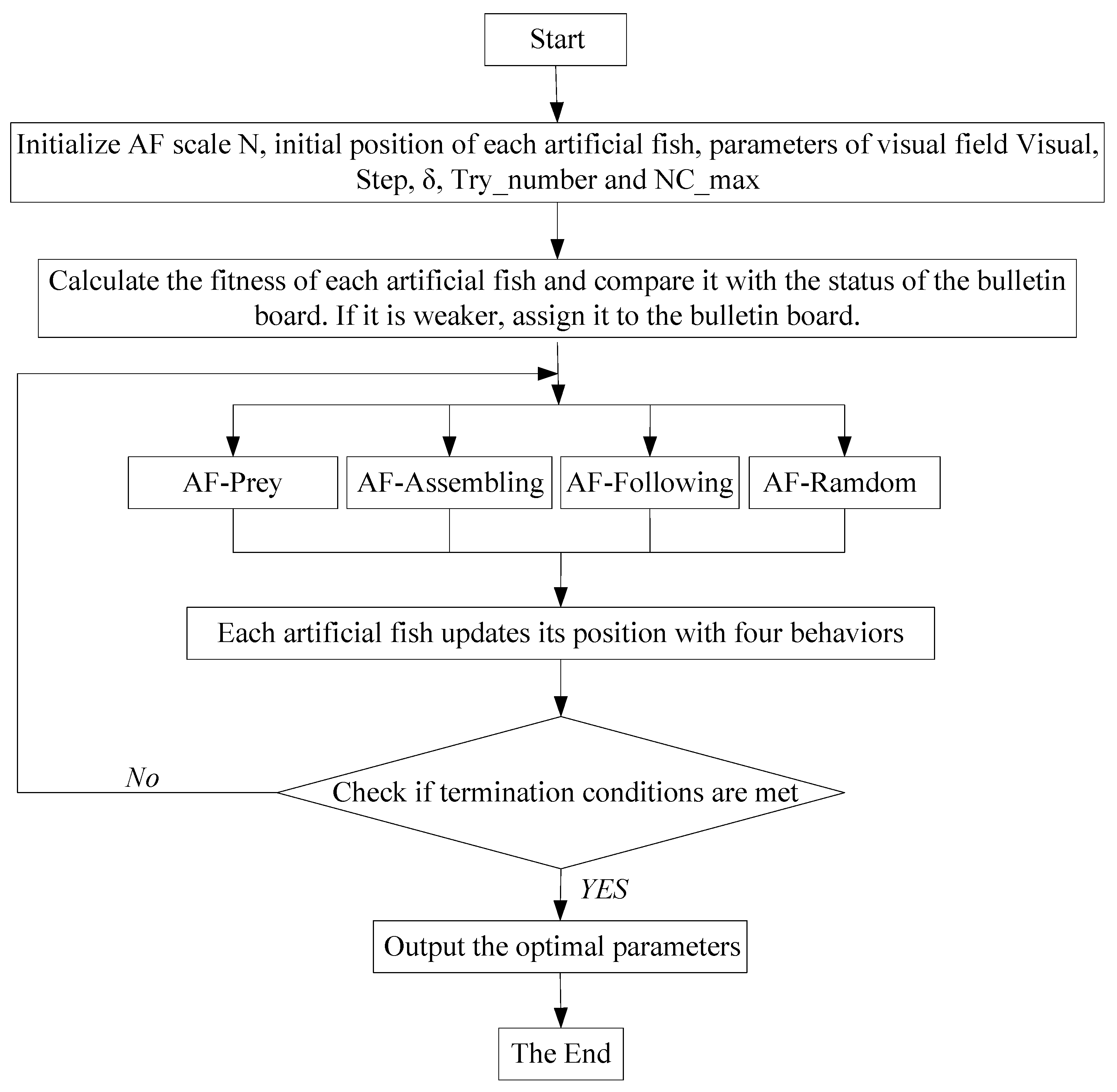
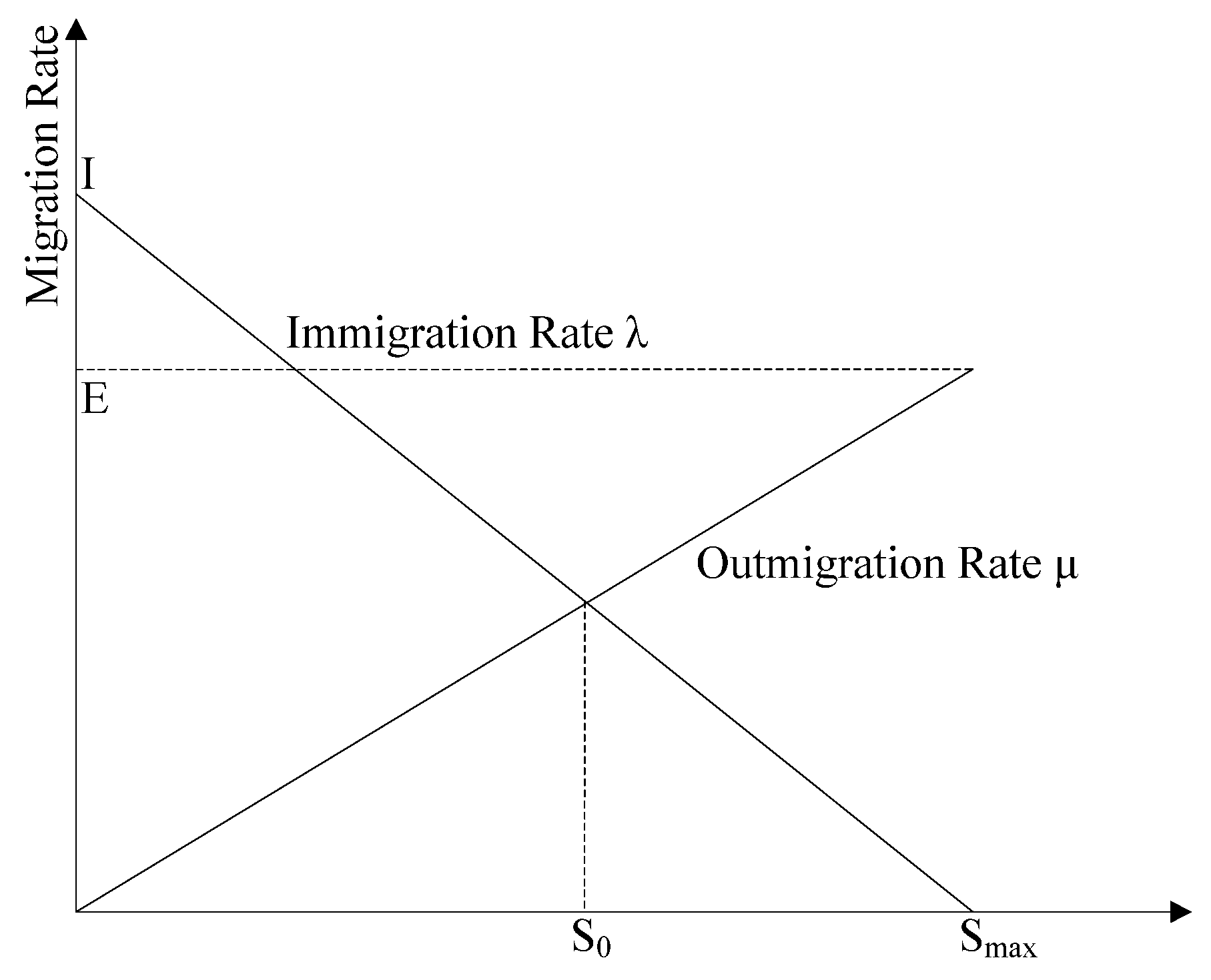
3.2.1. AFSA Optimization Process
- (1)
- AF-Prey
- (2)
- AF-Assembling
- (3)
- AF-Following
- (4)
- AF-Random
3.2.2. Five Optimization Methods for Comparison
- (1)
- Animals tend to form small social groups. Thus, individuals need to rely on the power of group cooperation to survive and perform activities.
- (2)
- In terms of information exchange, social groups survive through information exchange. The ACO algorithm interacts with the information of pheromones, while the PSO and AFSA algorithms directly interact with the current position information.
- (3)
- Positive feedback is required, and effective suppression is also required. For example, the ACO algorithm relies on the pheromone evaporation mechanism and AFSA introduces a “crowding” factor.
- (4)
- The algorithms avoid falling into local extrema and introduce random factors. For example, the ACO algorithm selects paths randomly, a random number is used in PSO, and random steps are used in AFSA.
3.3. Accuracy Assessment
4. Results
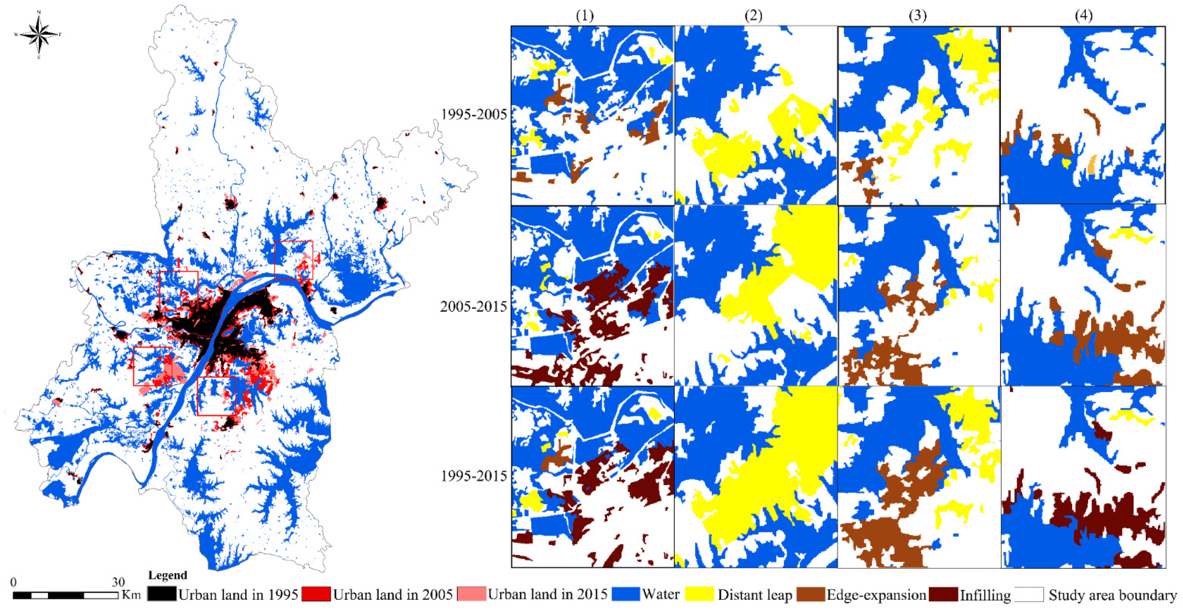
4.1. Actual Urban Growth Characteristics during the Periods of 1995–2005 and 2005–2015
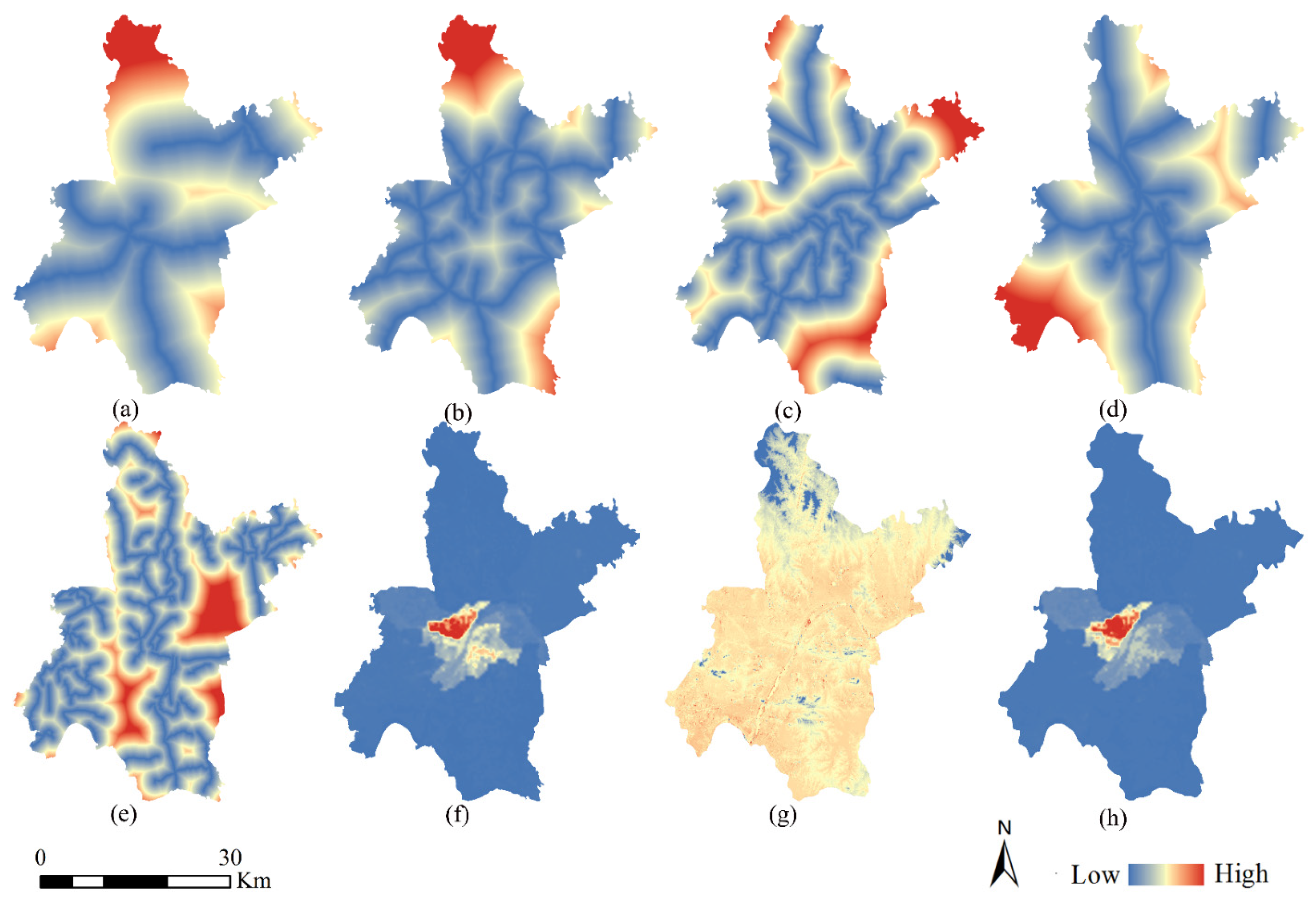
4.2. Optimized Parameters of Driving Factors in Six Methods
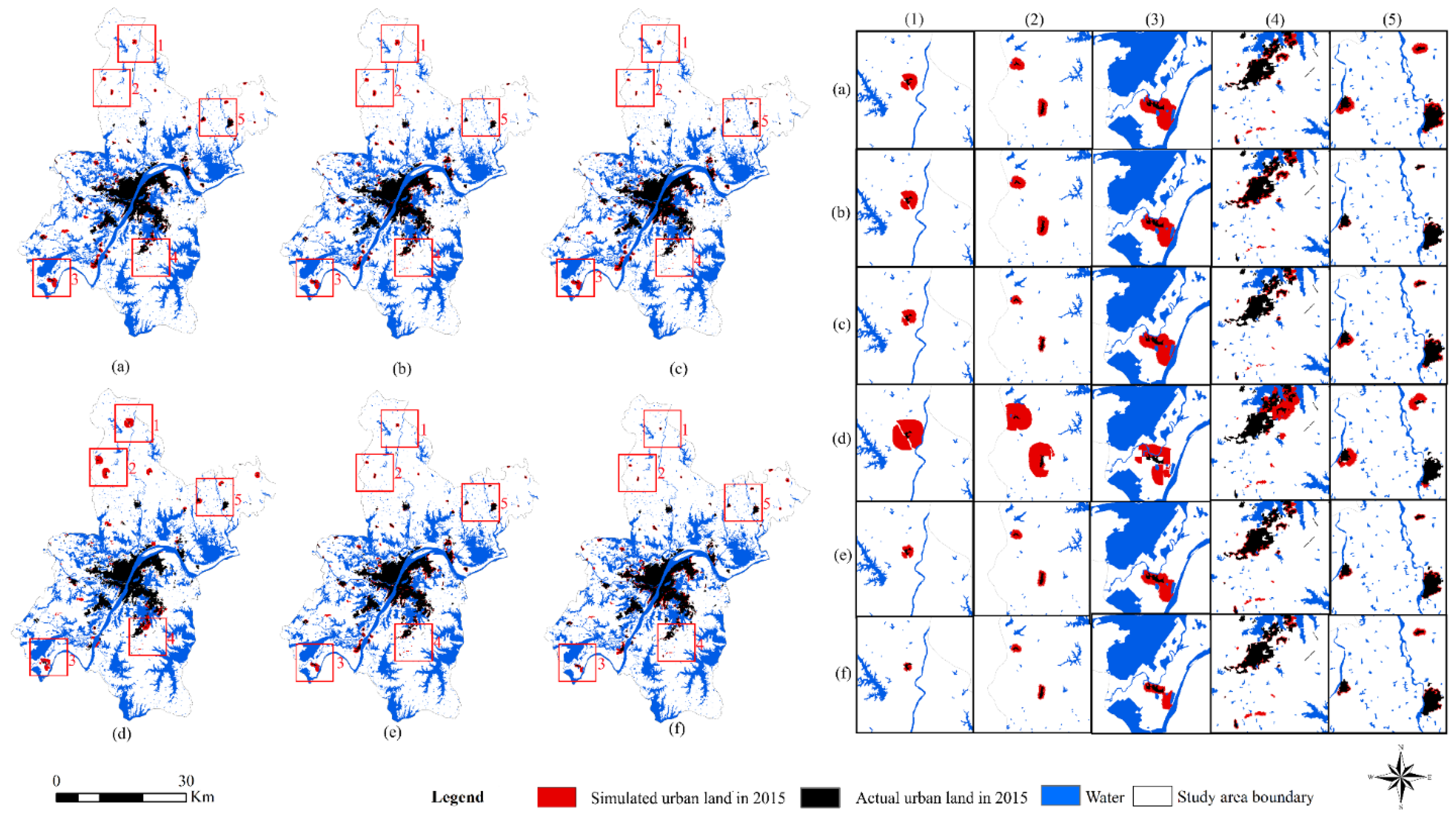
4.3. Simulated Results of Six Optimized CA Models
5. Discussion and Implications
5.1. Effects of Differences Models on Urban Growth Simulation
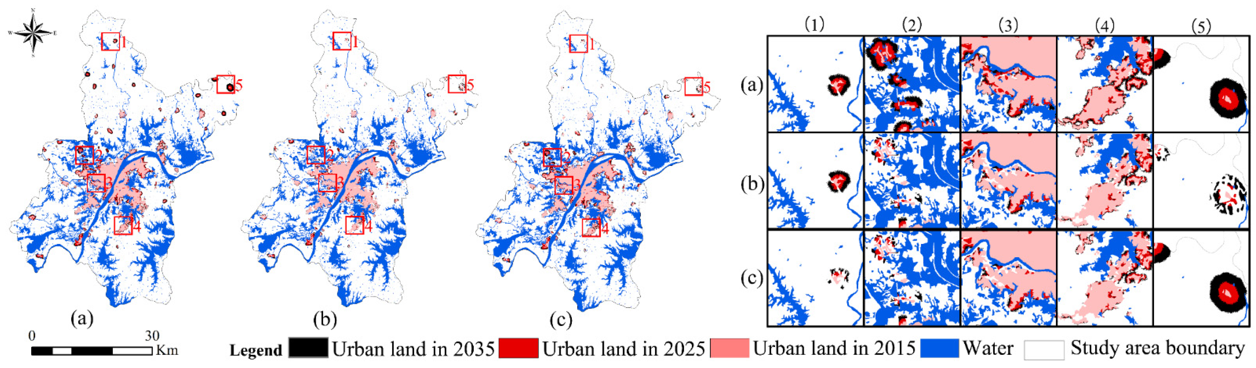
5.2. Future Scenario Simulation for Wuhan in 2025 and 2035
5.3. Role of Urban Growth Simulation for Smart City
6. Conclusions
Author Contributions
Funding
Data Availability Statement
Conflicts of Interest
Abbreviations
| CA | the cellular automaton |
| BLR | binary logistic regression |
| GAs | genetic algorithms |
| ACOs | ant colony algorithms |
| PSO | particle swarm optimization |
| BBO | biogeography-based optimization |
| AFSA | artificial fish swarm algorithm |
| Neib | neighborhoods |
| Suit | constraints |
| Rand | random factors |
| UA | urban accuracy |
| TA | total accuracy |
| NP | the number of urban patches |
| PARA_MN | average perimeter ratio |
| ENN_MN | average Euclidean nearest neighbor distance |
| POP | population |
| DEM | digital elevation model |
| GDP | gross domestic product |
| LUD1 | Land-use in 1995 |
| LUD2 | Land-use in 2005 |
| LUD3 | Land-use in 2015 |
| D-nat | Distance to national road |
| D-hig | Distance to highway |
| D-pro | Distance to provincial road |
| D-rai | Distance to railway |
| D-cou | Distance to country road |
| NEI | Neighhood cell |
| NULG | natural urban land growth without any restrictions |
| SULG | sustainable urban land growth with cropland protection and ecological security |
| EULG | economic urban land growth with sustainable development and economic development in the core area |
References
- United Nations. World Urbanization Prospects: The 2018 Revision; United Nations Department of Economic and Social Affairs: New York, NY, USA, 2019.
- Zhang, W.; Li, W.; Zhang, C.; Hanink, D.M.; Liu, Y.; Zhai, R. Analyzing horizontal and vertical urban expansions in three East Asian megacities with the SS-coMCRF model. Landsc. Urban Plan. 2018, 177, 114–127. [Google Scholar] [CrossRef]
- Chuang, U.; Cho, J.; Yun, J. Urbanization effect on the observed change in mean monthly temperatures between 1951–1980 and 1971–2000 in Korea. Clim. Chang. 2011, 66, 127–136. [Google Scholar] [CrossRef]
- Lee, D.; Choe, H. Estimating the Impacts of Urban Expansion on Landscape Ecology: Forestland Perspective in the Greater Seoul Metropolitan Area. J. Urban Plan. Dev. 2011, 137, 425–437. [Google Scholar] [CrossRef]
- Zhou, Y.; Huang, B.; Wang, J.; Chen, B.; Kong, H.; Norford, L. Climate-Conscious Urban Growth Mitigates Urban Warming: Evidence from Shenzhen, China. Environ. Sci. Technol. 2019. [Google Scholar] [CrossRef]
- Camero, A.; Alba, E. Smart City and information technology: A review. Cities 2019, 93, 84–94. [Google Scholar] [CrossRef]
- Clarke, K.C.; Hoppen, S. A self-modifying cellular automaton model of historical urbanization in the San Francisco Bay area. Environ. Plan. 1997, 24, 247–261. [Google Scholar] [CrossRef]
- Xu, T.; Gao, J.; Coco, G.; Wang, S. Urban expansion in Auckland, New Zealand: A GIS simulation via an intelligent self-adapting multiscale agent-based model. Int. J. Geogr. Inf. Sci. 2020, 34, 1–24. [Google Scholar] [CrossRef]
- Chen, G.; Li, X.; Liu, X.; Chen, Y.; Liang, X.; Leng, J.; Xu, X.; Liao, W.; Qiu, Y.a.; Wu, Q.; et al. Global projections of future urban land expansion under shared socioeconomic pathways. Nat. Commun. 2020, 11, 1–12. [Google Scholar] [CrossRef]
- Yang, Y.; Bao, W.; Liu, Y. Scenario simulation of land system change in the Beijing-Tianjin-Hebei region. Land Use Policy 2020, 96, 104677. [Google Scholar] [CrossRef]
- He, J.; Li, X.; Yao, Y.; Hong, Y.; Jinbao, Z. Mining transition rules of cellular automata for simulating urban expansion by using the deep learning techniques. Int. J. Geogr. Inf. Sci. 2018, 32, 2076–2097. [Google Scholar] [CrossRef]
- Wu, F.; Webster, C.J. Simulation of Land Development through the Integration of Cellular Automata and Multicriteria Evaluation. Environ. Plann. B Plan. Des. 1998, 25, 103–126. [Google Scholar] [CrossRef]
- Naghibi, F.; Delavar, M.R.; Pijanowski, B. Urban Growth Modeling Using Cellular Automata with Multi-Temporal Remote Sensing Images Calibrated by the Artificial Bee Colony Optimization Algorithm. Sensors 2016, 16, 2122. [Google Scholar] [CrossRef]
- Naghibi, F.; Delavar, M. Discovery of Transition Rules for Cellular Automata Using Artificial Bee Colony and Particle Swarm Optimization Algorithms in Urban Growth Modeling. ISPRS Int. J. Geo-Inf. 2016, 5, 241. [Google Scholar] [CrossRef]
- Wang, H.; Xia, C.; Zhang, A.; Zhang, W. Calibrating urban expansion cellular automata using biogeography based optimization. Geomat. Inf. Sci. Wuhan Univ. 2017, 42, 1323–1329. [Google Scholar]
- Al-Kofahi, S.D.; Hammouri, N.; Sawalhah, M.N.; Al-Hammouri, A.A.; Aukour, F.J. Assessment of the urban sprawl on agriculture lands of two major municipalities in Jordan using supervised classification techniques. Arab. J. Geosci. 2018, 11, 45. [Google Scholar] [CrossRef]
- Rienow, A.; Goetzke, R. Supporting SLEUTH—Enhancing a cellular automaton with support vector machines for urban growth modeling. Comput. Environ. Urban Syst. 2015, 49, 66–81. [Google Scholar] [CrossRef]
- Wu, H.; Li, Z.; Clarke, K.C.; Shi, W.; Fang, L.; Lin, A.; Zhou, J. Examining the sensitivity of spatial scale in cellular automata Markov chain simulation of land use change. Int. J. Geogr. Inf. Sci. 2019, 33, 1040–1061. [Google Scholar] [CrossRef]
- Hagenauer, J.; Omrani, H.; Helbich, M. Assessing the performance of 38 machine learning models: The case of land consumption rates in Bavaria, Germany. Int. J. Geogr. Inf. Sci. 2019, 33, 1399–1419. [Google Scholar] [CrossRef]
- Farswan, P.; Bansal, J.C. Fireworks-inspired biogeography-based optimization. Soft Comput. 2018, 23, 7091–7115. [Google Scholar] [CrossRef]
- Li, X.; Lin, J.; Chen, Y.; Liu, X.; Ai, B. Calibrating cellular automata based on landscape metrics by using genetic algorithms. Int. J. Geogr. Inf. Sci. 2013, 27, 594–613. [Google Scholar] [CrossRef]
- Yazdani, D.; Nasiri, B.; Sepas-Moghaddam, A.; Meybodi, M.; Akbarzadeh-Totonchi, M. mNAFSA: A novel approach for optimization in dynamic environments with global changes. Swarm Evol. Comput. 2014, 18, 38–53. [Google Scholar] [CrossRef]
- Li, X.L. An Optimi zing Method Based on Autonomous Animats: Fish-swarm Algorithm. Syst. Eng. Theory Pract. 2002, 22, 32–38. [Google Scholar]
- Li, X.-L.; Xue, Y.-C.; Lu, F.; Tian, G.-H. Parameter estimation method based-on artificial fish school algorithm. J. Shandong Univ. 2004, 34, 84–87. [Google Scholar]
- Neshat, M.; Sepidnam, G.; Sargolzaei, M.; Toosi, A.N. Artificial fish swarm algorithm: A survey of the state-of-the-art, hybridization, combinatorial and indicative applications. Artif. Intell. Rev. 2012, 42, 965–997. [Google Scholar] [CrossRef]
- Gao, Y.; Guan, L.; Wang, T.; Sun, Y. A novel artificial fish swarm algorithm for recalibration of fiber optic gyroscope error parameters. Sensors 2015, 15, 10547–10568. [Google Scholar] [CrossRef]
- Chen, W.; Feng, Y.-Z.; Jia, G.-F.; Zhao, H.-T. Application of Artificial Fish Swarm Algorithm for Synchronous Selection of Wavelengths and Spectral Pretreatment Methods in Spectrometric Analysis of Beef Adulteration. Food Anal. Methods 2018, 11, 2229–2236. [Google Scholar] [CrossRef]
- Shao, H.; Jiang, H.; Zhao, H.; Wang, F. A novel deep autoencoder feature learning method for rotating machinery fault diagnosis. Mech. Syst. Signal Process. 2017, 95, 187–204. [Google Scholar] [CrossRef]
- Zhao, W.; Du, C.; Jiang, S. An adaptive multiscale approach for identifying multiple flaws based on XFEM and a discrete artificial fish swarm algorithm. Comput. Methods Appl. Mech. Eng. 2018, 339, 341–357. [Google Scholar] [CrossRef]
- Azad, M.A.K.; Rocha, A.M.A.C.; Fernandes, E.M.G.P. Improved binary artificial fish swarm algorithm for the 0–1 multidimensional knapsack problems. Swarm Evol. Comput. 2014, 14, 66–75. [Google Scholar] [CrossRef]
- Zhang, Z.; Wang, K.; Zhu, L.; Wang, Y. A Pareto improved artificial fish swarm algorithm for solving a multi-objective fuzzy disassembly line balancing problem. Expert Syst. Appl. 2017, 86, 165–176. [Google Scholar] [CrossRef]
- Liu, X.; Liu, H.; Yang, J.; Litak, G.; Cheng, G.; Han, S. Improving the bearing fault diagnosis efficiency by the adaptive stochastic resonance in a new nonlinear system. Mech. Syst. Signal Process. 2017, 96, 58–76. [Google Scholar] [CrossRef]
- He, Q.; Hu, X.; Ren, H.; Zhang, H. A novel artificial fish swarm algorithm for solving large-scale reliability-redundancy application problem. ISA Trans. 2015, 59, 105–113. [Google Scholar] [CrossRef]
- Luo, T.; Tan, R.; Kong, X.; Zhou, J. Analysis of the Driving Forces of Urban Expansion Based on a Modified Logistic Regression Model: A Case Study of Wuhan City, Central China. Sustainability 2019, 11, 2207. [Google Scholar] [CrossRef]
- Chen, W.; Zhao, H.; Li, J.; Zhu, L.; Wang, Z.; Zeng, J. Land use transitions and the associated impacts on ecosystem services in the Middle Reaches of the Yangtze River Economic Belt in China based on the geo-informatic Tupu method. Sci. Total Environ. 2019, 701, 134690. [Google Scholar] [CrossRef] [PubMed]
- Feng, Y.; Tong, X. Using exploratory regression to identify optimal driving factors for cellular automaton modeling of land use change. Environ. Monit. Assess. 2017, 189, 515. [Google Scholar] [CrossRef] [PubMed]
- Zhang, B.; Wang, H.; He, S.; Xia, C. Analyzing the effects of stochastic perturbation and fuzzy distance transformation on Wuhan urban growth simulation. Trans. GIS 2020, 24, 1779–1798. [Google Scholar] [CrossRef]
- Wu, F. Calibration of stochastic cellular automata: The application to rural-urban land conversions. Int. J. Geogr. Inf. Sci. 2002, 16, 795–818. [Google Scholar] [CrossRef]
- Wang, L.G.; Shi, Q.H.; Hong, Y. Hybrid Optimization Algorithm of PSO and AFSA. Comput. Eng. 2010, 36, 176–178. [Google Scholar] [CrossRef]
- Wu, F. An Experiment on the Generic Polycentricity of Urban Growth in a Cellular Automatic City. Environ. Plan. B Plan. Des. 1998, 25, 731–752. [Google Scholar] [CrossRef]
- Simon, D. Biogeography-Based Optimization. IEEE Trans. Evol. Comput. 2008, 12, 702–713. [Google Scholar] [CrossRef]
- Shan, J.; Alkheder, S.; Wang, J. Cellular automata urban growth model calibration with genetic algorithms. Photogramm. Eng. Remote Sens. 2007, 74, 1267–1277. [Google Scholar] [CrossRef]
- He, Q.; Tan, S.; Yin, C.; Zhou, M. Collaborative optimization of rural residential land consolidation and urban construction land expansion: A case study of Huangpi in Wuhan, China. Comput. Environ. Urban Syst. 2019, 74, 218–228. [Google Scholar] [CrossRef]
- Pontius, R.G.; Boersma, W.; Castella, J.-C.; Clarke, K.; de Nijs, T.; Dietzel, C.; Duan, Z.; Fotsing, E.; Goldstein, N.; Kok, K.; et al. Comparing the input, output, and validation maps for several models of land change. Ann. Reg. Sci. 2007, 42, 11–37. [Google Scholar] [CrossRef]
- Chen, Y.; Li, X.; Wang, S.; Liu, X.; Ai, B. Simulating Urban Form and Energy Consumption in the Pearl River Delta Under Different Development Strategies. Ann. Assoc. Am. Geogr. 2013, 103, 1567–1585. [Google Scholar] [CrossRef]
- Li, X.; Liu, X.; Yu, L. A systematic sensitivity analysis of constrained cellular automata model for urban growth simulation based on different transition rules. Int. J. Geogr. Inf. Sci. 2014, 28, 1317–1335. [Google Scholar] [CrossRef]
- Jiang, C.; Wan, L.; Sun, Y.; Li, Y. The Application of PSO-AFSA Method in Parameter Optimization for Underactuated Autonomous Underwater Vehicle Control. Math. Probl. Eng. Eng. 2017, 2017, 1–14. [Google Scholar] [CrossRef]
- Ma, C.; He, R. Green wave traffic control system optimization based on adaptive genetic-artificial fish swarm algorithm. Neural Comput. Appl. 2015, 31, 2073–2083. [Google Scholar] [CrossRef]
- Park, S.; Jeon, S.; Kim, S.; Choi, C. Prediction and comparison of urban growth by land suitability index mapping using GIS and RS in South Korea. Landsc. Urban Plan. 2011, 99, 104–114. [Google Scholar] [CrossRef]
- Mustafa, A.; Van Rompaey, A.; Cools, M.; Saadi, I.; Teller, J. Addressing the determinants of built-up expansion and densification processes at the regional scale. Urban Stud. 2018, 55, 3279–3298. [Google Scholar] [CrossRef]
- Blum, C.; Dorigo, M. The Hyper-Cube Framework for Ant Colony Optimization. IEEE Trans. Syst. Man Cybern. Part B 2004, 34, 1161–1172. [Google Scholar] [CrossRef] [PubMed]
- Li, X.; Yeh, A.G.-O. Modelling sustainable urban development by the integration of constrained cellular automata and GIS. Int. J. Geogr. Inf. Sci. 2000, 14, 131–152. [Google Scholar] [CrossRef]
- White, R. Cellular automata and fractal urban form: A cellular modelling approach to the evolution of urban land-use patterns. Environ. Plan. A Plan. Des. 1993, 25, 1175–1199. [Google Scholar] [CrossRef]
- Yao, Y.; Liu, X.; Li, X.; Liu, P.; Hong, Y.; Zhang, Y.; Mai, K. Simulating urban land-use changes at a large scale by integrating dynamic land parcel subdivision and vector-based cellular automata. Int. J. Geogr. Inf. Sci. 2017, 31, 2452–2479. [Google Scholar] [CrossRef]
- He, Q.; Liu, Y.; Zeng, C.; Chaohui, Y.; Tan, R. Simultaneously simulate vertical and horizontal expansions of a future urban landscape: A case study in Wuhan, Central China. Int. J. Geogr. Inf. Sci. 2017, 31, 1907–1928. [Google Scholar] [CrossRef]
- Ke, X.; Zheng, W.; Zhou, T.; Liu, X. A CA-based land system change model: LANDSCAPE. Int. J. Geogr. Inf. Sci. 2017, 31, 1798–1817. [Google Scholar] [CrossRef]
- Xia, C.; Zhang, A.; Wang, H.; Zhang, B. Modeling urban growth in a metropolitan area based on bidirectional flows, an improved gravitational field model, and partitioned cellular automata. Int. J. Geogr. Inf. Sci. 2019, 33, 877–899. [Google Scholar] [CrossRef]
- Yang, J.; Gakenheimer, R. Assessing the transportation consequences of land use transformation in urban China. Habitat Int. 2007, 31, 345–353. [Google Scholar] [CrossRef]
- Wang, M.; Krstikj, A.; Koura, H. Effects of urban planning on urban expansion control in Yinchuan City, Western China. Habitat Int. 2017, 64, 85–97. [Google Scholar] [CrossRef]
- Chai, B.; Seto, K.C. Conceptualizing and characterizing micro-urbanization: A new perspective applied to Africa. Landsc. Urban Plan. 2019, 190, 103595. [Google Scholar] [CrossRef]
- Yuan, M.; Huang, Y.; Shen, H.; Li, T. Effects of urban form on haze pollution in China: Spatial regression analysis based on PM2.5 remote sensing data. Appl. Geogr. 2018, 98, 215–223. [Google Scholar] [CrossRef]
- Luo, M. Motivity of Spatial Urban Expansion by Cellular Automata Model —Taking Analysis of Wuhan Spatial Urban Expansion as an Example. Geomat. Inf. Sci. Wuhan Univ. 2005, 30, 52–55. [Google Scholar] [CrossRef]
- Yu, D. Self-organization characteristics of urban extension and the planning effect evaluation A case study of Beijing. Geogr. Res. 2016, 35, 353–362. [Google Scholar] [CrossRef]
- Wang, T.; Han, Q.; de Vries, B. A semi-automatic neighborhood rule discovery approach. Appl. Geogr. 2017, 88, 73–83. [Google Scholar] [CrossRef]
- Xu, T.; Gao, J.; Li, Y. Machine learning-assisted evaluation of land use policies and plans in a rapidly urbanizing district in Chongqing, China. Land Use Policy 2019, 87, 104030. [Google Scholar] [CrossRef]


| Dataset | Type | Year | Full Meaning | Acquisition Method | Purpose |
|---|---|---|---|---|---|
| LUD1 | GRID | 1995 | Land-use in 1995 | Reclassification | To create the land-use patterns |
| LUD2 | GRID | 2000 | Land-use in 2000 | Reclassification | To create the land-use patterns |
| LUD3 | GRID | 2015 | Land-use in 2015 | Reclassification | To create the land-use patterns |
| D-nat | Shpfile | 2015 | Distance to national road | Euclidean distance | Global driving factor |
| D-hig | Shpfile | 2015 | Distance to highway | Euclidean distance | Global driving factor |
| D-pro | Shpfile | 2015 | Distance to provincial road | Euclidean distance | Global driving factor |
| D-rai | Shpfile | 2015 | Distance to railway | Euclidean distance | Global driving factor |
| D-cou | Shpfile | 2015 | Distance to country road | Euclidean distance | Global driving factor |
| POP | GRID | 2015 | Population | Resample | Global driving factor |
| DEM | GRID | 2015 | Digital elevation model | Resample | Global driving factor |
| GDP | GRID | 2015 | Gross domestic product | Resample | Global driving factor |
| NEI | GRID | - | Neighhood cell | - | Local driving factors |
| Set Parameters | Expression Form | Significance |
|---|---|---|
| Total number | N | A set of candidate solutions |
| Try_number | Try_number | Maximum number of heuristics per move |
| Iterations | NC | Number of repetitions |
| Max-iterations | NC_max | Maximum number of repetitions |
| The artificial fish movement distance | step | Distance of each step |
| Crowding factor | δ | Judgment on merits of the environment |
| Field of view | vision | Range of vision |
| Algorithm 1: The Pseudo-code of the AF Algorithm |
|---|
| Procedure the initial artificial fish swarm |
| Set gen = 1 While gen <= MAXgen Print the food consistency and positions for fishes |
| Assess the print result |
| Calculate the behavior Float AF-prey Float AF-follow Float AF-swarm Float AF-random If the maximum of the dependent > the best of the gen Produce the best solution |
| And if |
| Define the best solution Record current best solution Gen = gen + 1 |
| End repeat |
| Variable | BLR-CA | ACO | BBO-CA | PSO-CA | GA-CA | AFSA-CA |
|---|---|---|---|---|---|---|
| D-nat | −4.3100 | −10.1042 | −5.2933 | −3.9468 | −16.4928 | −4.9734 |
| D-hig | −5.4880 | −0.5539 | −8.2734 | −4.1205 | −2.1272 | −1.1546 |
| D-pro | −4.6970 | 1.9882 | 4.0829 | 1.0876 | −3.2782 | −19.5246 |
| D-rai | −10.238 | −3.1680 | −13.6067 | −1.5529 | −15.2515 | −2.1672 |
| D-cou | 0.9850 | 6.0789 | −6.9345 | 8.4651 | −18.3324 | −1.2427 |
| POP | 1.6110 | −3.1961 | 12.7117 | 9.6026 | −15.5409 | 1.1224 |
| DEM | −7.4510 | 9.0272 | 14.4608 | 15.9637 | −15.0850 | 1.4027 |
| GDP | 0.0450 | −2.2814 | −8.2408 | 16.8328 | −4.7409 | −17.7256 |
| Constant | −1.4580 | −4.1444 | −14.431 | −4.1565 | −4.1230 | −0.3092 |
| Variable | BLR-CA | ACO-CA | BBO-CA | PSO-CA | GA-CA | AFSA-CA |
|---|---|---|---|---|---|---|
| Kappa | 0.7507 | 0.7701 | 0.7692 | 0.7168 | 0.7777 | 0.7948 |
| FoM | 0.6393 | 0.6698 | 0.6519 | 0.5976 | 0.6748 | 0.6975 |
| UA | 0.7738 | 0.7923 | 0.7914 | 0.7416 | 0.7996 | 0.8157 |
| TA | 0.9722 | 0.9744 | 0.9743 | 0.9685 | 0.9753 | 0.9771 |
| Variable | NP | PARA_MN | ENN_MN | Sl |
|---|---|---|---|---|
| Actual (2015) | 1645 | 242.4455 | 440.5482 | ------ |
| Simulated (BLR-CA) | 1012 | 170.6062 | 521.4226 | 71.18% |
| Simulated (ACO-CA) | 1203 | 195.3048 | 509.1447 | 79.37% |
| Simulated (BBO-CA) | 1108 | 184.6976 | 515.1334 | 75.54% |
| Simulated (PSO-CA) | 1003 | 173.1665 | 543.6949 | 69.66% |
| Simulated (GA-CA) | 1249 | 289.5169 | 512.1332 | 80.09% |
| Simulated(AFSA-CA) | 1327 | 266.3229 | 498.2074 | 85.91% |
Publisher’s Note: MDPI stays neutral with regard to jurisdictional claims in published maps and institutional affiliations. |
© 2021 by the authors. Licensee MDPI, Basel, Switzerland. This article is an open access article distributed under the terms and conditions of the Creative Commons Attribution (CC BY) license (http://creativecommons.org/licenses/by/4.0/).
Share and Cite
Huang, X.; Xu, G.; Xiao, F. Optimization of a Novel Urban Growth Simulation Model Integrating an Artificial Fish Swarm Algorithm and Cellular Automata for a Smart City. Sustainability 2021, 13, 2338. https://doi.org/10.3390/su13042338
Huang X, Xu G, Xiao F. Optimization of a Novel Urban Growth Simulation Model Integrating an Artificial Fish Swarm Algorithm and Cellular Automata for a Smart City. Sustainability. 2021; 13(4):2338. https://doi.org/10.3390/su13042338
Chicago/Turabian StyleHuang, Xinxin, Gang Xu, and Fengtao Xiao. 2021. "Optimization of a Novel Urban Growth Simulation Model Integrating an Artificial Fish Swarm Algorithm and Cellular Automata for a Smart City" Sustainability 13, no. 4: 2338. https://doi.org/10.3390/su13042338
APA StyleHuang, X., Xu, G., & Xiao, F. (2021). Optimization of a Novel Urban Growth Simulation Model Integrating an Artificial Fish Swarm Algorithm and Cellular Automata for a Smart City. Sustainability, 13(4), 2338. https://doi.org/10.3390/su13042338