Abstract
While the world’s total urban population continues to grow, not all cities are witnessing such growth—some are actually shrinking. This shrinkage has caused several problems to emerge, including population loss, economic depression, vacant properties and the contraction of housing markets. Such issues challenge efforts to make cities sustainable. While there is a growing body of work on studying shrinking cities, few explore such a phenomenon from the bottom-up using dynamic computational models. To fill this gap, this paper presents a spatially explicit agent-based model stylized on the Detroit Tri-County area, an area witnessing shrinkage. Specifically, the model demonstrates how the buying and selling of houses can lead to urban shrinkage through a bottom-up approach. The results of the model indicate that, along with the lower level housing transactions being captured, the aggregated level market conditions relating to urban shrinkage are also denoted (i.e., the contraction of housing markets). As such, the paper demonstrates the potential of simulation for exploring urban shrinkage and potentially offers a means to test policies to achieve urban sustainability.
1. Introduction
For the first time in human history, more people are living in urban areas (4.2 billion people or 55% of the world’s population) and this is expected to grow in the coming decades [1]. While the world’s urban population continues to grow, this growth is not equal [2]. Some cities are actually shrinking, and the list of shrinking cities expands every year and currently includes: Leipzig in Germany; Urumqi in China; and Detroit in the United States [3,4,5]. The causes of urban shrinkage have been the source of much debate but can be broadly attributed to a combination of factors related to deindustrialization, suburbanization (i.e., urban sprawl) and demographic withdrawal (see: [6,7,8]). It has also been noted that urban shrinkage poses a significant challenge to urban sustainability from the urban planning, development and management point of view due to declining populations and changes in land use [9].
The challenges brought by shrinking cities, especially in and around the traditional downtown core of the city results in many problems such as population loss, economic depression (due to loss in tax revenue), a growth in vacant properties and the contraction of the land and housing markets. From a more general perspective, cities that focus too much on one branch of the economy are often not regarded as sustainable, as such cities are more vulnerable if the specific industry that they rely on declines [10] (as was the case for Detroit and its reliance on the manufacturing industry). Hence, a decline of a specific industry will cause people to lose their jobs and unemployment rates to rise. Residents in such cities may therefore leave their current location in order to find employment opportunities in other areas. Such employment mobility results in a large number of properties in shrinking cities to be left vacant as the population in a city declines. Significant amounts of vacant land and abandoned properties across an entire urban area are one of the key characteristics of a shrinking city [11]. Not only do these vacant (abandoned) properties potentially result in higher rates of crime [12], but they also impact the local economy and contract the local housing market [13]. For example, local governments collect less property tax revenue due to the vacant properties, and therefore have less money to allocate to public safety and infrastructure, which in turn potentially accelerates population decline. In other words, the economic decline may worsen and the vacant properties may lead to the oversupply of stock within local housing markets. Therefore, it is rational to expect house prices to decrease and, if the population continues to decline, the local housing market may contract or collapse completely [14].
Numerous factors including regional housing market trends, job suburbanization, deindustrialization, downturns in the economy, increasing unemployment rates and population loss account for the causes of shrinking cities and the consequent contraction of the housing market at the macro-level [14,15,16]. For example, in Detroit, the continued suburbanization of jobs has driven people from downtown areas. More generally speaking, deindustrialization and the loss of manufacturing, construction, and retail has accounted for 60 percent of job losses in the 100 largest United States metro areas over the last few decades [15]. People working in such sectors become unemployed and seek employment elsewhere [8]. The motivation of this paper is to explore the housing market in a shrinking city from the micro-level interactions, specifically based on individuals’ preferences and trading interactions. Therefore, an agent-based model is utilized as a tool to simulate and analyze a shrinking city’s housing market. Specifically, we explore how urban shrinkage emerges at the macro-level through the simulation of housing trades at the individual level. In the remainder of the paper, Section 2 introduces the study area and provides a literature review with respect to housing and land markets from an agent-based modeling perspective. Section 3 outlines our model, while Section 4 presents the results of our simulation experiments. Finally, Section 5 concludes the paper and discusses areas of future study.
2. Background
2.1. A Shrinking Detroit
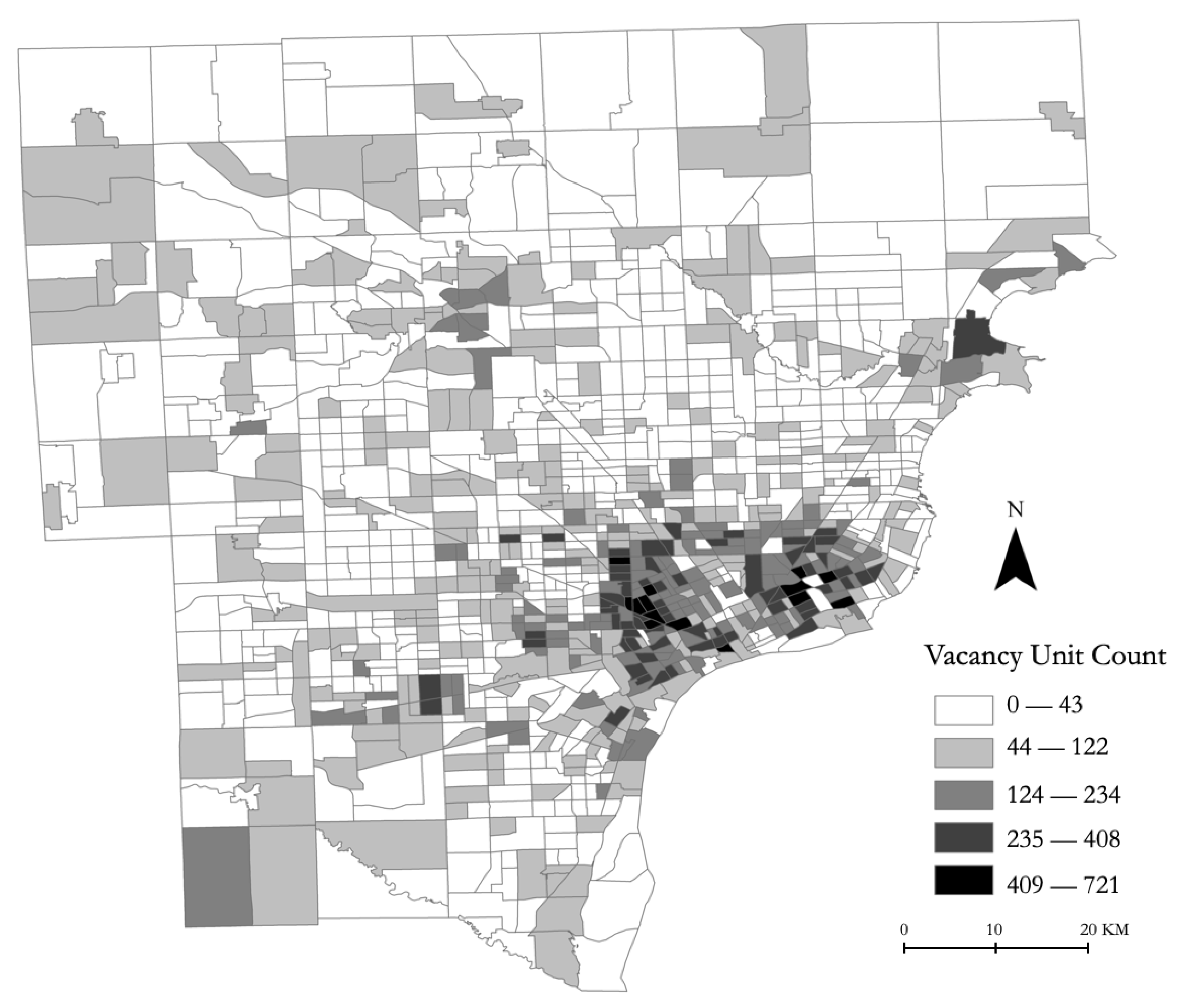
The city of Detroit is the largest city in Michigan, located in the Great Lakes area of the United States, which has also been given the moniker the “Rust Belt region”. There are many stories that discuss the greatness of this city during the 1950s—when the automobile manufacturing sector rapidly expanded and its population reached its peak [17]. However, the stories today often describe how over the last 60 years the city of Detroit has declined and shrunk. Specifically, how a growing city can rapidly become a declining one if it is focused on only one branch of economic production (e.g., in the case of Detroit this was the automobile). We believe that the city of Detroit is an excellent example of urban shrinkage. Numerous factors contributed to the bankruptcy of the city in 2013. One key reason is the increasing competition in the automobile manufacturing industry brought by globalization. Jobs in manufacturing tend to be more suburbanized and thus employment is more decentralized. Deindustrialization swept through the city of Detroit and its surrounding regions over the last few decades [18]. Another significant phenomenon that Detroit has witnessed is population loss, a decrease of over 60% in the last 60 years and 25% in the 10 years up to the 2010 census [5]. This process has accelerated the contraction of the housing market as employees in certain industries (e.g., manufacturing) become unemployed and seek employment elsewhere which results in more houses in residential areas becoming vacant. Large numbers of vacant properties and vacant land are now dispersed to almost every corner of the city. This is shown in Figure 1, where the darker color indicates more vacant units within each census tract from the 2010 census [19]. There were approximately 60,000 vacant parcels of land and about 78,000 vacant structures, of which 38,000 were considered to be unliveable in 2014 due to the potential for structural collapse [17]. With the increasing number of unliveable properties within the city boundary, the supply side of the housing market shrinks. In addition, population loss, caused by deindustrialization, and suburbanization lead to shrinkage on the demand side (i.e., people looking for homes). This combination of factors leads to the housing market shrinking from both the demand and supply sides in Detroit [20].

Figure 1.
Vacancy Unit Numbers of each Census Tract in Detroit Tri-County Area for 2010.
2.2. Literature Review
This section discusses the rationale for exploring urban shrinkage via dynamic computational approaches (unlike more static aggregate ones such as spatial interaction models); moreover, why we utilized an agent-based modeling approach by introducing works related to the topic of land markets (which, as noted above, are one of the main factors of urban shrinkage). However, before we discuss these, let us first present our rationale for choosing computational approaches. Our reasoning for this approach is that they allow us to test various scenarios and experiments in the safe environment of a computer. What we mean by this, is that it might not be feasible or ethical to carry out real world experiments, for instance setting a building on fire and watching how people might evacuate, but one can simulate such experiments in an computational model and observe the outcomes [21]. Generally speaking, such dynamical computational models fall within either the cellular automata or agent-based modeling methodologies [22]. Such modeling methodologies have been used to explore a wide-range of topics under the umbrella of urban dynamics (see for example: [23,24]). One of the most widely explored areas with such models is that of land use change and urban sprawl [25]. For example, the SLEUTH [26] model has successfully simulated land use transitions relating to the urban sprawl around the world (e.g., San Francisco, Washington, D.C.-Baltimore area, and “Chongqing, China, etc.) [27,28]. Recently, cellular automata models equipped with more advanced machine learning methods (e.g., Neural network and Random Forest) have been utilized to simulate urban expansion in China with enhanced accuracy over more traditional cellular automata approaches [29,30]. A closely related but slightly different approach to exploring land use change regarding urban sprawl is that of agent-based modeling. The major difference between agent-based modeling and cellular automata is that in agent-based models, one represents heterogeneous agents and each agent can have their own rule set which is generally not the case for cellular automata models where transition rules tend to be homogeneous [21,31,32,33]. By utilizing agent-based modeling, a variety of urban issues have been explored, ranging from urban growth [34], land use and land cover change [35], the rise of creative cities [36], to that of urban migration [37]. Focusing more on residential dynamics, agent-based models have been used to explore residential choices and gentrification (e.g., [38,39,40]). However, as noted by Schwarz et al. [41], there is a gap in simulating urban shrinkage through agent-based modeling.
Readers might be wondering why one might want to utilize agent-based modeling for examining urban shrinkage? One reason is the ability of agent-based models to capture the hierarchical structure of systems from the bottom-up, in a sense they focus on individual interactions of entities (e.g., individuals buying and selling houses) at the micro-level and allow us to capture more emergent phenomena at the macro-level (e.g., land markets). As such, agent-based models can provide insights into the target phenomenon or system of interest, especially for complex systems that involve human–environmental interactions [42,43]. In such systems, humans can impact the environment by their actions and in turn the environment can impact humans (e.g., [42]). Housing and land markets are excellent examples of human–environmental systems, as the main components in such markets at the micro-level are the buyers and sellers [44]. Such actors (i.e., agents) make their own decisions to trade or interact with each other and are impacted by the environment (e.g., economic and physical conditions) which can lead to a variety of housing market dynamics emerging overtime at the macro-level.
Secondly, agent-based modeling, unlike other modeling techniques, allows us to represent individuals as autonomous heterogeneous entities, each with different attributes (e.g., income), which make decisions based on what they know about other agents as well as the environment in which they are located [31,45]. With respect to housing and land markets, this is an important consideration as all actors in the system (e.g., the buyers and sellers) have different socioeconomic backgrounds, housing preferences, along with different bid and ask-price strategies [44,46]. Therefore, through the implementation of an agent-based model these heterogeneous characteristics and unique behaviors can be represented and simulated.
With respect to modeling markets, Gode and Sunder [47] were among the first to demonstrate how agent-based models could be utilized to capture supply and demand. In their abstract model, traders were selected at random to buy and sell goods and through these interactions demonstrated how supply and demand curves observed in “real” world situations could emerge through simulation. Turning to land markets, Filatova et al. [48] demonstrated how heterogenous agents with different ask and bid pricing behaviors could generate a land market in a stylized abstract environment while at the same time capturing urban growth, which was validated against Alonso’s [49] theory of land rent within a monocentric city. Other researchers have also explored land markets emerging from the bottom-up and how they impact land use within cities (e.g., [40,46]). For example, Torrens and Nara [40] simulated the demand and supply sides of a land market to explore urban gentrification in an area of Salt Lake City, Utah. However, while agent-based modeling of residential housing choices and land markets has started to show its potential as a valuable methodology for exploring urban issues from the bottom-up, no studies have examined land markets and urban shrinkage yet. Studies utilizing agent-based modeling to explore the urban shrinkage to date have mainly focused on land use and residential dynamics (e.g., [50]) instead of housing market dynamics.
We would argue that capturing housing markets is essential for understanding urban shrinkage, as the contraction of housing markets is caused by population loss under an urban shrinking situation [13]. Hence, a model of urban shrinkage should capture not only residential dynamics but also trades (or lack of) within the housing market. Therefore, an agent-based model stylized on spatially explicit data is presented in this paper to simulate the urban shrinkage in the Detroit Tri-County area. For the purpose of this model, we want to explore how micro-level housing trades impact on macro-level shrinkage by capturing trades between sellers and buyers within different dynamic sub-housing markets. Our initial efforts in this area were presented in [51], where we showed that a stylized model could not only simulate housing transactions but the aggregate market conditions relating to urban shrinkage (i.e., the contraction of housing markets). In this paper, we significantly extend our previous work by: (1) enlarging the study area; (2) introducing another type of agent, specifically a bank type agent; (3) enhancing the trade functions by incorporating agents’ preferences when it comes to buying a house; (4) adding additional household dynamics, such as employment status change. These changes will be discussed in more detail in Section 3, which we turn to next.
3. Methodology
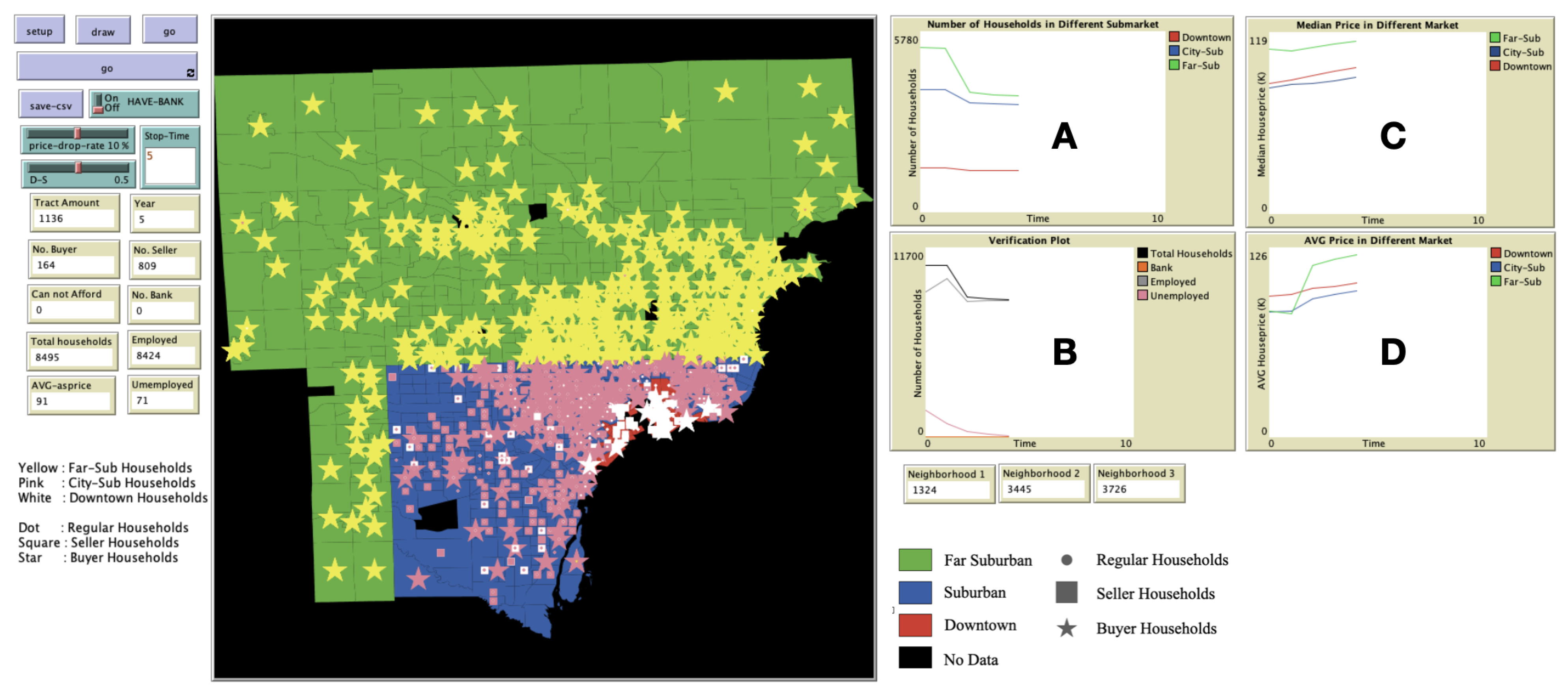
This section provides details utilizing the Overview, Design concepts and Details (ODD) protocol by Grimm et al. [52] for a model exploring urban shrinkage by simulating a generalized housing market based on the Detroit Tri-County Area, Michigan. In Section 3.1 we provide a brief overview of the study area and the agents in the model. Section 3.2 discusses model design concepts and Section 3.3 provides implementation details of the model. NetLogo 6.1 [53] was utilized to create the model. The model itself and a detailed ODD document [52] are available at: bit.ly/ExploreUrbanShrinkage, while the graphical interface is shown in Figure 2. We provide the model and data to allow readers not only to replicate the results presented in this paper but also to extend the model if they so desire.

Figure 2.
Model graphical user interface, including input parameters, monitors (left) and the study area (middle) and charts recording key model properties ((A): Number of households in different sub-markets; (B): Verification plot for total household numbers (e.g., total household number, number of bank agents, the number of employed and unemployed households); (C,D) show the median and average house price changes during the simulation).
3.1. Overview
3.1.1. State Variables and Scales
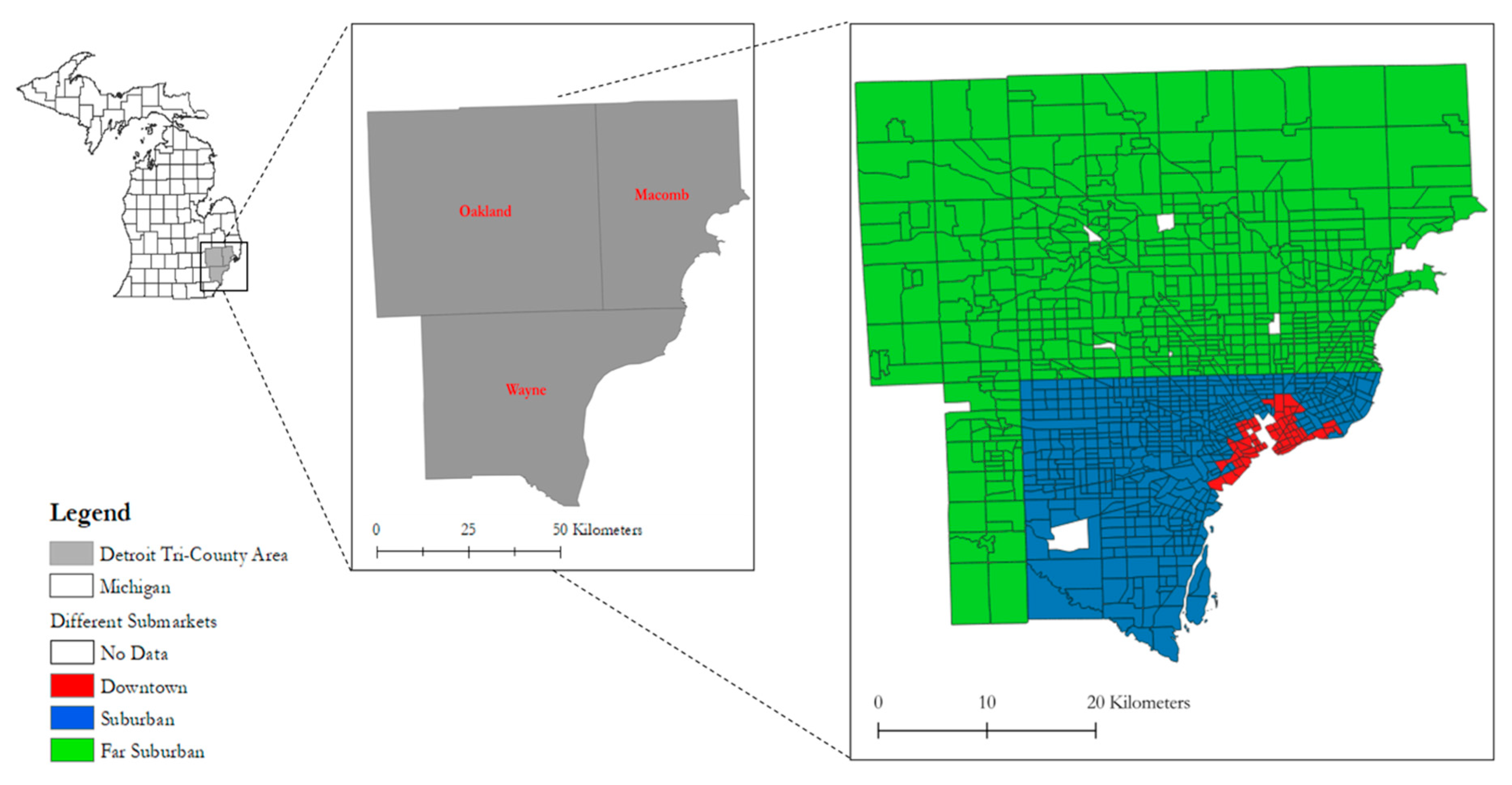
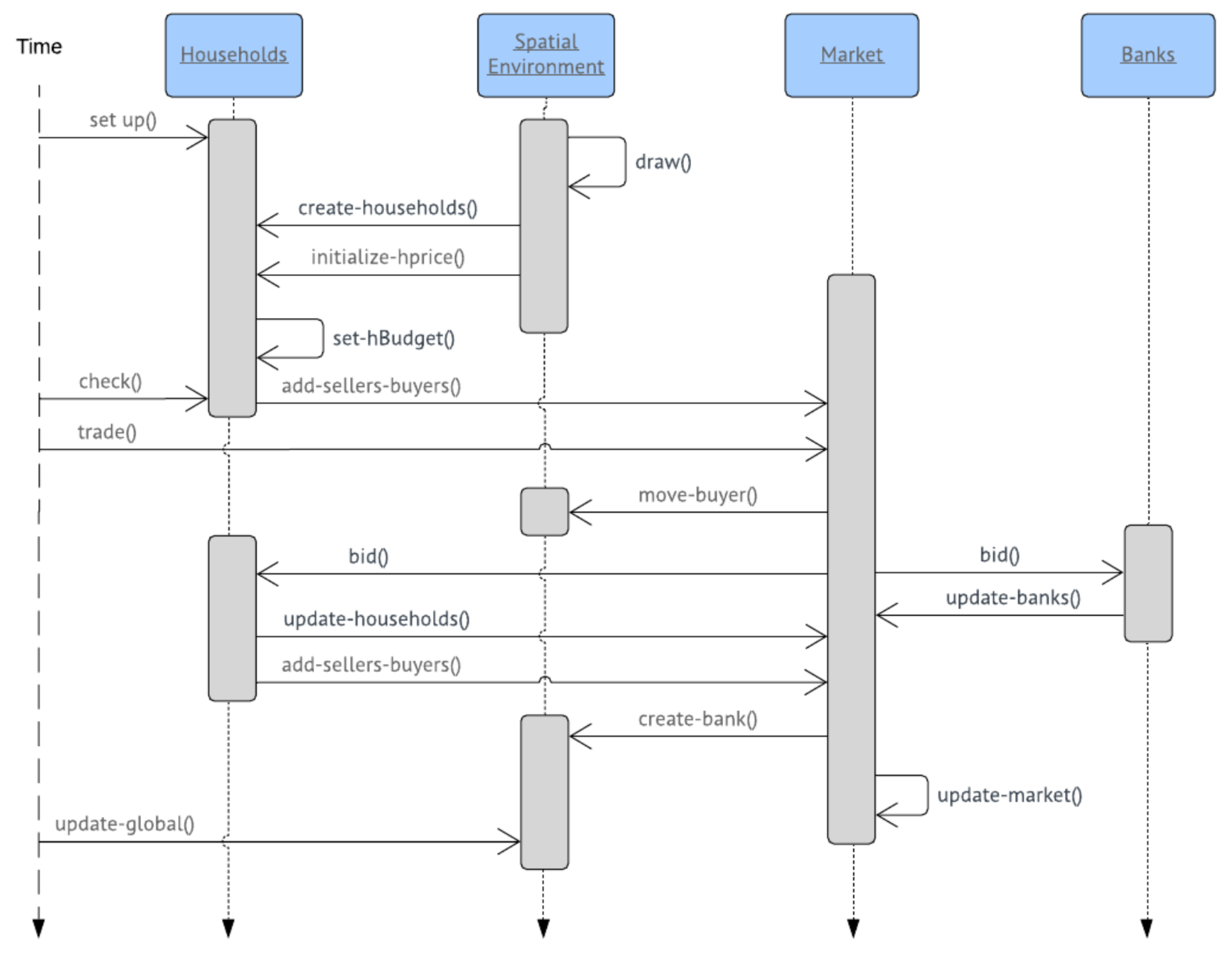
As noted in Section 2, the purpose of this model is to explore urban shrinkage by simulating housing transactions and the aggregate market conditions relating to urban shrinkage. Therefore, this model focuses on housing trades or transactions within various housing markets, rather than the economy as a whole. However, variables within the model that capture employment will be discussed in Section 3.4.2. Hence, trades between buyers and sellers within different sub-housing markets are simulated by this model. The whole Detroit Tri-County area can be divided into three sub-housing markets, which are comprised of: (1) downtown; (2) city suburban; and (3) far suburban housing markets, by utilizing spatial data which for an area of 5095 km as shown in Figure 3. Both the downtown area and suburban areas are within Wayne County. The difference is that the downtown area is defined by the Detroit opportunity zone data [54], while the city suburban areas exclude the downtown area. The rest of the study area, which we call far suburban, comprises part of Wayne County which is not defined as downtown or city suburban, along with Oakland and Macomb Counties, where the distance to the downtown area is much greater. In order to model, simulate and experiment with the housing market, we chose NetLogo as it has the capabilities to handle the spatial data needed to build the model and allows for rapid prototyping. The sequence of all the events in this model is displayed by the unified modeling language (UML) diagram in Figure 4, which demonstrates the model flow and dynamics.

Figure 3.
Study Area.

Figure 4.
Unified modeling language (UML) Diagram of the Model.
There are two types of agents in this model—households and banks. The main agents are households who live in the Detroit Tri-County area. In the model, for the purpose of simplification, one agent is used to represent 100 households. Agents are comprised of various attributes that result in a heterogenous population. Except for the attribute HPOLY, the rest of the agents’ attributes were selected for inclusion within the model based on relevant literature, which is summarized in Table 1. Agents are heterogenous and vary in their characteristics (e.g., ID, neighborhood type (i.e., HNT)) and finical backgrounds (i.e., HINCOME). Furthermore, household agents can be categorized into two types: buyers and sellers, and they are all goal-oriented. All buyers have one goal which is finding an affordable house by proposing a bid-price to sellers. If buyers are not able to find affordable properties in four consecutive years, they will be removed from the system. On the other hand, sellers aim to post an ask-price and maximize their profits from the trades (this will be further discussed in Section 3.4.1). Sellers who fail to sell their houses are forced to leave the system, at that time, the bank agent takes over the unsold houses and attempts to sell these houses. Further details about the role of banks is provided in Section 3.3.1. As for the attributes of the bank agents, only three attributes are inherited from sellers, which is summarized in Table 1.

Table 1.
Agent attributes.
The other component of this model is the environment, which contains two different elements: (1) Geo-spatial; (2) Artificial housing market comprising three different sub-markets—downtown, city suburban and far suburban. The geo-spatial environment provides a geographic boundary of the whole simulation area and the boundaries of the three sub-markets. Also, the geo-spatial environment provides a physical environment for all agents to move around and the places where the households are located. This environment also contains the artificial housing market, which captures the housing trades between buyers and sellers. The temporal scale in this model is one year, which is reflected by one time step in the NetLogo model. Every year, households make decisions to become buyers and to trade with sellers or banks. Our rationale for choosing a year is that it is unlikely for households to move more than once a year, and many other residential models use a 1 year time step (e.g., [34,38,50,56,57]).
3.1.2. Process Overview and Scheduling
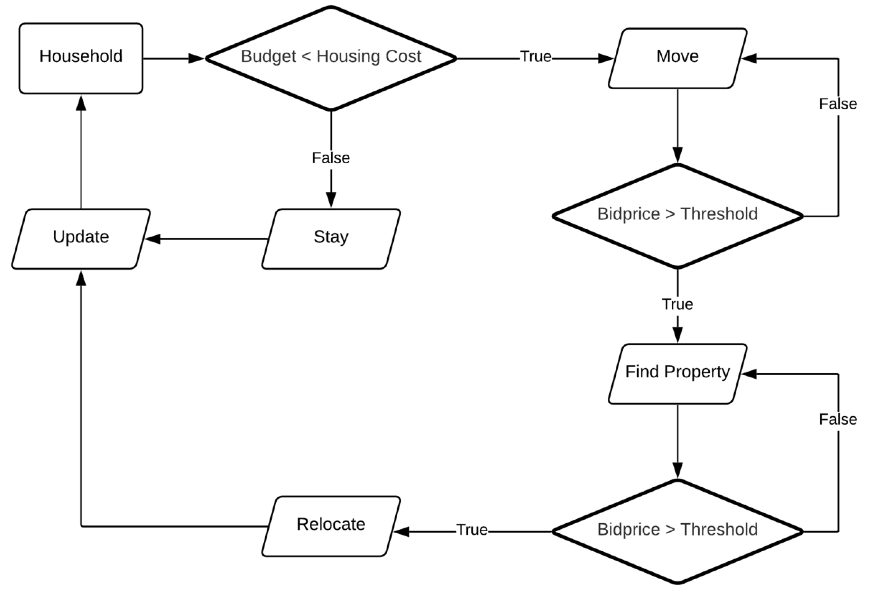
As discussed in Section 3.1, household and bank agents are the main entities in the model. The key attribute of the households is their income (i.e., HINCOME) level, which provides heterogeneity within the world and is updated as the simulation progresses (see Section 3.4.2). There are several models that have used income to control residential decision making (e.g., [48,49,55]). Accordingly, in this model, each household will make their decisions based on their income status, that is, to either stay or leave their current locations as shown by Figure 5. During each time step of the simulation, households will check if they can still afford their current living location based on their annual budget (i.e.,HBUDGET), which is calculated from their income. In addition, this income attribute also informs housing trades (i.e., what they can afford to buy). This affordability check will be explained in detail in Section 3.4.1. Once the buyer household decides to enter the housing market, they search for sellers (which include banks) to interact with based on their annual budget (i.e., HBUDGET). Similar to the real world, where buyers are restricted to what they can afford, buyers within the model choose sellers within the filtered list and offer a bid (i.e., a bid-price) to either sellers or banks, which will be discussed further in Section 3.2.1 and Section 3.4.1.

Figure 5.
Household Decision-Making Process for Stay or Leave Current Location.
3.2. Design Concepts
3.2.1. Observing
In order to capture the housing market dynamics, we measure various variables hierarchically, of which the details will be discussed in Section 3.5. At the macro-level, the overall average and median house price, as well as the total number of buyers and sellers within the study area is recorded at each time step of the simulation. At the micro-level, each different sub-market will capture the average and median house prices and the number of households through the entire simulation to reflect the differences among the three sub-markets in order to see if any shrinkage is occurring.
3.2.2. Sensing
All household and bank agents know which sub-markets they are located in and the price of the house they currently live in. As will be discussed in Section 3.4.1, they set budgets based on their own incomes and the budgets can be updated along with changes in income at each time step of the simulation. Housing trades are the main interaction in our model. Households who become buyers will use their budget to set the bid-prices (BIDPRICE). For buyers who fail to trade with sellers in one time step, the bid-price (BIDPRICE) will increase in the next time step. Each seller will set their ask-price (ASKPRICE) based on the current house price. The ask-prics (ASKPRICE) will decrease in the next time step if the seller fails to sell their current house. Banks have similar behavior to that of sellers. The only difference is that the bank decreases their ask-price at a greater rate. The rationale for this is because banks may want to sell the house within a short time frame [58]. Details related to bid-price and ask-price dynamics will be discussed in Section 3.4.2. Within the housing market, buyers make trades with sellers and they will know every seller’s ask-price, which allows buyers to choose a specific seller based on their financial capabilities. The trade will happen once the buyer finds a seller to trade with and they agree upon the price. Further discussions related to the negotiation process are provided in Section 3.4.1.
3.3. Details
3.3.1. Initialization
The initialization of the model is based on socioeconomic and geo-spatial data of the study area. The socioeconomic data (e.g., income, employment status, house prices) come from the Decennial Census [19] for each census tract in the study area. Before applying this data to initialize the number of household agents within our simulation, the data were preprocessed using Python to allow for efficient input into the NetLogo platform. Due to the computational constrains of NetLogo, simulations that entail a large number of agents are computationally intensive and time-consuming. To mitigate this we therefore only represent 1% (i.e., 10,602) of the total number of households within the study area. The model initializes the household agents tract by tract. There is a total of three stages during the initialization process: (1) Create households; (2) Assign employment status; (3) Assign house price. The households are initialized by using the income background from the census dataset. For instance, if 500 households fall into the $10,000 to $15,000 income range for a certain tract, five household agents will be generated with their incomes assigned to this range. As for the income, if the household agent is generated within the $10,000 to $15,000 income range, the income of this household will be ten plus a random integer between 5. After the generation of the households, several socioeconomic attributes are introduced to the household agents, such as employment status and house prices, which provides the household agents with more heterogeneous attributes. The employment status is extracted directly from the census dataset to assign each household agent an employment status. For instance, if 20% of the households are employed in a particular tract, the model will assign 20% of households in this tract as employed and the rest of them will be unemployed. To assign the house price for each household, the procedure is similar to assigning employment status. We use the percentage of households falling into various house value ranges to assign the house value. For instance, if 20% of households’ house values fall into $50,000 to $100,000, those households’ house values will be 50 plus a random integer within 50.
In addition, three input parameters are used to initialize the model. The first being the demand and supply condition (D-S parameter), which controls the ratio of buyers and sellers. The model generates sellers based on the number of buyers. For instance, when set to default (i.e., 0.5) the total number of buyers and sellers initialized is equal which indicates equal demand and supply. While 0.1 would reflect demand exceeding supply (i.e., more buyers than sellers), 0.9 would be the opposite (Section 4 shows the results of changing this parameter). The second input parameter, HAVE-BANK? allows the model to add a bank agent. When set to its default (i.e., True), the bank agent is added to the model (more details about the bank agent are given in Section 3.4.2). The last input parameter is Price-Drop-Rate, which was inspired by what we see in the real world; that when a house has been on the market for several months, the sellers often drop the price. A notable model that does something similar is that of O’Sullivan [39], which decreased the percentage for each seller’s ask-price in the next time step if the property remained unsold. Table 2 provides an overview of the model input parameters along with their default values.

Table 2.
Initialization parameters’ default values.
3.3.2. Inputs
Data play an important role in model parameterization, as discussed in Section 3.3.1, with respect to the initialization of the simulation. Furthermore, data play a role in validation which we will discuss in Section 4. Two categories of vector data are utilized in this work: spatial data and socioeconomic data. Spatial data include: (1) Detroit city boundary (shown in Figure 3); (2) Tri-County area boundary including Wayne County, Oakland County, and Macomb County; (3) All census tract boundaries for the Tri-County area. The census tract boundaries can be associated with socioeconomic data which were acquired from the census dataset [19], as shown in Table 3.

Table 3.
Census Variables for Model Initialization.
3.4. Sub Models
3.4.1. Housing Market
There are three stages for the simulation process: (1) affordability check of household; (2) generation of sellers and buyers; (3) trade and move-in. First, households will check their affordability on their current house by comparing their annual budget (i.e., HBUDGET) and the minimum housing cost (which we describe below). To check this, all households will set their budgets, which represents 34% of their income (i.e., HINCOME) and can be used on annual house fees, including property tax, annual maintenance, mortgage payments, and so forth [59]. To calculate the minimum housing cost, three percentage numbers are referenced including 1.52% of the house price for the property tax, 1.3% of the house price for the annual maintenance fee and 4.54% of the house price for mortgage payment [60,61,62]. Hence, we set 7.38 % of the house price as the minimum housing cost, which indicates the lowest annual cost for a house. If one household’s minimum housing cost exceeds the annual budget (i.e., HBUDGET), which indicates the household cannot afford their current house, they will enter the housing market. Secondly, the buyers and sellers will be generated based on demand and supply (D-S), which was discussed in Section 3.3.1.
As for the key interaction within the model, the trade (and subsequent moving in) process comprises two stages: (1) buyers find sellers; (2) a negotiation on the price. For the first stage of the trade, buyers will search for sellers (i.e., moving around the physical environment). Buyers are able to enter every sub-market; however, buyers may not enter the downtown sub-market first, due to perceived issues with neighborhood security which may have negative impacts on buyer’s households’ decisions when purchasing a new home [63]. Hence, we assume that properties in the downtown sub-market are less preferred compared to city suburban and far suburban. As such, a buyer may enter the far suburban sub-market first, and then search for sellers (i.e., homes for sale), because of the perceived notions of overall safety conditions and a better quality of life in the far suburban areas [63]. If a buyer is not able to find a seller in the far suburban sub-market, the buyer will enter the suburban sub-market and continue to search for sellers. Rather than exclude buyers from the downtown sub-market, a buyer may only enter the downtown sub-market if they cannot find any sellers in both far suburban and city suburban sub-markets. To determine whether the buyer can afford house or not, buyers have knowledge related to all of the sellers’ ask-prices, which is analogous to what we see when using a real estate website to search for a new home. The buyers will set the bid-price (i.e., BIDPRICE), which is 2.5 times their gross income [64]. When a buyer searches for a new location, they keep checking the ask-prices (i.e., ASKPRICE) of the sellers located in that area. Buyers will then sort out a list of sellers based on their initial bid-prices (i.e., BIDPRICE) when they move to a new area. For example, sellers with ask-prices less than 1.1 times that of a certain buyer’s bid-price and greater than that buyer’s bid-price may be sorted into the list. If there is only one seller in a specific area, the buyer will only bid on one house in one time step. However, if there are more sellers in a specific area, the buyer’s bid-price may be reviewed by all those sellers located in the same area, which can be considered multiple bids in the same area in one time step (hence buyers can make multiple offers in one time step). After this stage, the sellers attempt to complete a trade. The sellers’ goal is to maximize their profit from the trade, so they will choose the buyer with the best bid-price. After the trade is completed, the trade will be recorded.
3.4.2. Households and Banks Dynamics
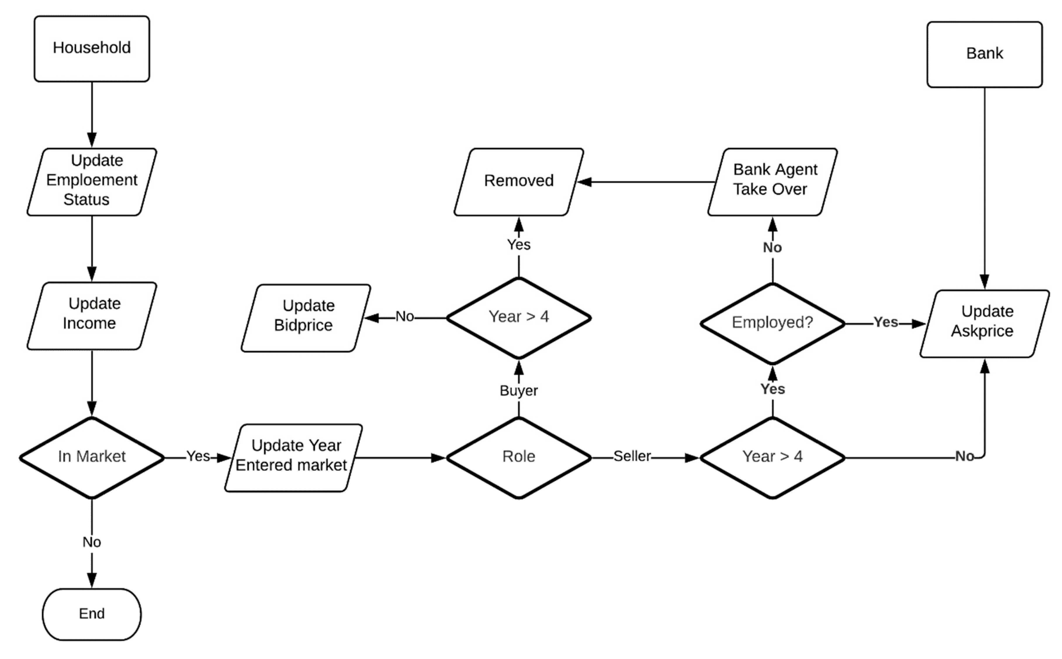
To imitate reality, several dynamics are introduced to the household and bank agents. The process is shown in Figure 6. For all households, employment status (EMPLOYED?) may change each time step, which is inspired by Patel et al. [55]. For example, employed households have a certain probability to lose their job; similarly, unemployed households may have the probability of finding a job. As shown by Equation (1), the incomes’ dynamics are based on the employment status of the agents. is the income at time , is the income at time t and represents the employment status. If one household has a job, will be the 0.5, if not, it will be −0.1. The employment status therefore impacts the households’ income (HINCOME), which has a direct influence on their annual housing budget.
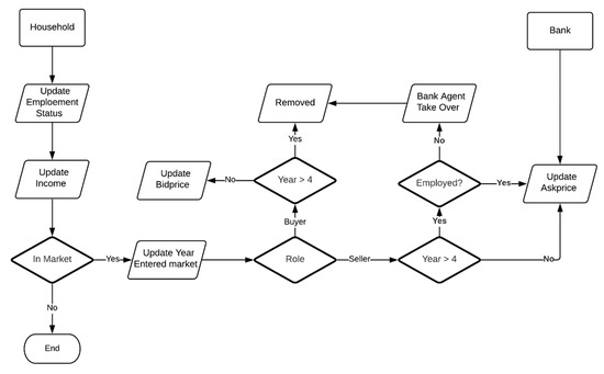
Figure 6.
Household Dynamics.
Population dynamics are reflected both by the sellers and buyers. As for sellers, if they are employed but are unable to sell their houses over four consecutive years (i.e., time steps), they may stay and keep trying to sell the house until a buyer is found. While, for sellers who are unemployed, if they cannot sell the house in four consecutive years, they will be removed from the system (akin to foreclosure). At that time, the bank agent may take over their houses and keep trying to sell it. From the buyer’s side, if they are unable to find a house to purchase in four consecutive years, they will be removed from the system. This dynamic indicates that those buyers who cannot afford a house in any of the sub-markets based on their financial status may move out from our study area to somewhere else. Also, the dynamics of bid- and ask-prices are added to the model. From the seller side, the ask-price (ASKPRICE) may decrease when the house is not sold [39]. For example, in the model, if a seller or a bank fails to sell a house, the ask-price will decrease based on the Price-Drop-Rate in the next time step, which is shown in Equation (2). is the ask-price at time , is the ask-price at time t and PDR represents Price-Drop-Rate. The bank agent’s ask-price drop rate is doubled compared to that of a seller household. This is to reflect the banks wishing to clear their inventory and recoup money owed as fast as possible.
As for the buyers, the bid-prices (i.e., BIDPRICE) are impacted by their income (i.e., HINCOME). Other than that, buyers who fail to find a seller or bank to trade with may increase their bid-price based on their budget (i.e., HBUDGET) as shown in Equation (3). is the bid-price at time , is the bid-price at time t and is the random number generated based on how much percentage a buyers bid-price can exceed their initial offer. In our model we use 0.1, which indicates a buyers’ bid-price may not exceed %110 of initial bid-price. This concept is based loosely on land market models (e.g., [46,48]) where buyers have a willingness to pay up to a certain percentage point over their initial bid-price.
3.4.3. Economic Environment
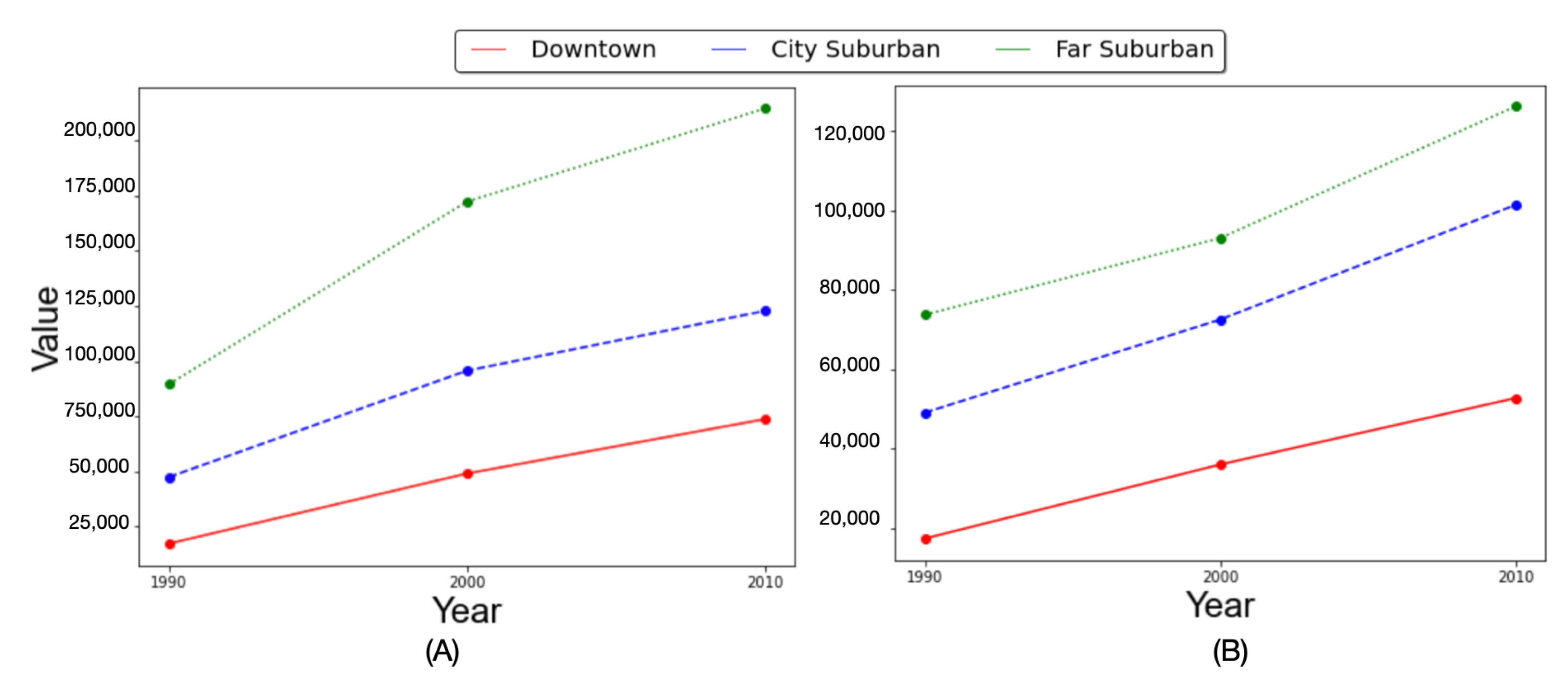
The economic environment is the invisible hand in the model and takes into account inflation of house prices, which imitates economic inflation. Although the trend of the economy in Detroit has been downwards, for example, there are few extreme cases where homes have been sold for $1 [65]. According to 1990, 2000, and 2010 census data, the overall house prices show an upward trend as seen in Figure 7A. The median house prices are all increasing. One reason for this relates to general inflation. However, when disregarding the impact of inflation by using the United States inflation calculator [66], the house prices still keep increasing over time, as shown in Figure 7B. Hence, in the model, house prices will increase during the simulation based on annual inflation rates taken from [66].
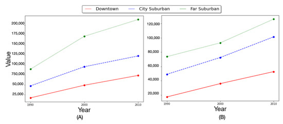
Figure 7.
Census Data on Median House Prices from 1990, 2000 and 2010 (A) Median House Price, (B) Median House Price without Inflation.
3.5. Model Outputs
In Section 1, the contraction of the housing market and population loss are the consequences of urban shrinkage, which is what we want to explore with this model (as discussed in Section 2 and Section 3). In order to explore this, a range of outputs are generated by the model. To explain the urban shrinkage, we specifically focus on the changes on the number of households and the changes in house prices within different sub-markets. As discussed in Section 3.4.1, these selected outputs are the result of the housing trades in the model. To capture the changes in house prices, median and average house prices of each sub-market are used to reflect the price dynamics. At the same time, median and average house prices for each census tract are also recorded by the model to show the spatial disparity of the house prices.
4. Results
Before detailing the results of the model, we first want to discuss our efforts for verification. Here we refer to verification as the process of checking if the model matches its design [45]. In this study, verification of the model was performed by conducting code walkthroughs, visual debugging [67] and a series of control variates experiments to ensure the model was working as designed [68]. These tests ensured that we made no logical errors in the translation of the model into code, and that there were no programming errors. Visual debugging can be carried via the model interface when the model is running. Figure 2 not only introduces the model interface, but also shows an example of visual debugging during a model run. For individual households, we use various shapes and sizes to distinguish different roles and status during a simulation. For example, a dot represents a regular household, a square represents a seller household and a star represents a buyer household, and the size differences of stars indicate the difference statuses of buyers during the trade. A larger star represents a buyer who has successfully completed a house purchase. Other than visual verification at the micro-level as discussed above, four plots (e.g., plot A, B, C, D) are used for macro-level visual verification as shown in Figure 2. Plot A captures the change in the number of households during the simulation. Plot B outputs some generic results (e.g., total household number, number of bank agents), but the main purpose of this plot is to show that the households’ employment statuses are updating (i.e., changing) over the simulation, which was discussed in Section 3.4.2. As for Plots C and D, they show the median and average house prices during the simulation. With these plots updating during the simulation, we can ensure that the model does not have programming errors that stop the simulation instantly, but further experiments were needed to test the impacts of the input parameters, which it is not possible to capture through visual debugging alone and we turn to this next.
As discussed in Section 3.3.1, three input parameters were used in the model: (1) D-S; (2) HAVE-BANK?; (3) Price-Drop-Rate. To test these three input parameters, a series of control experiments were carried out for verification purposes. For instance, when verifying D-S, we only modified the value of D-S and kept the other two parameters set to default values as shown in Table 2. Each experiment was run 50 times and, in what follows, we describe only the average results.
To verify D-S (see Section 3.3.1), one does not need to run the model, as D-S is only used when the model is being initialized to set the number of buyers and sellers. Therefore we tested various D-S values (e.g., 0.1, 0.5 and 0.9) and noted its outcome with respect to number of buyers and sellers. Various D-S values stand for different demand and supply scenarios, which will be discussed further below. As shown in Table 4, the model is able to generate different numbers of buyers and sellers by modifying the value of D-S. As for the other two parameters (i.e., price-drop-rate and HAVE-BANK?), because they are used during the simulation, the following verification experiments were undertaken.

Table 4.
Verification of D-S.
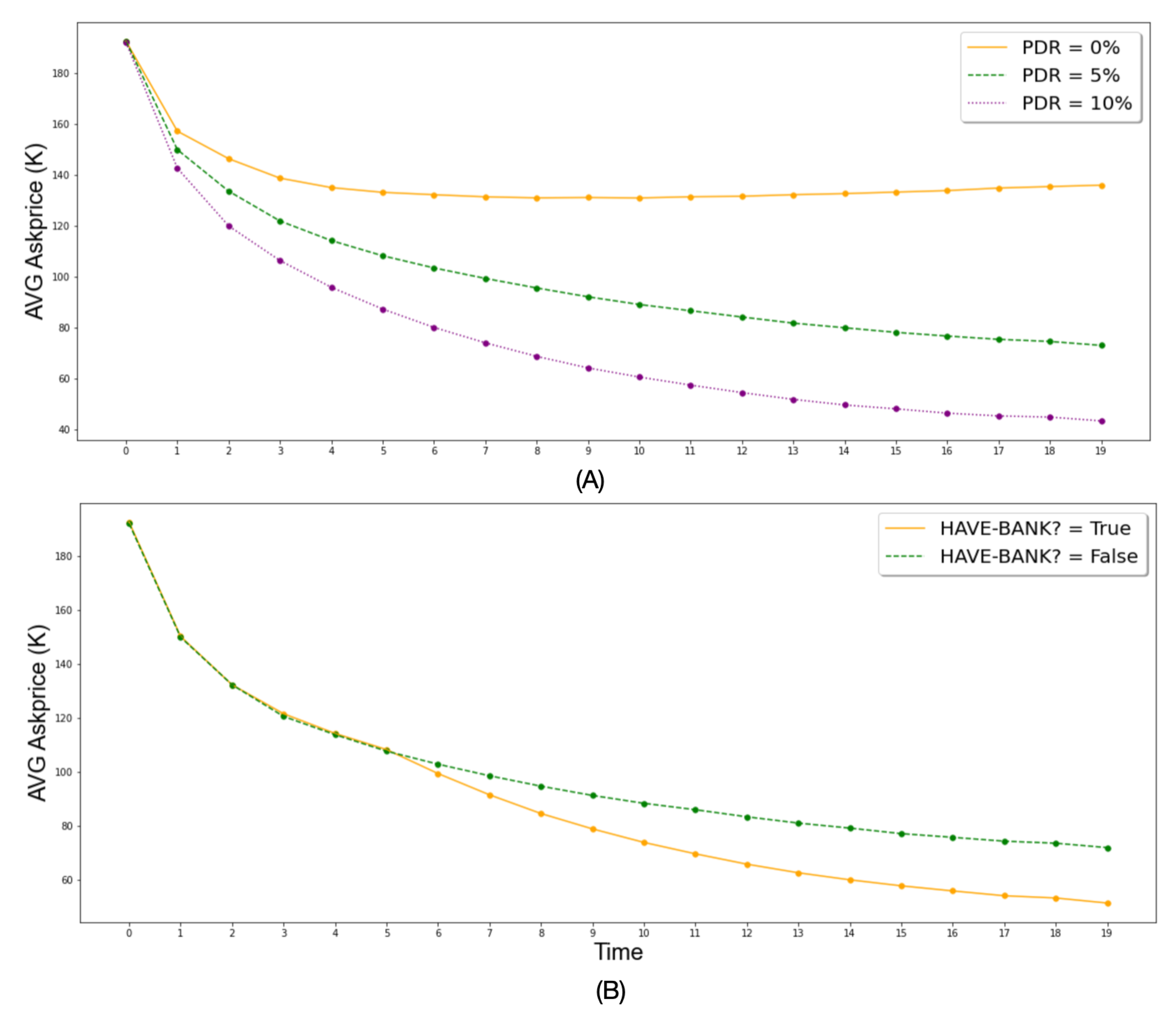
To test price-drop-rate, we carried a series of extreme value tests by setting the parameter to 0, 5, and 10 which represents how much of a percentage of the ask-price will be decreased in each time step if the house is not sold. In this experiment, the bank agent is not added (i.e., HAVE-BANK is False), our rationale for this is that the purpose here is simply to test the impacts of Price-Drop-Rate on ask-price. Hence, by capturing the average ask-price changes over the course of a simulation one gains sufficient evidence for this stage of verification. As Figure 8A shows, when increasing the value of Price-Drop-Rate, the average ask-price decreases more, which indicates that the Price-Drop-Rate parameter does have an impact on the average ask-price and this parameter works as intended.
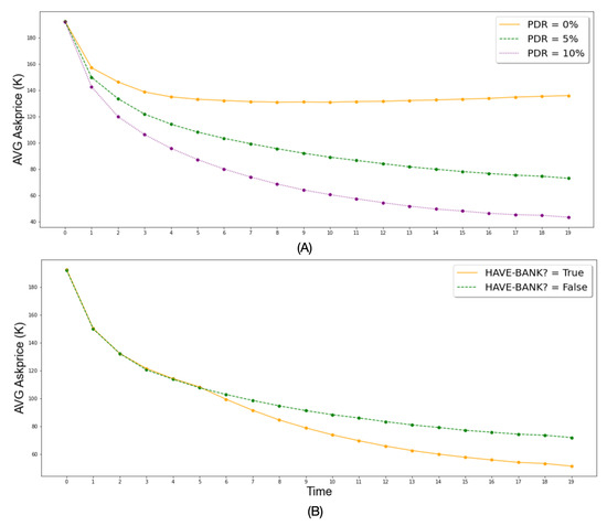
Figure 8.
Average Ask-price Changes with Different values of Different PDR (A) and HAVE-BANK? (B).
Moving to the verification of HAVE-BANK?, as discussed in Section 3.3.1, HAVE-BANK? allows the model to add a bank agent. Unlike that of regular sellers, bank agents’ ask-price drop rate is doubled (seen Section 3.4.2). Hence, we assume that with the increasing number of bank owned properties, the average ask-prices may decrease more than those in a scenario where there is no bank agent. In Table 5, we capture 805 bank owned proprieties by the end of the simulation, which indicates HAVE-BANK? is capable of adding a bank agent when the need arises. Figure 8B shows that the average ask-price drops with the increasing number of properties owned by the bank agent, and the average ask-price is lower compared to the no bank scenario. This suggests that the bank agent is added properly by the model. After carrying out these tests, we feel confident that the model behaves as it is intended and matches its design and thus is verified.

Table 5.
Verification of Input Parameter.
Now, turning to model results and validation, we refer to validation as the process ensuring the model aligns to the real world, specifically how the model can capture basic market behavior as it potentially relates to urban shrinkage. In order to do this we present three simulation scenarios of different demand and supply conditions for a period of 20 (year) time steps. We ran each scenario 50 times and, in what follows, we describe only the average results. We chose 20 years as this will cover the years of 1990, 2000 and 2010, which we have census data for, which in turn can be used to validate the model. To control for demand and supply, we only changed the D-S parameter in the model and kept all other parameters at their default values (e.g., Table 2). Three different scenarios were simulated to explore how different demand and supply conditions impact on median and average house prices in the different sub-markets: (1) equal demand and supply; (2) demand exceeds supply; (3) supply exceeds demand. Table 6 shows the final median and average house prices in each sub-market for different D-S settings, which are the same values described in Section 4.

Table 6.
Median and Average House prices (K) in Different sub-markets at the End of the Simulation.
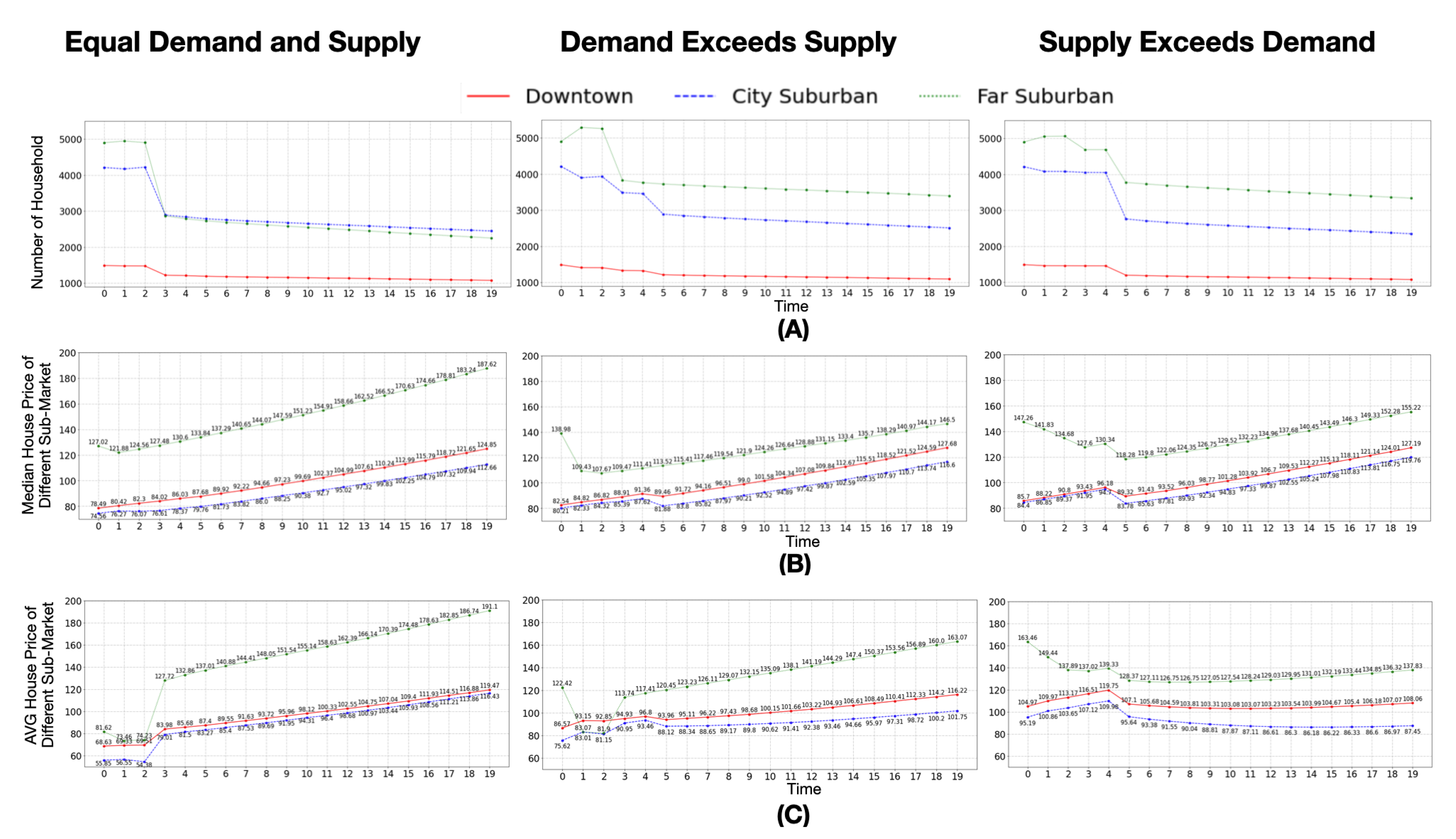
Building on Table 6, Figure 9A shows the three scenarios with respect to the number of households in each sub-market. As Figure 9A shows, the overall trend of household numbers in all the three scenarios are decreasing, which can be considered as population loss in a shrinking city. However, one can see that around time step 5, there is a drop in the number of households. This drop is due to the bank agent entering the simulation and taking over sellers’ houses which were unsold (as discussed in Section 3.4.2). Figure 9B,C demonstrates how median and average house prices change over the simulation scenarios. The results indicate that among all three simulation scenarios, the median and average house prices in different sub-markets turn out to be increasing. This is due to inflation, which is included in our model (as discussed in Section 3.4.3). The simulated increasing house price trends are similar to those of the empirical data which was shown in Figure 9.
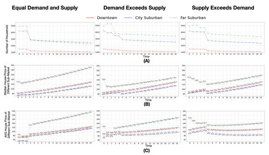
Figure 9.
Validation on Market Behaviors, Number of Household (A), Median (B) and Average (C) House Prices Change in Different Demand and Supply Scenarios.
If the demand exceeds supply scenarios, although all buyers are attempting to find sellers and complete trades (i.e., buy a house), due to insufficient sellers generated at initialization of the model, the number of relocating households is the lowest among all scenarios. However, as shown in Table 6, the model captures the highest median house price in the far suburban sub-market (which is approximately 60% more than that of downtown), which is due to the sellers flooding this area as discussed in Section 3.4.1 and is similar to what one sees in the “real world” (i.e., Figure 7). This suggests the model captures the correct market behavior.
While in the demand equals supply scenario, due to a relatively balanced market, we witness the most household relocations being captured, along with lowest median house prices in suburban and far suburban sub-markets (i.e., suburban: 116.60; far suburban: 146.50). However, the median house price in the downtown sub-market is not the lowest among all scenarios (i.e., 127.68). This result might sound counter-intuitive because one would expect the lowest median house price in the supply exceeds demand scenario, however, the average house price for all three sub-markets in this scenario is in the middle of all the scenarios which suggests there are nuances in how one should record and report the results of the model. One reason for this result could be because all buyers have preferences for purchasing houses in far suburban and suburban (as discussed in Section 3.4.1), which leads to a relatively competitive market. In addition, all sub-markets’ average house prices are the lowest among all scenarios.
By discussing the results above from the three scenarios, hopefully it is clear to the reader that our model captures urban shrinkage from the aspect of decreasing numbers of households in the downtown sub-market. Also, similar to empirical data as shown in Figure 7, even without inflation, house prices are still increasing even in a well-known shrinking city and our model captures similar trends in the three scenarios (as shown in Figure 9). To some extent one could consider such results as level 2 validation in terms of the Axtell and Epstein [69] schema of classification of model validation, in the sense we can attain quantitative agreements of emerging macro-structures (e.g., declining number of households and increasing house prices) from the bottom-up. We illustrate this in Figure 10 which shows the resulting house prices from the demand equals supply scenario. More specifically, Figure 10A illustrates a heat map of each census tract’s median house price at the end of the simulation, while Figure 10B displays the heat map of the average house price. According to these heat maps, high median and average house prices are mainly captured in far suburban sub-markets.
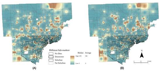
Figure 10.
Heat Maps of Median (A) and Average (B) House Prices at the End of the Simulation where Demand equals Supply.
5. Conclusions and Discussion
While we are witnessing a global growth of the urban population, which raises concerns about urban sustainability (e.g., [9,70,71]), not all cities are growing (Section 1). Some, like Detroit, are actually shrinking, which has drawn a lot of discussion from the research and practice communities globally as it causes population loss, economic decline and a growth in crime due to vacant properties and housing market contraction (e.g., [7,13,14,72]). However, few efforts have been made to explore this phenomenon from a modeling and simulation domain. This paper significantly adds to this nascent field of inquiry by specifically capturing how the buying and selling of houses can lead to urban shrinkage from the bottom-up through a case study of the Detroit Tri-County area. Results from this model (i.e., Section 4) have implications concerning urban shrinkage. For example, we show how household decline in an area could potentially lead to less tax revenue and therefore limits a city’s ability to provide services, which in turn can lead to more urban decline as discussed in Section 1. Although the simulated median and average house prices are showing an upward trend, which seems inconsistent with the intuitive results of a contracting housing market (i.e., the decreasing of house prices), this was due to the inflation over the simulated years (see Section 3.4.3 and Section 4).
While our model can capture urban shrinkage, like all models there are limitations and there is always room for improvement. One area of improvement could be to extend the model to represent more types of housing stock (e.g., apartments, single family homes, etc.) which could be sourced from the American Community Survey or local government property records along with home sales data. We chose not to go this route here as the purpose of the model was to act as a prototype to explore how urban shrinkage might emerge from the bottom-up through the interactions of buying and selling houses. Another area of further work could be to better characterize new incoming populations. In the current model we did not introduce new households based on their heterogeneous financial and demographic backgrounds due to data limitations (i.e., the census data is not continuous between 2000 and 2010). As a result of this, the final simulated household numbers may be lower than the empirical data. With this being said, the declining trend in the number of households for the whole study area is captured successfully by the model, which aligns with the empirical data. One way to better capture new households entering the study area is to use techniques from synthetic population generation such as those seen in dynamic micro-simulation models (e.g., [73]). This would potentially allow us to better capture how changes in demographics impact on residents’ ability to stay in an area and their preferences for certain types of neighborhoods, but that is beyond the scope of this current paper as this would be a large undertaking and most agent-based models like the ones cited in Section 2 only look at one aspect (i.e., subsystem) such as the land market rather than the entire urban system itself [45].
Building upon this idea, the model presented in this paper only explored the buying and selling of properties; however, as we noted in the introduction (Section 1), urban shrinkage is a complex issue and we do not specifically model the economic environment comprehensively (rather we simply consider inflation as only an aspect of the economic environment). This simulation could be improved by incorporating time series data with respect to the economy such as unemployment rates or economic growth. Alternatively one could couple this model with a more macro economic model to account for such factors (e.g., [74,75]). Other than incorporating more data into the simulation, the model could capture more nuanced residential dynamics if the time step was deceased from a year to, say, monthly. This would allow for a slower incremental price dropping of house values if they remained unsold. It would also be interesting to experiment with multiple space-time scales in order to explore the equifinality of urban shrinkage at different temporal and spatial scales (e.g., [76]). Another area of work, especially with respect to urban sustainability, would be to explore what it would take to stop urban shrinkage, or how neighborhoods go from declining to growing, such as through gentrification. Gentrification in Detroit has been discussed in the literature (e.g., [77,78,79]). Hence, another direction to extend the model would be to explore gentrification in Detroit through modeling and simulation. Similar to urban shrinkage, there is a growing body of models (e.g., [39,40,80]) that show promise for capturing such phenomena. Moving the focus point from Detroit to other metropolitan areas, we believe the model presented here could be generalized across metropolitan areas by integrating more data and adding new types of agents (e.g., investors whose behaviors are different from households and banks). This is one reason we provide the code and the data to the model (see Section 3), to allow other researchers to extend and explore the model as they see fit. Even with these limitations and areas of further work we believe this paper has demonstrated how agent-based modeling integrated with geo-spatial data provides a promising method for exploring urban shrinkage and, if developed further, potentially offers a means to test policies to alleviate this issue.
Author Contributions
The genesis of this work stems from Y.X. who also provided the data. N.J. and A.C. conceptualised the model and experiments. N.J. coded the model and ran the simulations, who along with W.W. carried out the analysis and wrote up the results. Both A.C. and N.J. prepared the initial draft while W.W. and Y.X. provided substantial edits to the paper and all authors approved its content. All authors have read and agreed to the published version of the manuscript.
Funding
This research received no external funding.
Institutional Review Board Statement
Not applicable.
Informed Consent Statement
Not applicable.
Data Availability Statement
The data and model presented in this study is openly available at: www.comses.net/codebases/dd834a64-34b8-43a3-b27b-9876a848ffdb/releases/1.0.0/.
Acknowledgments
The authors would like to thank the Center for Social Complexity at George Mason University, the RENEW Institute at the University of Buffalo and Institute of Geospatial Research and Education at Eastern Michigan University for providing opportunities that enabled this work.
Conflicts of Interest
The authors declare no conflict of interest.
Abbreviations
The following abbreviations are used in this manuscript:
| ABM | Agent-based Modeling |
| CA | Cellular automata |
| ODD | Overview, Design concepts and Details Protocol |
| UML | Unified Modeling Language |
References
- United Nations. 2018 Revision of World Urbanization Prospects. Available online: https://population.un.org/wup/ (accessed on 3 February 2020).
- Wei, Y.D.; Li, H.; Yue, W. Urban Land Expansion and Regional Inequality in Transitional China. Landsc. Urban Plan. 2017, 163, 17–31. [Google Scholar] [CrossRef]
- Haase, D.; Lautenbach, S.; Seppelt, R. Modeling and Simulating Residential Mobility in a Shrinking City using an Agent-based Approach. Environ. Model. Softw. 2010, 25, 1225–1240. [Google Scholar] [CrossRef]
- Long, Y.; Wu, K. Shrinking Cities in a Rapidly Urbanizing China. Environ. Plan. Econ. Space 2016, 48, 220–222. [Google Scholar] [CrossRef]
- Neill, W.J.V. Carry on Shrinking?: The Bankruptcy of Urban Policy in Detroit. Plan. Pract. Res. 2015, 30, 1–14. [Google Scholar] [CrossRef]
- Couch, C.; Karecha, J.; Nuissl, H.; Rink, D. Decline and Sprawl: An Evolving Type of Urban Development–Observed in Liverpool and Leipzig. Eur. Plan. Stud. 2005, 13, 117–136. [Google Scholar] [CrossRef]
- Großmann, K.; Bontje, M.; Haase, A.; Mykhnenko, V. Shrinking Cities: Notes for the Further Research Agenda. Cities 2013, 35, 221–225. [Google Scholar] [CrossRef]
- Reckien, D.; Martinez-Fernandez, C. Why Do Cities Shrink? Eur. Plan. Stud. 2011, 19, 1375–1397. [Google Scholar] [CrossRef]
- Slach, O.; Bosák, V.; Krtička, L.; Nováček, A.; Rumpel, P. Urban Shrinkage and Sustainability: Assessing the Nexus between Population Density, Urban Structures and Urban Sustainability. Sustainability 2019, 11, 4142. [Google Scholar] [CrossRef]
- Bontje, M. Facing the Challenge of Shrinking Cities in East Germany: The Case of Leipzig. GeoJournal 2004, 61, 13–21. [Google Scholar] [CrossRef]
- Deng, C.; Ma, J. Viewing Urban Decay from the Sky: A Multi-scale Analysis of Residential Vacancy in a Shrinking US City. Landsc. Urban Plan. 2015, 141, 88–99. [Google Scholar] [CrossRef]
- Shane, J.M. Abandoned Buildings and Lots; U.S. Dept. of Justice, Office of Community Oriented Policing Services: Washington, DC, USA, 2012.
- Martinez-Fernandez, C.; Audirac, I.; Fol, S.; Cunningham-Sabot, E. Shrinking Cities: Urban Challenges of Globalization. Int. J. Urban Reg. Res. 2012, 36, 213–225. [Google Scholar] [CrossRef]
- Xie, Y.; Gong, H.; Lan, H.; Zeng, S. Examining Shrinking City of Detroit in the Context of Socio-spatial Inequalities. Landsc. Urban Plan. 2018, 177, 350–361. [Google Scholar] [CrossRef]
- Kneebone, E. Job Sprawl Stalls: The Great Recession and Metropolitan Employment Location. 2013. Available online: https://www.brookings.edu/research/job-sprawl-stalls-the-great-recession-and-metropolitan-employment-location/ (accessed on 7 February 2021).
- Kneebone, E. The Changing Geography of US Poverty. 2017. Available online: https://www.brookings.edu/testimonies/the-changing-geography-of-us-poverty/ (accessed on 7 February 2021).
- McDonald, J.F. What Happened to and in Detroit? Urban Stud. 2014, 51, 3309–3329. [Google Scholar] [CrossRef]
- Rappaport, J. US Urban Decline and Growth, 1950 to 2000. Econ. Rev. Fed. Reserve Bank Kans. City 2003, 88, 15–44. [Google Scholar]
- Bureau, U.C. Decennial Census (2010, 2000). 2010. Available online: https://www.census.gov/data/developers/data-sets/decennial-census.html (accessed on 13 December 2019).
- Poethig, E.; Schilling, J.; Goodman, L.; Bai, B.; Gastner, J.; Pendall, R.; Fazili, S. The Detroit Housing Market: Challenges and Innovations for a Path Forward; Urban Institute: Washington, DC, USA, 1964. [Google Scholar]
- Crooks, A.; Castle, C.; Batty, M. Key Challenges in Agent-based Modelling for Geo-spatial simulation. Comput. Environ. Urban Syst. 2008, 32, 417–430. [Google Scholar] [CrossRef]
- Batty, M. Cities and Complexity: Understanding Cities with Cellular Automata, Agent-Based Models, and Fractals; The MIT Press: Cambridge, MA, USA, 2007. [Google Scholar]
- Heppenstall, A.J.; Crooks, A.T.; See, L.M.; Batty, M. Agent-Based Models of Geographical Systems; Springer: New York, NY, USA, 2011. [Google Scholar]
- Benenson, I.; Torrens, P.M. Geosimulation: Automata-Based Modelling of Urban Phenomena; John Wiley & Sons: London, UK, 2004. [Google Scholar]
- Batty, M.; Xie, Y.; Sun, Z. Modeling Urban Dynamics Through GIS-based Cellular Automata. Comput. Environ. Urban Syst. 1999, 23, 205–233. [Google Scholar] [CrossRef]
- Clarke, K.C.; Gaydos, L.J. Loose-Coupling a Cellular Automaton Model and GIS: Long-Term Urban Growth Predictions for San Francisco and Baltimore. Int. J. Geogr. Inf. Sci. 1998, 12, 699–714. [Google Scholar] [CrossRef]
- Clarke, K.C.; Gazulis, N.; Dietzel, C.K.; Goldstein, N.C. A Decade of SLEUTHing: Lessons Learned from Applications of a Cellular Automaton Land Use Change Model. In Classics from IJGIS: Twenty Years of the International Journal of Geographical Information Science and Systems; Fisher, P., Ed.; Taylor & Francis: Boca Raton, FL, USA, 2006; pp. 413–426. [Google Scholar]
- Chaudhuri, G.; Clarke, K. The SLEUTH Land Use Change Model: A Review. Environ. Resour. Res. 2013, 1, 88–105. [Google Scholar] [CrossRef]
- Lv, J.; Wang, Y.; Liang, X.; Yao, Y.; Ma, T.; Guan, Q. Simulating Urban Expansion by Incorporating an Integrated Gravitational Field Model into a Demand-driven Random Forest-cellular Automata Model. Cities 2021, 109, 103044. [Google Scholar] [CrossRef]
- Zhai, Y.; Yao, Y.; Guan, Q.; Liang, X.; Li, X.; Pan, Y.; Yue, H.; Yuan, Z.; Zhou, J. Simulating Urban Land Use Change by Integrating a Convolutional Neural Network with Vector-based Cellular Automata. Int. J. Geogr. Inf. Sci. 2020, 34, 1475–1499. [Google Scholar] [CrossRef]
- Parker, D.C.; Manson, S.M.; Janssen, M.A.; Hoffmann, M.J.; Deadman, P. Multi-agent Systems for the Simulation of Land-use and Land-cover Change: A Review. Ann. Assoc. Am. Geogr. 2003, 93, 314–337. [Google Scholar] [CrossRef]
- Gilbert, N.; Troitzsch, K.G. Simulation for the Social Scientist, 2nd ed.; Open University Press: Milton Keynes, UK, 2005. [Google Scholar]
- Crooks, A. Cellular Automata. In The International Encyclopedia of Geography: People, the Earth, Environment, and Technology; Richardson, D., Castree, N., Goodchild, M.F., Kobayashi, A.L., Liu, W., Marston, R., Eds.; Wiley Blackwell: Hoboken, NJ, USA, 2017; pp. 1–9. [Google Scholar] [CrossRef]
- Xie, Y.; Batty, M.; Zhao, K. Simulating Emergent Urban Form Using Agent-Based Modeling: Desakota in the Suzhou-Wuxian Region in China. Ann. Assoc. Am. Geogr. 2007, 97, 477–495. [Google Scholar] [CrossRef]
- Djenontin, I.N.S.; Zulu, L.C.; Ligmann-Zielinska, A. Improving Representation of Decision Rules in LUCC-ABM: An Example with an Elicitation of Farmers’ Decision Making for Landscape Restoration in Central Malawi. Sustainability 2020, 12, 5380. [Google Scholar] [CrossRef]
- Malik, A.; Abdalla, R. Agent-based Modelling for Urban sprawl in the Region of Waterloo, Ontario, Canada. Model. Earth Syst. Environ. 2017, 3, 7. [Google Scholar] [CrossRef]
- Pumain, D.; Sanders, L. Theoretical Principles in Interurban Simulation Models: A Comparison. Environ. Plan. A 2013, 45, 2243–2260. [Google Scholar] [CrossRef]
- Benenson, I.; Omer, I.; Hatna, E. Entity-based Modeling of Urban Residential Dynamics: The Case of Yaffo, Tel Aviv. Environ. Plan. B 2002, 29, 491–512. [Google Scholar] [CrossRef]
- O’Sullivan, D. Toward Micro-scale Spatial Modeling of Gentrification. J. Geogr. Syst. 2002, 4, 251–274. [Google Scholar] [CrossRef]
- Torrens, P.M.; Nara, A. Modeling Gentrification Aynamics: A Hybrid Approach. Comput. Environ. Urban Syst. 2007, 31, 337–361. [Google Scholar] [CrossRef]
- Schwarz, N.; Haase, D.; Seppelt, R. Omnipresent Sprawl? A Review of Urban Simulation Models with Respect to Urban Shrinkage. Environ. Plan. B 2010, 37, 265–283. [Google Scholar] [CrossRef]
- An, L.; Linderman, M.; Qi, J.; Shortridge, A.; Liu, J. Exploring Complexity in a Human–environment System: An Agent-based Spatial Model for Multidisciplinary and Multiscale Integration. Ann. Assoc. Am. Geogr. 2005, 95, 54–79. [Google Scholar] [CrossRef]
- Manson, S.; An, L.; Clarke, K.; Heppenstall, A.; Koch, J.; Krzyzanowski, B.; Morgan, F.; O’Sullivan, D.; Runck, B.; Shook, E.; et al. Methodological Issues of Spatial Agent-Based Models. J. Artif. Soc. Soc. Simul. 2019, 23, 3. [Google Scholar] [CrossRef]
- Parker, D.C.; Filatova, T. A Conceptual Design for a Bilateral Agent-Based Land Market with Heterogeneous Economic Agents. Comput. Environ. Urban Syst. 2008, 32, 454–463. [Google Scholar] [CrossRef]
- Crooks, A.; Malleson, N.; Manley, E.; Heppenstall, A. Agent-Based Modelling and Geographical Information Systems: A Practical Primer; Sage: London, UK, 2019. [Google Scholar]
- Magliocca, N.; Safirova, E.; McConnell, V.; Walls, M. An Economic Agent-based Model of Coupled Housing and Land Markets (CHALMS). Comput. Environ. Urban Syst. 2011, 35, 183–191. [Google Scholar] [CrossRef]
- Gode, D.K.; Sunder, S. Allocative Efficiency of Markets with Zero-Intelligence Traders: Market as a Partial Substitute for Individual Rationality. J. Political Econ. 1993, 101, 119–137. [Google Scholar] [CrossRef]
- Filatova, T.; Parker, D.; van der Veen, A. Agent-based Urban Land Markets: Agentś Pricing Behavior, Land Prices and Urban Land Use Change. J. Artif. Soc. Soc. Simul. 2009, 12, 3. [Google Scholar]
- Alonso, W. Location and Land Use: Toward a General Theory of Land Rent; Publications of the Joint Center for Urban Studies of the Massachusetts Institute of Technology and Harvard University, Harvard University Press: Cambridge, MA, USA, 1964. [Google Scholar]
- Haase, D.; Haase, A.; Kabisch, N.; Kabisch, S.; Rink, D. Actors and Factors in Land-use Simulation: The Challenge of Urban Shrinkage. Environ. Model. Softw. 2012, 35, 92–103. [Google Scholar] [CrossRef]
- Jiang, N.; Crooks, A.T. Utilizing Agents to Explore Urban Shrinkage: A Case Study of Detroit. In Proceedings of the 2020 Spring Simulation Conference (SpringSim), Fairfax, VA, USA, 18–21 May 2020; pp. 1–12. [Google Scholar] [CrossRef]
- Grimm, V.; Berger, U.; Bastiansen, F.; Eliassen, S.; Ginot, V.; Giske, J.; Goss-Custard, J.; Grand, T.; Heinz, S.K.; Huse, G.; et al. A Standard Protocol for Describing Individual-based and Agent-based Models. Ecol. Model. 2006, 198, 115–126. [Google Scholar] [CrossRef]
- Wilensky, U. NetLogo; Center for Connected Learning and Computer-Based Modeling, Northwestern University: Evanston, IL, USA, 1999; Available online: http://ccl.northwestern.edu/netlogo (accessed on 18 February 2020).
- City of Detroit Open Data Portal. Detroit’s Open Data Portal. 2019. Available online: https://data.detroitmi.gov/ (accessed on 13 December 2019).
- Patel, A.; Crooks, A.; Koizumi, N. Slumulation: An Agent-based Modeling Approach to Slum Formations. J. Artif. Soc. Soc. Simul. 2012, 15, 2. [Google Scholar] [CrossRef]
- Jordan, R.; Birkin, M.; Evans, A. An Agent-Based Model of Residential Mobility Assessing the Impacts of Urban Regeneration Policy in the EASEL District. Comput. Environ. Urban Syst. 2014, 48, 49–63. [Google Scholar] [CrossRef]
- Xie, Y.; Fan, S. Multi-City Sustainable Regional Urban Growth Simulation—MSRUGS: A Case Study Along the Mid-Section of Silk Road of China. Stoch. Environ. Res. Risk Assess. 2014, 28, 829–841. [Google Scholar] [CrossRef]
- Nelson, T.N. Advantages and Disadvantages of Buying a Foreclosure. 2020. Available online: https://www.hgtv.com/lifestyle/real-estate/advantages-and-disadvantages-of-buying-a-foreclosure (accessed on 7 December 2020).
- Bourne, R. Government and the Cost of Living: Income-Based vs. Cost-Based Approaches to Alleviating Poverty. 2018. Available online: https://www.cato.org/publications/policy-analysis/government-cost-living-income-based-vs-cost-based-approaches (accessed on 19 November 2019).
- Brinkley-Badgett, C. Comparing Average Property Taxes for all 50 States and D.C. 2017. Available online: https://www.usatoday.com/story/money/personalfinance/2017/04/16/comparing-average-property-taxes-all-50-states-and-dc/100314754/ (accessed on 14 December 2019).
- Pant, P. How Much You Should Budget for Home Maintenance 2019. Available online: https://www.thebalance.com/home-maintenance-budget-453820 (accessed on 18 February 2020).
- ValuePenguin. Michigan Mortgage Rates for June 2019. Technical report, ValuePenguin, 2019. Available online: https://www.valuepenguin.com/mortgages/michigan-mortgage-rates (accessed on 18 February 2020).
- Power, A. Social Exclusion and Urban Sprawl: Is the Rescue of Cities Possible? Reg. Stud. 2001, 35, 731–742. [Google Scholar] [CrossRef]
- CNNMoney. Buying a Home in 10 Steps, 2015. Available online: https://money.cnn.com/pf/money-essentials-home-buying/index.html (accessed on 11 June 2019).
- Knowles, D. Forsaken Detroit homes for sale for as little as $1, 2013. Available online: https://www.nydailynews.com/life-style/real-estate/1-buy-house-detroit-article-1.1415014 (accessed on 13 December 2019).
- Coin News. Inflation Calculator | Find US Dollar’s Value from 1913–2020, 2020. Available online: https://www.usinflationcalculator.com/ (accessed on 19 November 2019).
- Grimm, V. Visual Debugging: A Way of Analyzing, Understanding and Communicating Bottom-up Simulation Models in Ecology. Nat. Resour. Model. 2002, 15, 23–38. [Google Scholar] [CrossRef]
- Lee, J.S.; Filatova, T.; Ligmann-Zielinska, A.; Hassani-Mahmooei, B.; Stonedahl, F.; Lorscheid, I.; Voinov, A.; Polhill, G.; Sun, Z.; Parker, D.C. The Complexities of Agent-Based Modeling Output Analysis. J. Artif. Soc. Soc. Simul. 2015, 18, 4. [Google Scholar] [CrossRef]
- Axtell, R.; Epstein, J.M. Agent-Based Modelling: Understanding Our Creations. Bull. Santa Inst. 1994, 9, 28–32. [Google Scholar]
- Simon, D.; Corrie, G.; Harini, N. Rethinking Urban Sustainability and Resilience. In Urban Planet: Knowledge towards Sustainable Cities; Cambridge University Press: Cambridge, MA, USA, 2018; pp. 149–162. [Google Scholar] [CrossRef]
- National Academies of Sciences, Engineering. Pathways to Urban Sustainability: Challenges and Opportunities for the United States; National Academies Press: Washington, DC, USA, 2016. [Google Scholar] [CrossRef]
- Li, Y.; Xie, Y. A New Urban Typology Model Adapting Data Mining Analytics to Examine Dominant Trajectories of Neighborhood Change: A Case of Metro Detroit. Ann. Am. Assoc. Geogr. 2018, 108, 1313–1337. [Google Scholar] [CrossRef]
- Birkin, M.; Wu, B. A Review of Microsimulation and Hybrid Agent-Based Approaches. In Agent-Based Models of Geographical Systems; Heppenstall, A.J., Crooks, A.T., See, L.M., Batty, M., Eds.; Springer: New York, NY, USA, 2012; pp. 51–68. [Google Scholar] [CrossRef]
- Ford, A.; Barr, S.; Dawson, R.; Virgo, J.; Batty, M.; Hall, J. A Multi-scale Urban Integrated Assessment Framework for Climate Change Studies: A Flooding Application. Comput. Environ. Urban Syst. 2019, 75, 229–243. [Google Scholar] [CrossRef]
- Happe, K.; Kellermann, K.; Balmann, A. Agent-based Analysis of Agricultural Policies: An Illustration of the Agricultural Policy Simulator AgriPoliS, its Adaptation and Behavior. Ecol. Soc. 2006, 11. [Google Scholar] [CrossRef]
- Kang, J.Y.; Aldstadt, J. Using multiple scale spatio-temporal patterns for validating spatially explicit agent-based models. Int. J. Geogr. Inf. Sci. 2019, 33, 193–213. [Google Scholar] [CrossRef] [PubMed]
- Galster, G.C. Gentrification as Diversification: Why Detroit Needs It and How It Can Get It Symposium. J. Law Soc. 2002, 4, 29–44. [Google Scholar]
- Betancur, J.J. Can Gentrification Save Detroit - Definition and Experiences from Chicago Symposium. J. Law Soc. 2002, 4, 1–12. [Google Scholar]
- Doucet, B. Deconstructing Dominant Narratives of Urban Failure and Gentrification in a Racially Unjust City: The Case of Detroit. Tijdschr. Voor Econ. Soc. Geogr. 2020, 111, 634–651. [Google Scholar] [CrossRef]
- Bagheri-Jebelli, N.; Crooks, A.; Kennedy, W.G. Capturing The Effects of Gentrification on Property Values: An Agent-based Modeling Approach. In Proceedings of the 2019 Computational Social Science Society of Americas Conference, Santa Fe, New Mexico, 24–27 October 2019. [Google Scholar]
Publisher’s Note: MDPI stays neutral with regard to jurisdictional claims in published maps and institutional affiliations. |
© 2021 by the authors. Licensee MDPI, Basel, Switzerland. This article is an open access article distributed under the terms and conditions of the Creative Commons Attribution (CC BY) license (http://creativecommons.org/licenses/by/4.0/).

