
Mapping and Quantifying Comprehensive Land Degradation Status Using Spatial Multicriteria Evaluation Technique in the Headwaters Area of Upper Blue Nile River


Abstract
1. Introduction
2. Materials
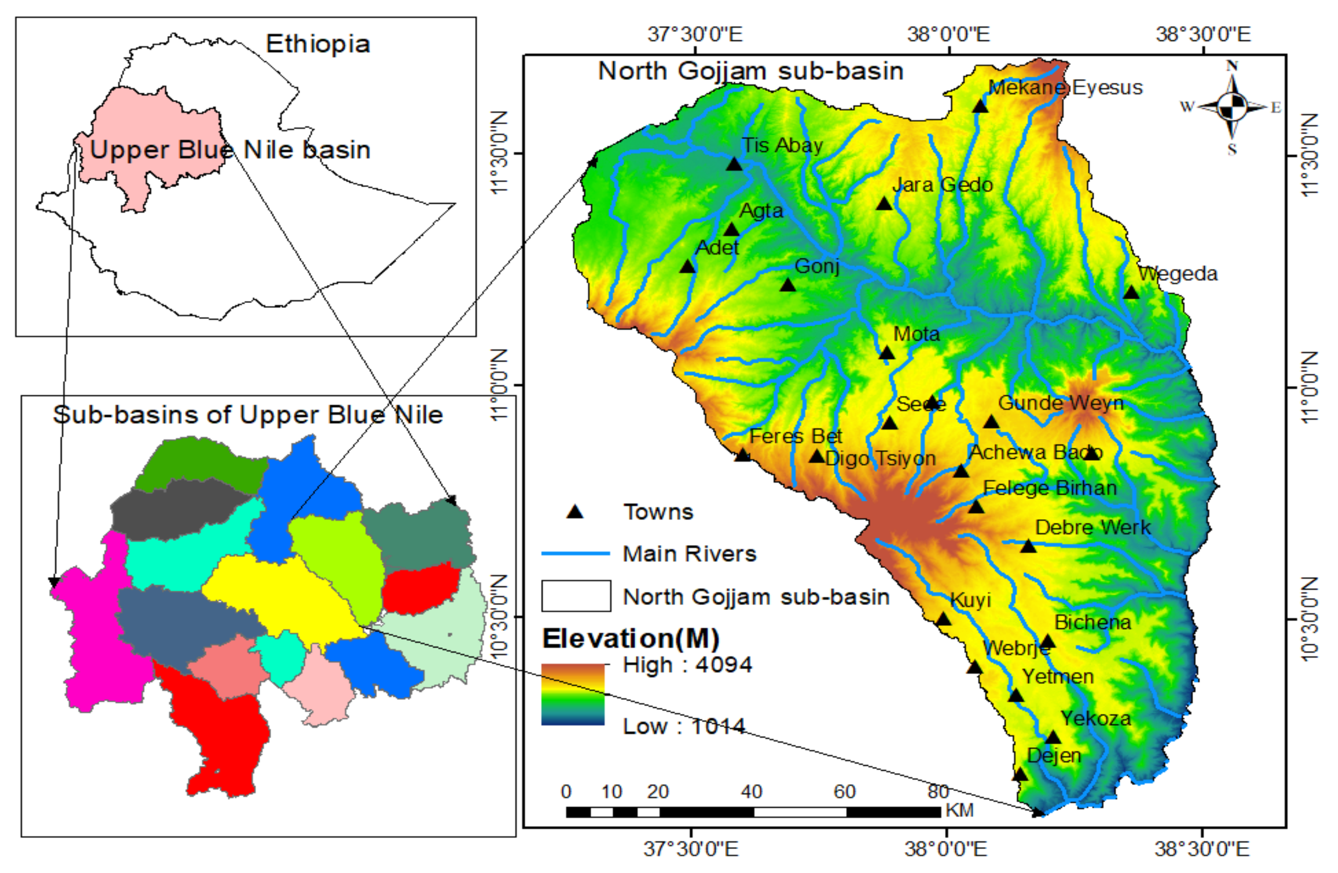
2.1. Description of the Study Area
2.2. Data Sources
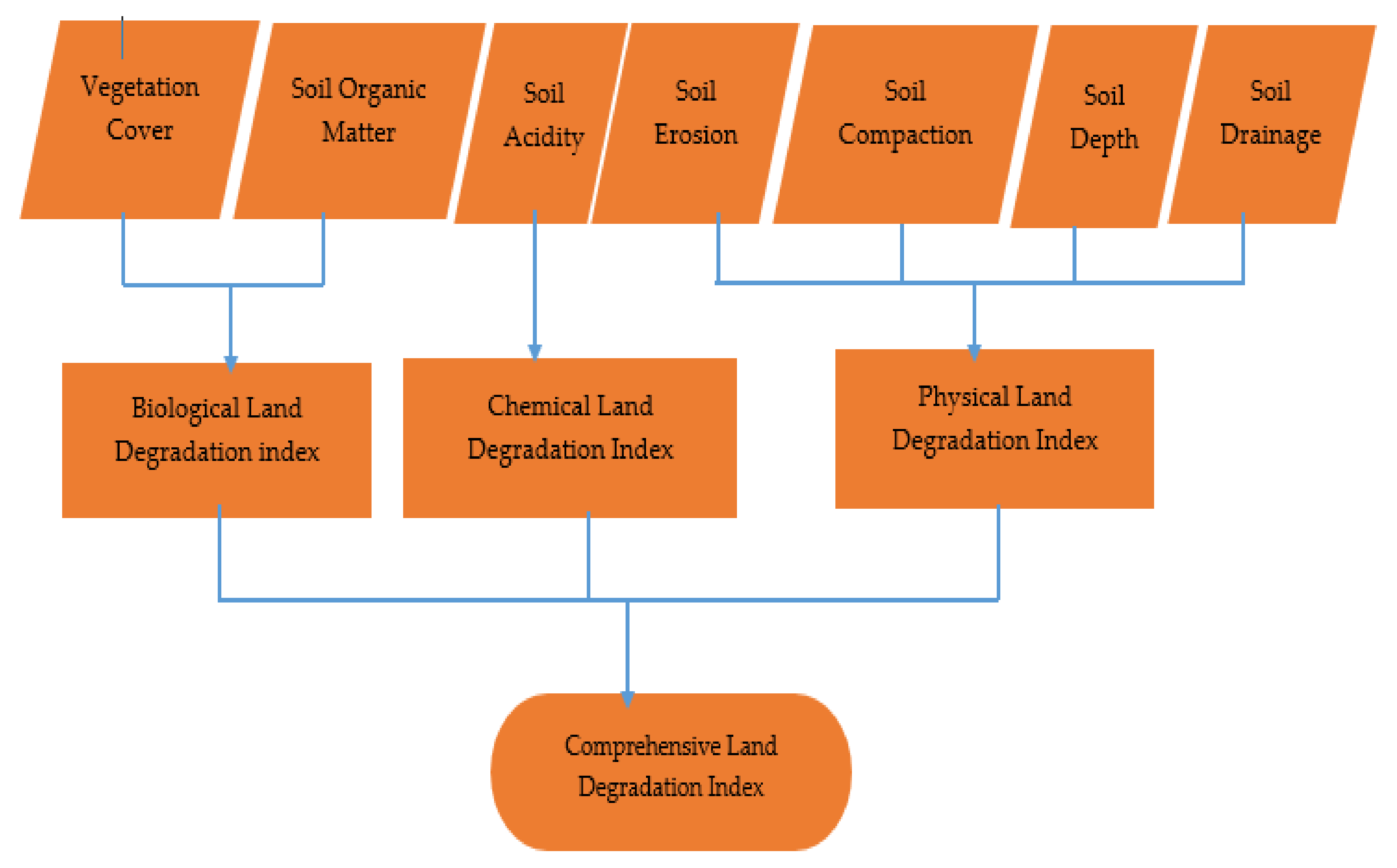
2.3. Spatial Multi-Criteria Analysis (MCA)
2.3.1. Develop Physical Land Degradation Indicators
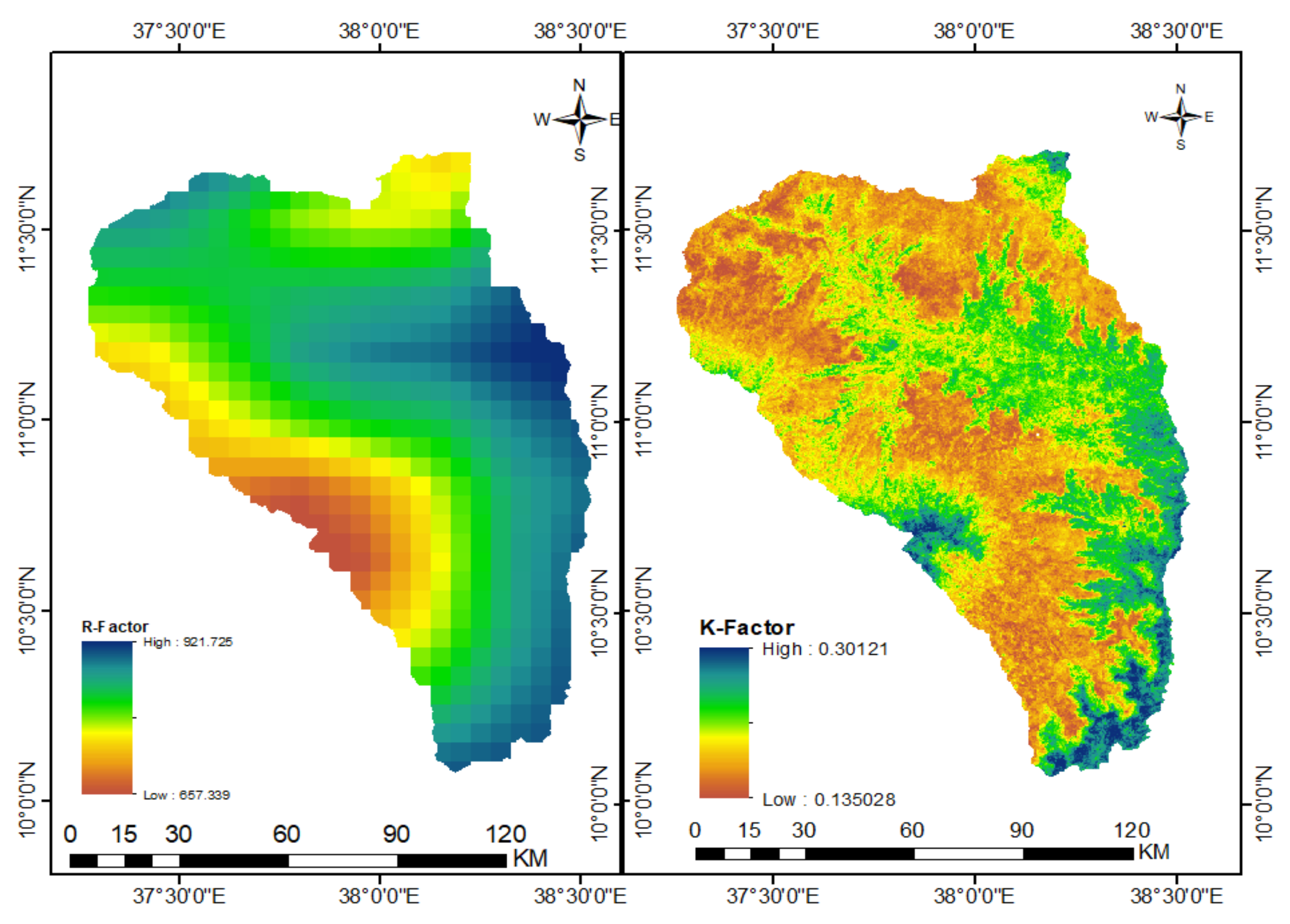
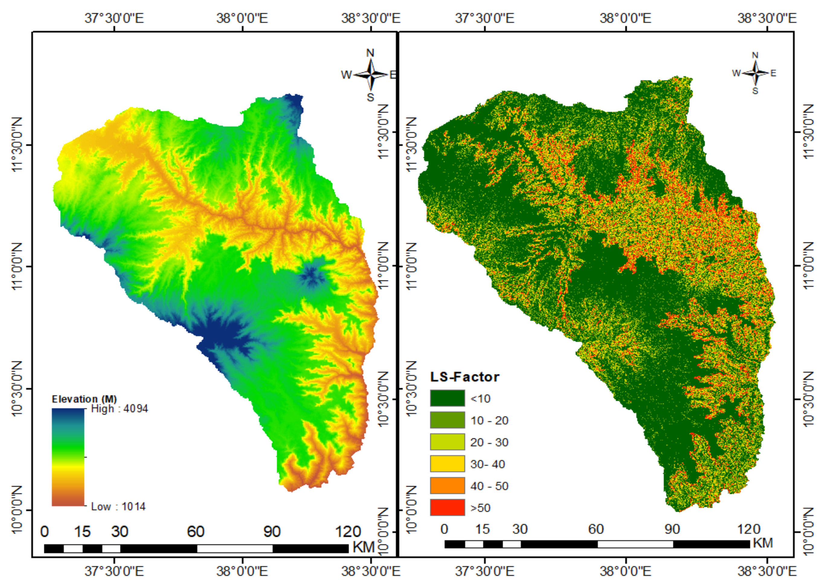
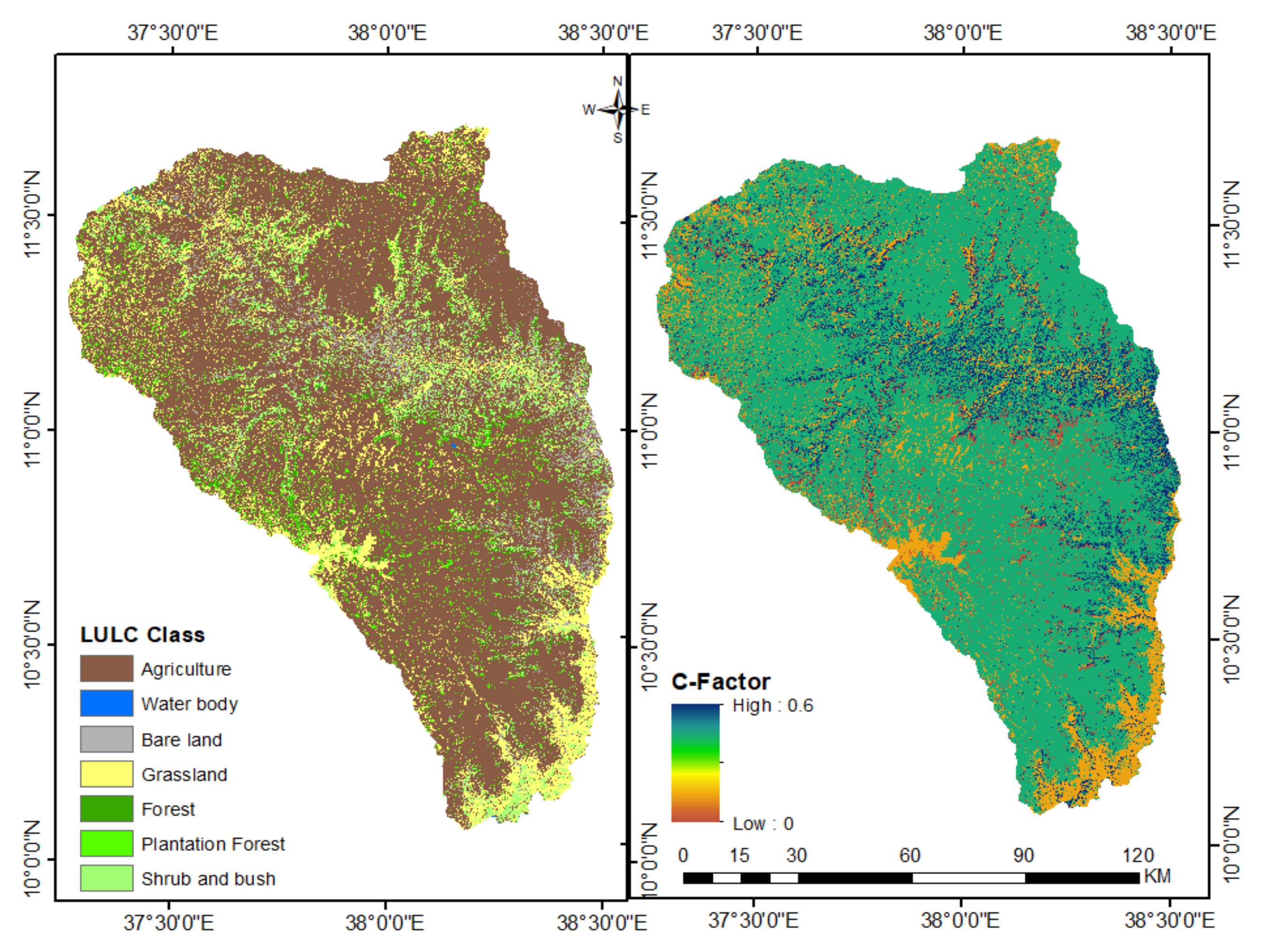
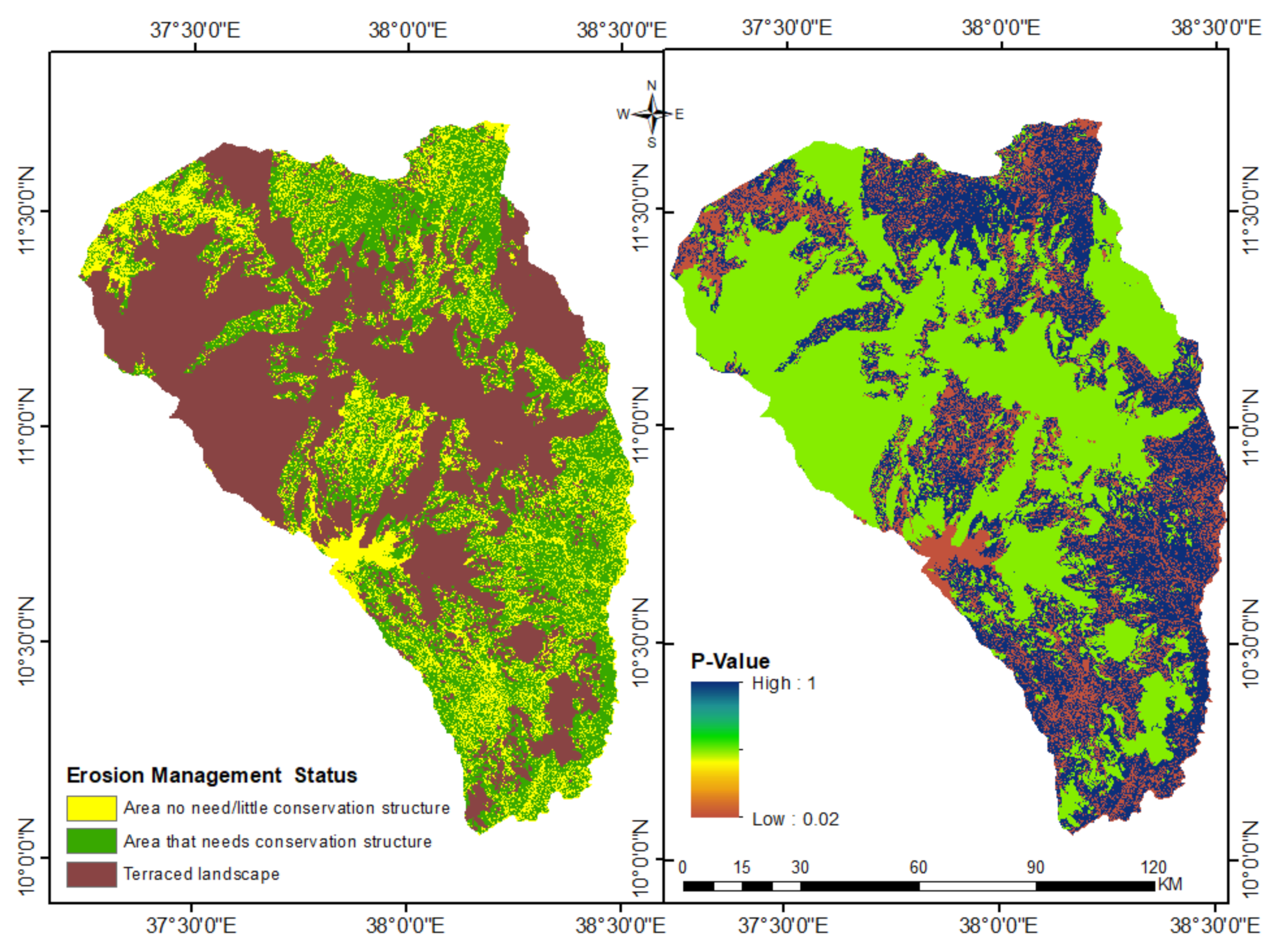
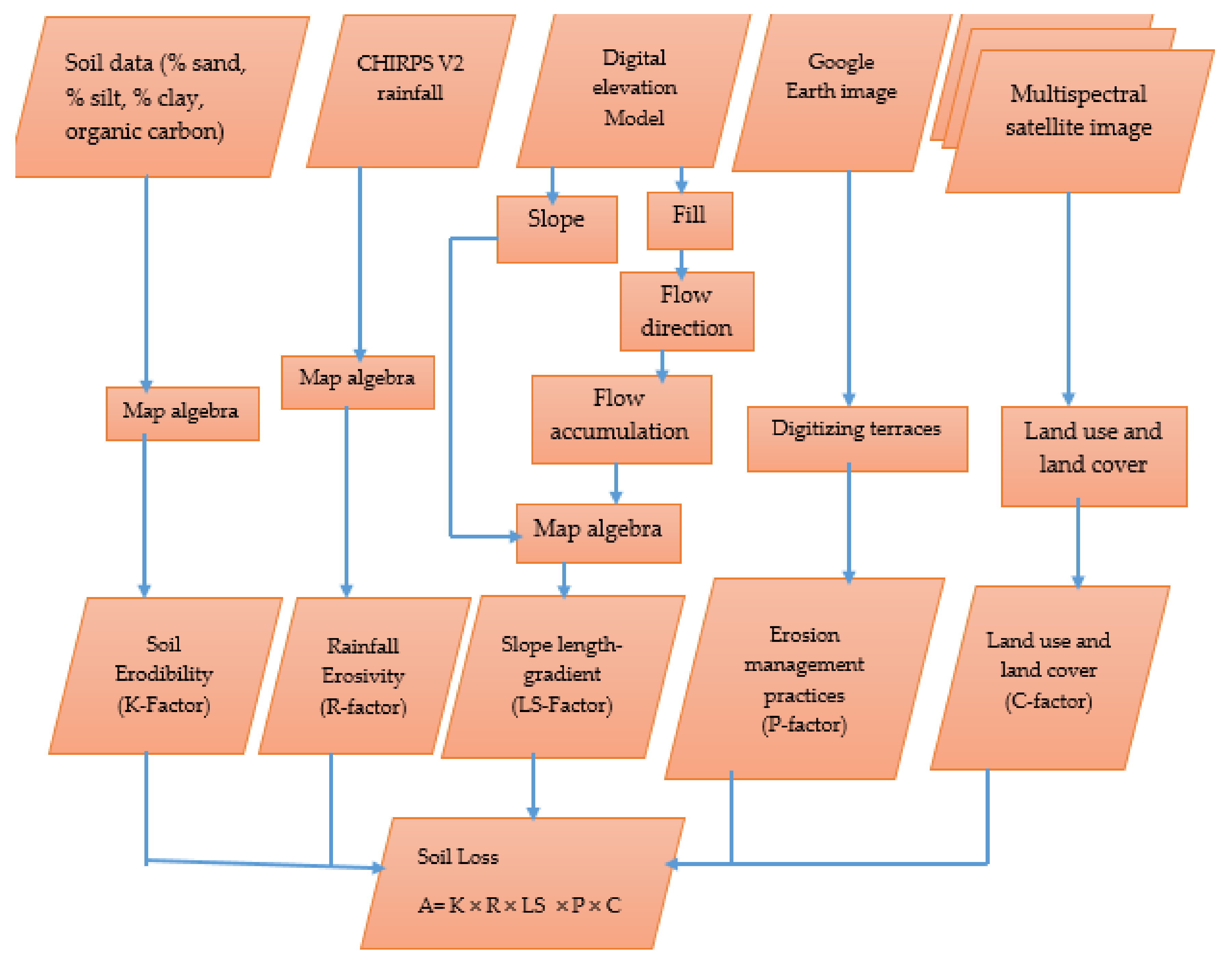
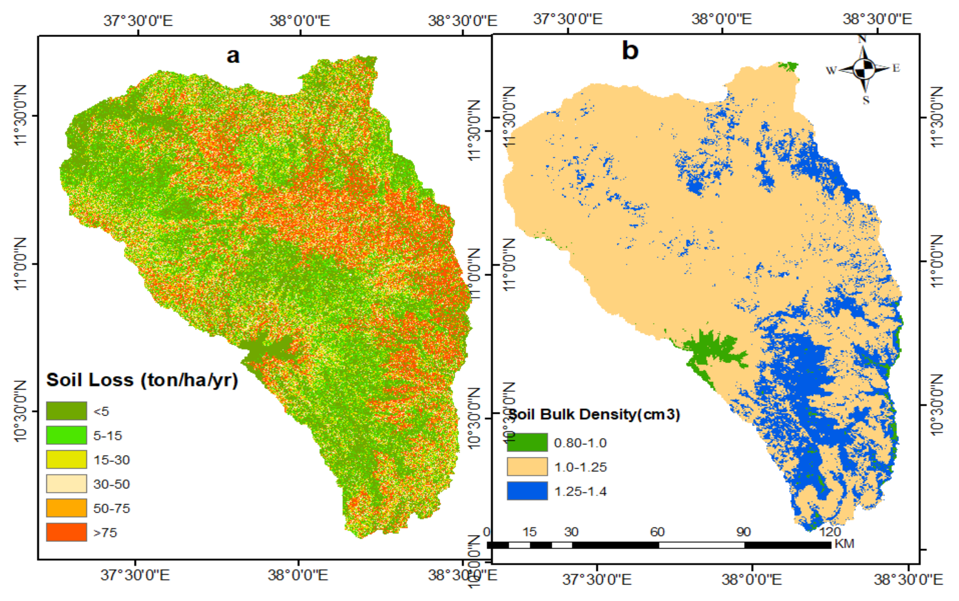
Soil Loss Estimation Using RUSLE Model
Soil Compaction
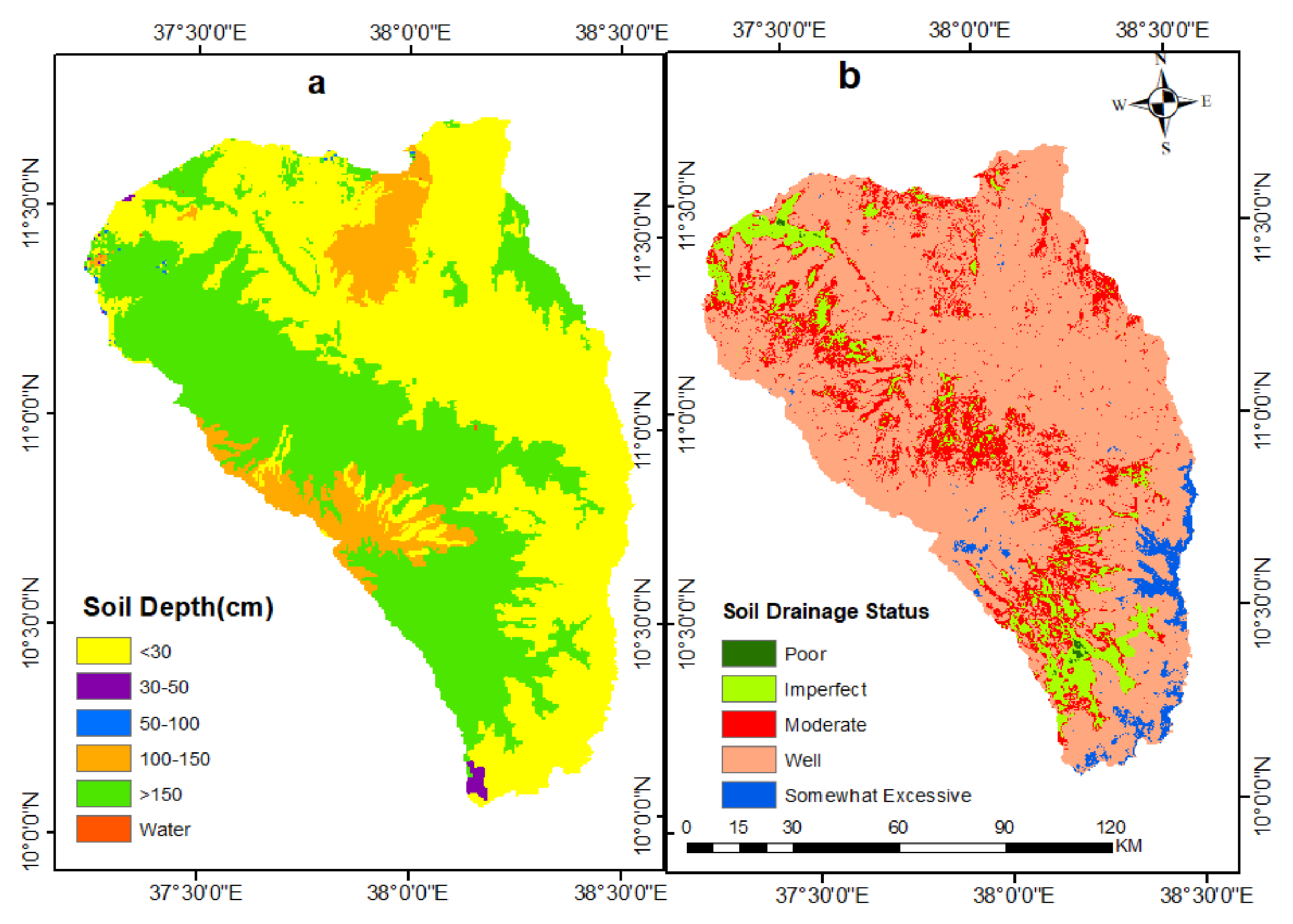
Soil Drainage
Soil Depth
2.3.2. Develop Biological Land Degradation Indicators
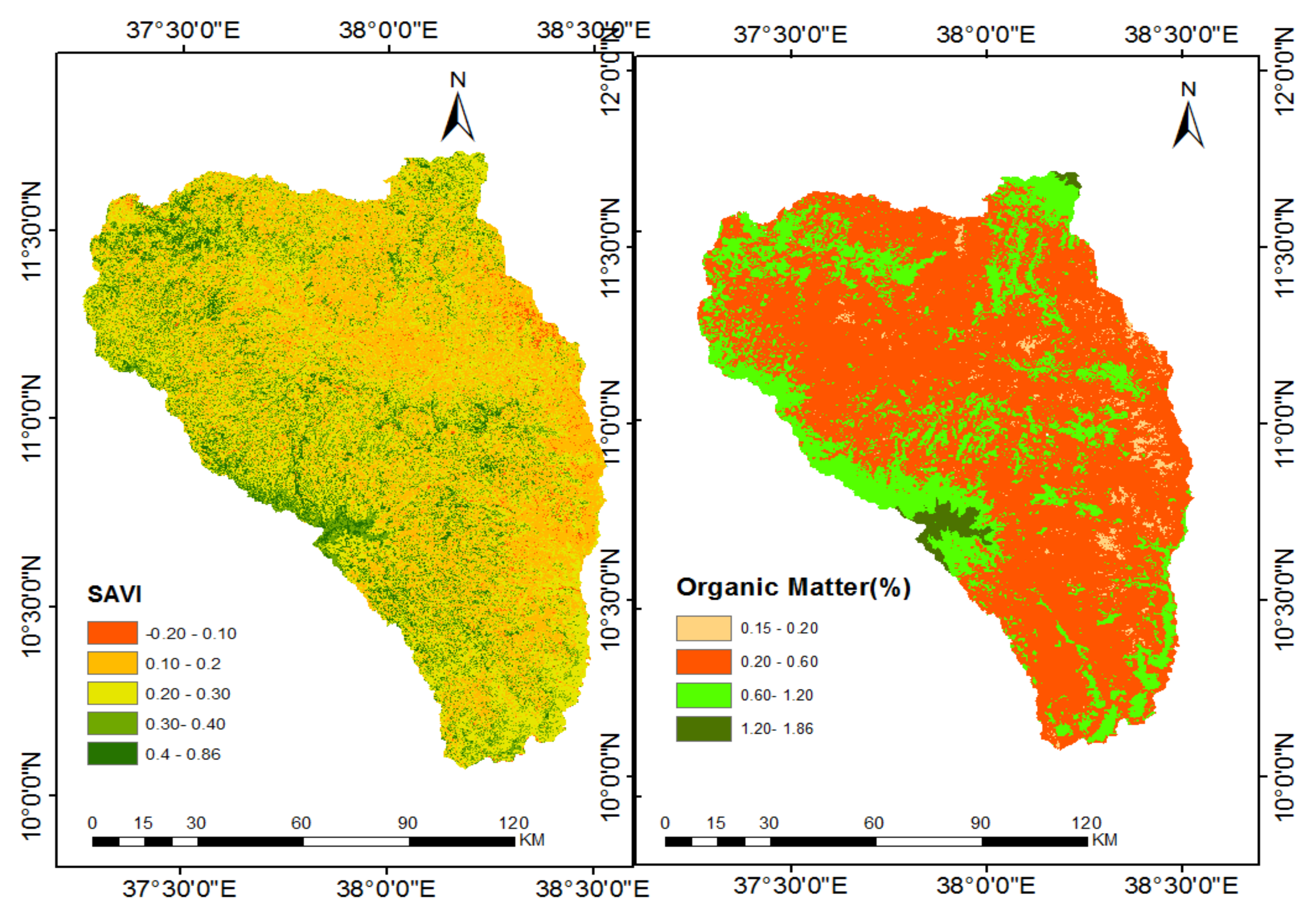
Vegetation Cover
Soil Organic Matter (SOM)
2.4. Chemical Land Degradation Indicators
3. Results and Discussion
3.1. Physical Land Degradation Indicators
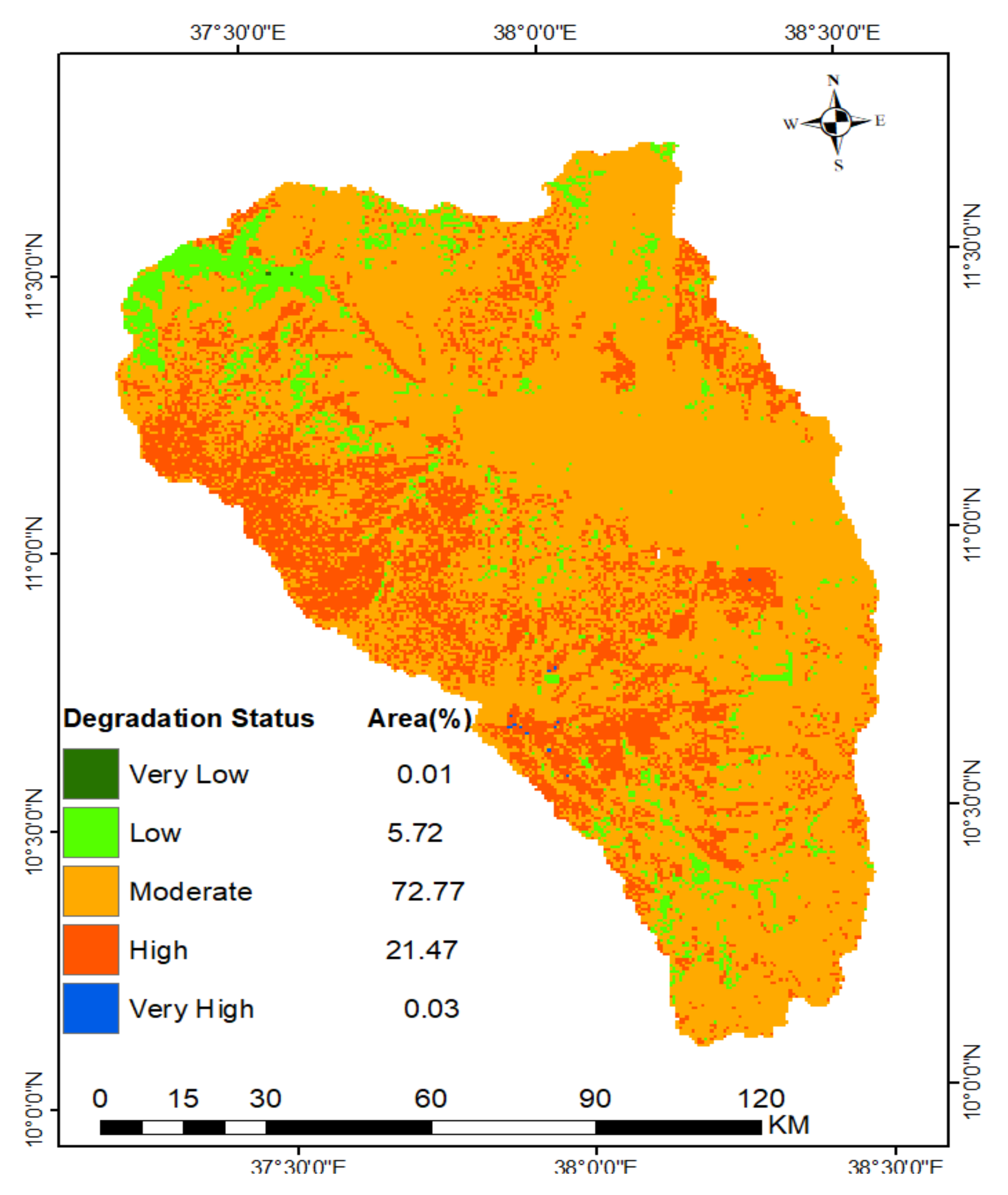
3.2. The State of Physical Land Degradation
3.3. Biological Land Degradation Indicators
3.4. The Status of Biological Land Degradation
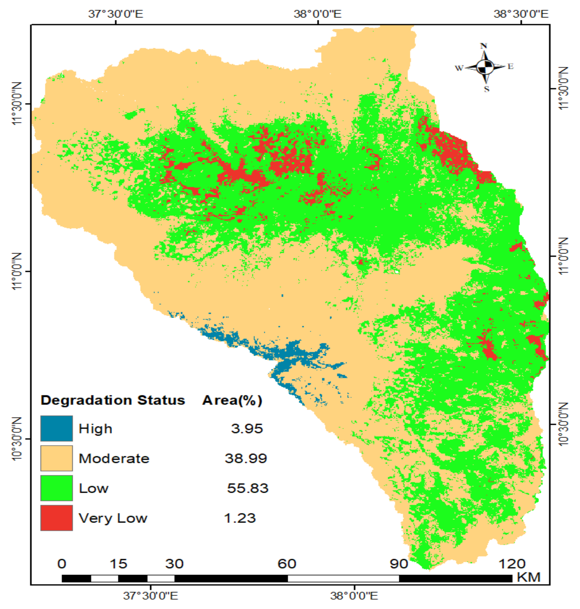
3.5. The State of Chemical Land Degradation
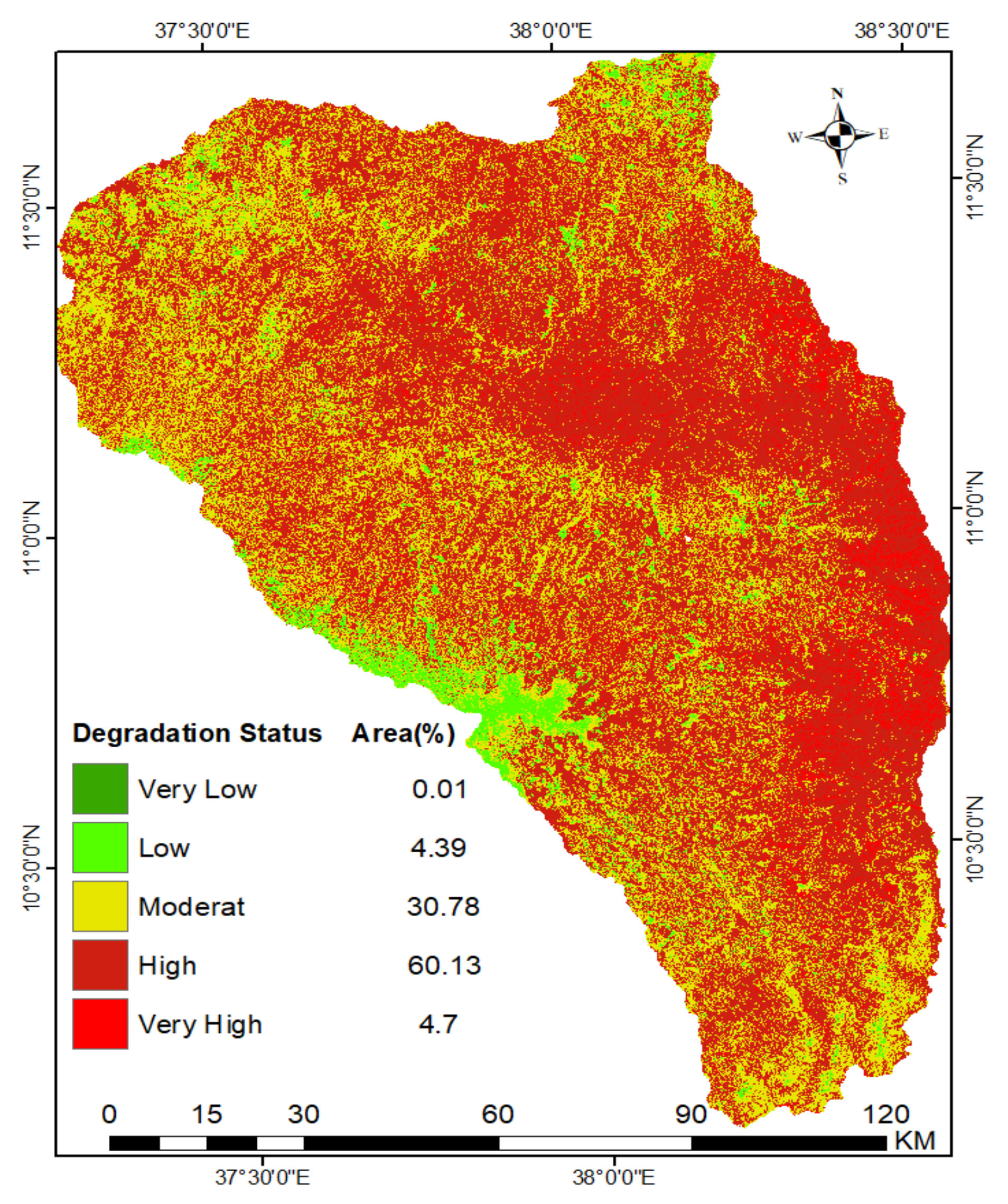
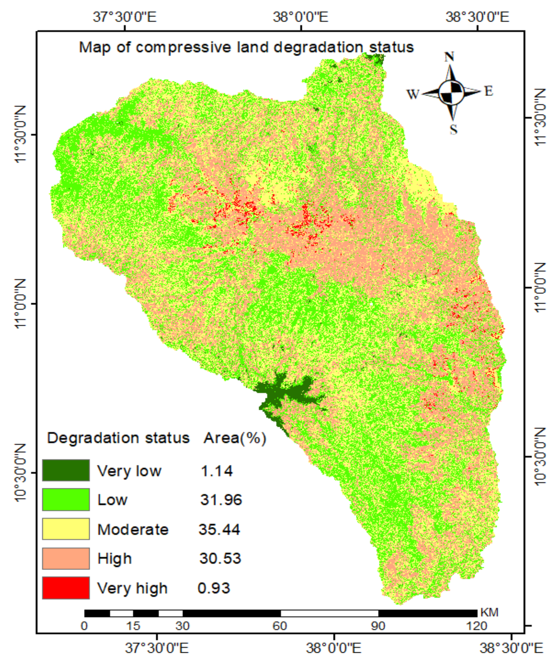
3.6. The Status of Comprehensive Land Degradation in the North Gojjam Sub-Basin
4. Conclusions and Policy Implications
Author Contributions
Funding
Institutional Review Board Statement
Informed Consent Statement
Conflicts of Interest
References and Note
- Nkonya, E.; von Braun, J.; Mirzabaev, A.; Le, Q.B.; Kwon, H.Y.; Kirui, O. Economics of Land Degradation Initiative: Methods and Approach for Global and National Assessments; ZEF—Discussion Papers on Development Policy No. 183; Center for Development Research: Bonn, Germany, 2013; p. 41. [Google Scholar]
- Sadik-Zada, E.R. Distributional Bargaining and the Speed of Structural Change in the Petroleum Exporting Labor Surplus Economies. Eur. J. Dev. Res. 2020, 32. [Google Scholar] [CrossRef]
- Sadik-zada, E.R. Natural resources, technological progress, and economic modernization. Rev. Dev. Econ. 2020, 7, 1–24. [Google Scholar] [CrossRef]
- Le, Q.B.; Nkonya, E.; Mirzabaev, A. Biomass Productivity-Based Mapping of Global Land Degradation Hotspots. In Economics of Land Degradation and Improvement—A Global Assessment for Sustainable Development; Nkonya, E., Mirzabaev, A., von Braun, J., Eds.; Springer: Cham, Switzerland, 2016. [Google Scholar] [CrossRef]
- El-gammal, M.I.; Ali, R.R.; Samra, R.M.A. Science Direct GIS-based land degradation risk assessment of Damietta governorate, Egypt. Egypt J. Basic Appl. Sci 2015, 2, 183–189. [Google Scholar] [CrossRef][Green Version]
- Economy of Land Degradation (ELD) Initiative. The Rewards of Investing in Sustainable Land Management. Interim Report for the Economics of Land Degradation Initiative: A Global Strategy for Sustainable Land Management. 2013. Available online: www.eld-initiative.org (accessed on 18 November 2018).
- UNCCD. Climate change and land degradation: Bridging knowledge and stakeholders Outcomes. In Proceedings of the UNCCD 3rd Scientific Conference, Cancun, Mexico, 9–12 March 2015. [Google Scholar]
- Nellemann, C. The Environmental Food Crisis: The Environment’s Role in Averting Future Food Crises: A UNEP Rapid Response Assessment. UNEP/Earth Print. 2009. Available online: https://www.grida.no/publications/154 (accessed on 18 November 2018).
- Obalum, S.E.; Buri, M.M.; Nwite, J.C.; Watanabe, Y.; Igwe, C.A.; Wakatsuki, T. Soil Degradation-Induced Decline in Productivity of Sub-Saharan African Soils: The Prospects of Looking Downwards the Lowlands with the Sawah Ecotechnology. Appl. Environ. Soil Sci. 2012, 2012. [Google Scholar] [CrossRef]
- United Nations Convention to Combat Desertification (UNCCD). Refinement of the Set of Impact Indicators on Strategic Objectives 1, 2 and 3 Recommendations of the ad hoc Advisory Group of Technical Experts. ICCD/COP (11) /CST/2. Available online: https://www.unccd.int/sites/default/files/sessions/documents/ICCD_COP11_CST_2/cst2eng.pdf (accessed on 27 November 2018).
- Berry, L.; Olson, J.; Campbell, D. (Eds.) Assessing the Extent, Cost and Impact of Land Degradation at the National Level: Findings and Lessons Learned from Seven Pilot Case Studies; Commissioned by Global Mechanism with Support from World Bank; World Bank: Washington, DC, USA, 2003. [Google Scholar]
- Hurni, H.; Bantider, A.; Debele, B.; Ludi, E. Land degradation and sustainable land management in the Highlands of Ethiopia. Glob. Chang. Sustain. Dev. 2010. [Google Scholar] [CrossRef]
- Zeleke, A.G.; Hurni, H. Implications of Land Use and Land Cover Dynamics for Mountain Resource Degradation in the Northwestern Ethiopian Highlands. Mt. Res. Dev. 2001, 21, 184–191. [Google Scholar] [CrossRef]
- Gebreselassie, S.; Kiuri, O.K.; Mirzabaev, A. Economics of Land Degradation and Improvement in Ethiopia-Aglobal Assessement for Sustenable Development. In Economics of Land Degradation and Improvement—A Global Assessment for Sustainable Development; Nkonya, E., Mirzabaev, A., von Braun, J., Eds.; Springer: Cham, Switzerland, 2016. [Google Scholar] [CrossRef]
- FAO. Ethiopian Highlands Reclamation Study; Final Report; FAO: Rome, Italy, 1986. [Google Scholar]
- Oo, O.; Sl, G.; Do, G. Analyzing the Rate of Land Use and Land Cover Change and Determining the Causes of Forest Cover Change in Gog District, Gambella Regional. J. Remote Sens. GIS 2017, 6. [Google Scholar] [CrossRef]
- Reusing, M.; Schneider, T.; Ammer, U. Modelling soil loss rates in the Ethiopian Highlands by integration of high resolution MOMS-02/D2- stereo-data in a GIS. Int. J. Remote Sens. 2010, 21, 1885–1896. [Google Scholar] [CrossRef]
- Gebru, T.D. Deforestation in Ethiopia: Causes, Impacts and Remedy. Int. J. Energy Dev. Res. 2016, 4, 204–209. [Google Scholar]
- Gashaw, T.; Bantider, A.; Mahari, A. Evaluations of Land Use/Land Cover Changes and Land Degradation in Dera District, Full Length Research Paper: GIS and Remote Sensing Based Analysis. Int. J. Sci. Res. Environ. Sci. 2014. [Google Scholar] [CrossRef]
- Haregeweyn, N.; Tsunekawa, A.; Nyssen, J.; Poesen, J.; Tsubo, M.; Tsegaye Meshesha, D.; Schütt, B.; Adgo, E.; Tegegne, F. Soil erosion and conservation in Ethiopia: A review. Prog Phys. Geogr. 2015, 39, 750–774. [Google Scholar] [CrossRef]
- Molla, T.; Sisheber, B. Estimating soil erosion risk and evaluating erosion control measures for soil conservation planning at Koga watershed in the highlands of Ethiopia. Solid Earth 2017, 8, 13–25. [Google Scholar] [CrossRef]
- Meseret, D.; Gangadhara, M.H. Integration of Geospatial Technologies with RUSLE for Analysis of Land Use/Cover Change Impact on Soil erosion: Case study in Rib watershed, north—western highland Ethiopia. Environ. Earth Sci. 2017, 76, 1–14. [Google Scholar] [CrossRef]
- Esa, E.; Assen, M.; Legass, A. Implications of land use/cover dynamics on soil erosion potential of agricultural watershed, northwestern highlands of Ethiopia. Environ. Syst Res. 2018. [Google Scholar] [CrossRef]
- Tamene, L.; Adimassu, Z.; Aynekulu, E.; Yaekob, T. International Soil and Water Conservation Research Estimating landscape susceptibility to soil erosion using a GIS-based approach in Northern Ethiopia. Int. Soil Water Conserv. Res. 2017, 5, 221–230. [Google Scholar] [CrossRef]
- Olika, G.; Iticha, B. Assessment of Soil Erosion Using RUSLE and GIS Techniques: A Case of Fincha’a Watershed, Western Ethiopia. Am.-Euras. J. Agric. Environ. Sci. 2019, 19, 31–36. [Google Scholar] [CrossRef]
- Haregeweyn, N.; Tsunekawa, A.; Poesen, J.; Tsubo, M.; Meshesha, D.T.; Fenta, A.A.; Nyssen, J.; Adgo, E. Comprehensive assessment of soil erosion risk for better land use planning in river basins: Case study of the Upper Blue Nile River. Sci. Total Environ. 2017, 574, 95–108. [Google Scholar] [CrossRef]
- Agegnehu, G.; Yirga, C. Soil Acidity Management; Ethiopian Institute of Agriculture Research: Addis Ababa, Ethiopia, 2019; ISBN 9789994466597. [Google Scholar]
- Simane, B.; Zaitchik, B.F.; Foltz, J.D. Agroecosystem specific climate vulnerability analysis: Application of the livelihood vulnerability index to a tropical highland region. Mitig. Adapt. Strateg. Glob. Chang. 2016, 21, 39–65. [Google Scholar] [CrossRef]
- Ewunetu, A.; Simane, B.; Teferi, E.; Zaitchik, B.F. Land Cover Change in the Blue Nile River Headwaters: Farmers’ Perceptions, Pressures, and Satellite-Based Mapping. Land 2021, 10, 68. [Google Scholar] [CrossRef]
- Bewket, W.; Teferi, E. Assessment of soil erosion hazard and prioritization for treatment at the watershed level: Case study in the Chemoga watershed, Blue Nile basin, Ethiopia. Land Degrad. Dev. 2009, 20, 609–622. [Google Scholar] [CrossRef]
- Moore, I.D.; Wilson, J.P. Length-slope factors for the Revised Universal Soil Loss Equation: Simplified method of estimation. J. Soil Water Conserv. 1992, 47, 423–428. [Google Scholar]
- Lu, D.; Batistella, M.; Moran, P.M.E. Mapping and monitoring land degradation risks in the western brazilian amazon using multitemporal landsat TM/ETM+ images. Land Degrad Dev. 2006, 18, 609–622. [Google Scholar] [CrossRef]
- Rahman, R.; Shi, Z.H.; Chongfa, C. Soil erosion hazard evaluation—An integrated use of remote sensing, GIS and statistical approaches with biophysical parameters towards management strategies. Ecol. Model. 2009, 220, 1724–1734. [Google Scholar] [CrossRef]
- Chabrillat, S. Land degradation indicators: Spectral indices. Ann. Arid Zone 2006, 45, 331. [Google Scholar]
- FAO. Methodological Framework for Land Degradation Assessment in Dry Lands (LADA) (Simplified Version): Report on a Consultancy as Visiting Scientist by Rural Ponce- Hernandez with Parviz Koohafkan; FAO-UN, Land and Water Development Division: Rome, Italy, 2004. [Google Scholar]
- Abdelrahman, M.A.E.; Natarajan, A.; Hegde, R.; Prakash, S.S. Assessment of land degradation using comprehensive geostatistical approach and remote sensing data in GIS-model builder. Egypt J. Remote Sens. Space Sci. 2018. [Google Scholar] [CrossRef]
- Rabia, A.H. GIS spatial modeling for land degradation assessment in Tigray, Ethiopia. In Proceedings of the 8th International Soil Science Congress on Land Degradation and Challenges in Sustainable Soil Management, Çeşme-Izmir, Turkey, 15–17 May 2012; pp. 161–167. [Google Scholar]
- Oldeman, L.; van Lynden, G. Revisiting the Glasod Methodology; Working Paper and Preprint, 96/03; International Soil Reference and Information Centre: Wageningen, The Netherlands, 1996. [Google Scholar]
- Agyemang, I. Assessing the driving forces of environmental degradation in Northern Ghana: Community truthing approach. Afr. J. Hist. Cult. 2012, 4, 59–68. [Google Scholar] [CrossRef]
- CSA. Agricultural Sample Survey 2015/2016; Report on Livestock and Livestock Characteristics (Private Peasant Holdings); Central Statistical Agency: Addis Ababa, Ethiopia, 2016; Volume II. [Google Scholar]
- Simane, B.; Zaitchik, B.F.; Ozdogan, M. Agroecosystem Analysis of the Choke Mountain. Sustainability 2013, 5, 592–616. [Google Scholar] [CrossRef]
- Ethiopian National Metrological Agency. Available online: http://www.ethiomet.gov.et/ (accessed on 12 January 2018).
- Yilma, A.D.; Awulachew, S.B. Characterization and Atlas of the Blue Nile Basin and Its Sub Basin; IWMI: Anand, India, 2009. [Google Scholar]
- USGS. Earth Explorer. Available online: http://glovis.usgs.gov (accessed on 12 January 2018).
- ASTER_GDEM. Advanced Spectrum Thermal Emission and Reflectance Radiometer-Global Digital Elevation Map Version 3. Available online: http://gdex.cr.usgs.gov/gdex/ (accessed on 12 January 2018).
- Abdelmoneim, H.; Reda, M.; Moghazy, H.M. Evaluation of TRMM 3B42V7 and CHIRPS Satellite Precipitation Products as an Input for Hydrological Model over Eastern Nile Basin. Earth Syst. Environ. 2020. [Google Scholar] [CrossRef]
- USAID. CHIRPS: Rainfall Estimasion from Rainfall and Sattelite Obervation, the Regent of the University of California, UC Senta Barbara, Senta Barbara, CA93106. Available online: https://www.che.ucsb.edu/data/chirps/ (accessed on 21 November 2019).
- Hengl, T.; De Jesus, J.M.; Heuvelink, G.B.M.; Ruiperez Gonzalez, M.; Kilibarda, M.; Blagotić, A.; Shangguan, W.; Wright, M.N.; Geng, X.; Bauer-Marschallinger, B.; et al. SoilGrids250m: Global Gridded Soil Information Based on Machine Learning. PLoS ONE 2017, 12, e0169748. [Google Scholar] [CrossRef] [PubMed]
- Google. Land Use Map; Google Earth Pro. USGS: Reston, VA, USA, 2018. [Google Scholar]
- Jaiswal, R.K.; Ghosh, N.C.; Galkate, R.V.; Thomas, T. Multi Criteria Decision Analysis (MCDA) for watershed. Aquat. Procedia 2015, 4, 1553–1560. [Google Scholar] [CrossRef]
- Ananda, J.; Herath, G. A critical review of multi-criteria decision making methods with special reference to forest management and planning. Ecol. Econ. 2009, 68, 2535–2548. [Google Scholar] [CrossRef]
- Jafari, S.; Zaredar, N. Land Suitability Analysis using Multi Attribute Decision Making Approach. Int. J. Environ. Sci. Dev. 2010, 1, 441–445. [Google Scholar] [CrossRef]
- Belal, A.B.; Sciences, S.; Abu-hashim, M. Land Evaluation Based on GIS-Spatial Multi-Criteria Evaluation (SMCE) for Agricultural Development in Dry Wadi, Eastern Desert. Int. J. Soc. Sci. 2015, 10, 100–116. [Google Scholar] [CrossRef]
- Hajkowicz, S. A comparison of multiple criteria analysis and unaided approaches to environmental decision making. Environ. Sci. Policy 2007, 10, 177–184. [Google Scholar] [CrossRef]
- Zolekar, R.B.; Bhagat, V.S. Multi-criteria land suitability analysis for agriculture in hilly zone: Remote sensing and GIS approach. Comput. Electron. Agric. 2015, 118, 300–321. [Google Scholar] [CrossRef]
- Sałabun, W.; Ziemba, P.; Wątróbski, J. The rank reversals paradox in management decisions: The comparison of the AHP and COMET methods. Smart Innov. Syst. Technol. 2016, 56, 181–191. [Google Scholar] [CrossRef]
- Şener, Ş.; Şener, E.; Nas, B.; Karagüzel, R. Combining AHP with GIS for landfill site selection: A case study in the Lake Beyşehir catchment area (Konya, Turkey). Waste Manag. 2010, 30, 2037–2046. [Google Scholar] [CrossRef] [PubMed]
- Saaty, T.; Vargas, L. Methods, Concepts and Applications of the Analytic Hierarchy Process; Kluwer Academic Publishers: Boston, MA, USA, 2001. [Google Scholar]
- Khoshabi, P.; Nejati, E.; Ahmadi, S.F.; Chegini, A.; Makui, A.; Ghousi, R. Developing a multi-criteria decision making approach to compare types of classroom furniture considering mismatches for anthropometric measures of university students. PLoS ONE 2020, 15, e0239297. [Google Scholar] [CrossRef] [PubMed]
- Saaty, T.L. The Analytic Hierarchy Process; McGraw-Hill: New York, NY, USA, 1980. [Google Scholar]
- Ashtiani, B.; Haghighirad, F.; Makui, A.; Montazer, G. Extension of fuzzy TOPSIS method based on interval-valued fuzzy sets. Appl. Soft Comput. 2009, 9, 457–461. [Google Scholar] [CrossRef]
- Hajkowicz, S.; Higgins, A. A comparison of multiple criteria analysis techniques for water resource management. Eur. J. Oper. Res. 2008, 184, 255–265. [Google Scholar] [CrossRef]
- Mihajlo Vic, J.; Rajković, P.; Petrović, G.C. ’ irićD. The Selection of the Logistics Distribution Center Location Based on MCDM Methodology in Southern and Eastern Region in Serbia. Oper. Res. Eng. Sci. Theory Appl. 2019, 2, 72–85. [Google Scholar]
- Bhushan, N.; Rai, K. Strategic Decision Making: Applying the Analytic Hierarchy Process, 4th ed.; Springer: New York, NY, USA, 2004; p. 172. [Google Scholar]
- Mokhtarian, M.N.; Sadi-nezhad, S.; Makui, A. A new flexible and reliable interval valued fuzzy VIKOR method based on uncertainty risk reduction in decision making process: An application for determining a suitable location for digging some pits for municipal wet waste landfill. Comput. Ind. Eng. 2014, 78, 213–233. [Google Scholar] [CrossRef]
- Sarin, R.K. Multi-attribute Utility Theory. In Encyclopedia of Operations Research and Management Science; Gass, S.I., Fu, M.C., Eds.; Springer: Boston, MA, USA, 2013; pp. 1004–1006. [Google Scholar]
- Oldeman, L. The Global Extent of Soil Degradation. In ISRIC Bi-Annual Report 1991–1992; International Soil Reference and Information Centre: Wageningen, The Netherlands, 1994; pp. 19–36. [Google Scholar]
- Nachtergaele, F.; Velthuizen, H.; Van Verelst, L.; Batjes, N.H.; Dijkshoorn, J.A.; Engelen, V.W.P.; van Fischer, G.; Montanarella, L.; Petri, M.; Prieler, S. Harmonized World Soil Database. Version 1.0. 2009. Available online: http://www.fao.org/nr/water/docs/Harm-World-Soil-DBv7cv.pdf (accessed on 3 March 2018).
- Nachtergaele, F.O.; Petri, M.; Biancalani, R.; Van Lynden, G.W.; Van Lynden, G.; van Velthuizen, H.; Bloise, M. Global Land Degradation Information System (GLADIS): An Information Database for Land Degradation Assessment at Global Level; LADA Technical Report; 2011; Available online: http://www.fao.org/nr/lada/index.php?option=com_docman&task=doc_download&gid=773&lang=en (accessed on 21 January 2018).
- ASTM. American Society for Testing Materials, Soil Bulk Density Classes. Available online: https://www.sciencedirect.com/topics/earth-and-planetary-sciences/bulk-density (accessed on 21 October 2018).
- USDA. Bulk Density. Soil Quality Indicators, USDA Natural Resources Conservation Service. 2008. Available online: www.nrcs.gov (accessed on 23 December 2017).
- USDA. Soil Quality Indicators, USDA Natural Resources Conservation Service. Available online: www.nrcs.usda.gov (accessed on 23 December 2017).
- Carver, S.J. Integrating Multi-Criteria Evaluation with Geographical Information Systems. Int. J. Geogr. Inf. Sci. 1991, 5, 321–339. [Google Scholar] [CrossRef]
- Eastman, J.R. Multi-criteria evaluation and GIS. Geogr. Inf. Syst. 2012, 1, 493–502. [Google Scholar]
- Malczewski, J. GIS—Based Multicriteria Decision Analysis: A Survey of the Literature. Int. J. Geogr. Inf. Sci. 2006, 20, 703–726. [Google Scholar] [CrossRef]
- Prasad, V.S.; Kousalya, P. Role of Consistency in Analytic Hierarchy Process—Consistency Improvement Methods. Indian J. Sci. Technol. 2017, 10, 1–5. [Google Scholar] [CrossRef]
- Esri Inc. ArcGIS10.5. 2017. Available online: http://www.esri.com/en-us/orginal/product/arcGIS-pro (accessed on 12 January 2018).
- Oldeman, L.; Hakkeling, R.; Sombroek, W. World Map of the Status of Human-Induced Soil Degradation: An Explanatory Note, Second Revised Edition. Available online: http://www.isric.org/sites/default/files/datasets/Glasod.zip (accessed on 17 August 2017).
- Wischmeier, W.H.; Smith, D.D. Predicting Rainfall Erosion Losses: A Guide to Conservation Planning; Agriculture Handbook No. 537; Department of Agriculture: Washington, DC, USA, 1978.
- Farhan, Y.; Nawaiseh, S. Spatial assessment of soil erosion risk using RUSLE and GIS techniques. Environ. Earth Sci. 2015. [Google Scholar] [CrossRef]
- Hurni, H. Erosion-productivity-conservation systems in Ethiopia. In Proceedings of the 4th International Conference on Soil Conservation, Maracacy, Venezuela, 3–9 November 1985. [Google Scholar]
- Renard, K.G.; Foster, G.R. Managing Rangeland Soil Resources: The Universal Soil Loss Equation. Rangelands 1985, 7, 118–122. [Google Scholar]
- Laflen, J.M.; Flanagan, D.C. The development of USLE soil erosion prediction and modeling 1# Introduction 2# Empirical soil erosion prediction in the United States. Int. Soil Water Conserv. Res. 2013, 1, 1–11. [Google Scholar] [CrossRef]
- Yang, X.; Gray, J.; Chapman, G.; Zhu, Q.; Tulau, M.; McInnes-Clarke, S. Digital mapping of soil erodibility for water erosion in New South Wales, Australia. Soil Res. 2018, 56, 158–170. [Google Scholar] [CrossRef]
- Romkens, M.M.; Young, R.A.; Poesen, J.A.; McCool, D.K.; El-Swaify, S.A.; Bradford, J.M. Soil erodibility factor (K.). In Predicting Soil Erosion by Water: A Guide to Conservation Planning with the Revised Universal Soil Loss Equation (RUSLE); Renard, K.G., Foster, G.R., Weesies, G.A., McCool, D.K., Yoder, D.C., Eds.; U.S. Government Printing Office: Washington, DC, USA, 1997; pp. 65–100. [Google Scholar]
- Song, X.; Du, L.; Kou, C.; Ma, Y. Assessment of soil erosion in water source area of the Danjiangkou reservoir using USLE and GIS. In Proceedings of the Second 73 International Conference on Information Computing and Applications, Qinhuangdao, China, 28–31 October 2011; Springer: Berlin/Heidelberg, Germany, 2011; pp. 57–64. [Google Scholar]
- Ganasri, B.P.; Ramesh, H. Geoscience Frontiers Assessment of soil erosion by RUSLE model using remote sensing and GIS—A case study of Nethravathi Basin. Geosci. Front. 2016, 7, 953–961. [Google Scholar] [CrossRef]
- Amsalu, T.; Mengaw, A. GIS Based Soil Loss Estimation Using RUSLE Model: The Case of Jabi Tehinan Woreda, Ethiopia. Nat. Resourc. 2014, 5, 616–626. [Google Scholar] [CrossRef]
- Renard, K.G.; Yoder, D.C.; Lightle, D.T.; Dabney, S.M. Universal soil loss equation and revised universal soil loss equation. In Handbook of Erosion Modelling, 1st ed.; Morgan, R.P.C., Nearing, M.A., Eds.; Blackwell Publishing Ltd.: New York, NY, USA, 2011. [Google Scholar]
- ERDAS. ERDAS Imagine 2014; Hexagon Geospatial: Peachtree Corners, GA, USA, 2014. [Google Scholar]
- Gelagay, H.S.; Minale, A.S. Soil loss estimation using GIS and Remote sensing techniques: A case of Koga watershed, Northwestern Ethiopia. Int. Soil Water Conserv. Res. 2016, 4, 126–136. [Google Scholar] [CrossRef]
- Zerihun, M.; Mohammedyasin, M.S.; Sewnet, D.; Adem, A.A.; Lakew, M. Assessment of soil erosion using RUSLE, GIS and remote sensing in NW Ethiopia. Geoderma Reg. 2018. [Google Scholar] [CrossRef]
- Tiruneh, G.; Ayalew, M. Soil loss estimation using geographic information system in enfraz watershed for soil conservation planning in highlands of Ethiopia. Int. J. Agric. Res. Innov. Technol. 2016, 5, 21–30. [Google Scholar] [CrossRef]
- Panagos, P.; Borrelli, P.; Meusburger, K.; Zanden, E.H.; Van Der, P.J.; Alewell, C. ScienceDirect Modelling the effect of support practices (P-factor) on the reduction of soil erosion by water at European scale. Environ. Sci. Policy 2015, 51, 23–34. [Google Scholar] [CrossRef]
- Miheretu, B.A.; Yimer, A.A. Estimating soil loss for sustainable land management planning at the Gelana sub-watershed, northern highlands of Ethiopia. Int. J. River Basin Manag. 2018, 16, 41–50. [Google Scholar] [CrossRef]
- Yesuph, A.Y.; Dagnew, A.B. Soil erosion mapping and severity analysis based on RUSLE model and local perception in the Beshillo Catchment of the Blue Nile Basin. Environ. Syst Res. 2019. [Google Scholar] [CrossRef]
- Nawaz, M.F.; Bourrié, G. Soil compaction impact and modelling. A review. Agron. Sustain. Dev. 2013, 33, 291–309. [Google Scholar] [CrossRef]
- Abdelrahman, M.A.E.; Natarajan, A.; Srinivasamurthy, C.A. Estimating soil fertility status in physically degraded land using GIS and remote sensing techniques in Chamarajanagar district, Karnataka. Egypt J. Remote Sens. Space Sci. 2016, 19, 95–108. [Google Scholar] [CrossRef]
- Huete, A.R. A soil-adjusted vegetation index (SAVI). Remote Sens. Environ. 1988, 25, 295–309. [Google Scholar] [CrossRef]
- Gilabert, M.; González-Piqueras, J.; Garcıa-Haro, F.; Meliá, J. A Generalized soil-adjusted vegetation index. Remote Sens. Environ. 2002, 82, 303–310. [Google Scholar] [CrossRef]
- Qi, J.; Chehbouni, A.; Huete, A.R.; Kerr, Y.H.; Sorooshian, S. A Modified Soil Adjusted Vegetation Index. Remote Sens. Environ. 1994, 48, 119–126. [Google Scholar] [CrossRef]
- Combs, S.M.; Nathan, M.V.; Brown, J.R. (Eds.) Recommended Chemical Soil Test Procedures for the North Central Region; NCR Publication No. 221; Missouri Agricultural Experiment Station, University of Missouri: Columbia, MO, USA, 1998; pp. 53–58. [Google Scholar]
- Osman, K.T. Soil Degradation, Conservation and Remediation; Springer: New York, NY, USA, 2013. [Google Scholar]
- Kouli, M.; Soupios, P. Soil erosion prediction using the Revised Universal Soil Loss Equation (RUSLE) in a GIS framework, Chania, Northwestern Crete, Greece. Environ. Geol. 2009, 53, 483–497. [Google Scholar] [CrossRef]
- Bewket, W.; Sterk, G. Assessment of soil erosion in cultivated fields using a survey methodology for rills in the Chemoga watershed, Ethiopia. Agric. Ecosyst. Environ. 2003, 97, 81–93. [Google Scholar]
- Herweg, K.; Ludi, E. The performance of selected soil and water conservation measures—Case studies from Ethiopia and Eritrea. Catena 1999, 36, 99–114. [Google Scholar] [CrossRef]
- Belayneh, M.; Yirgu, T.; Tsegaye, D. Runoff and soil loss responses of cultivated land managed with graded soil bunds of different ages in the Upper Blue Nile basin. Ecol. Process. 2020. [Google Scholar] [CrossRef]
- Hurni, H. Land degradation, famine, and land resource scenarios in Ethiopia. In World Soil Erosion and Conservation; Pimentel, D., Ed.; Cambridge University Press: Cambridge, UK, 1993; pp. 27–62. [Google Scholar]
- Gashaw, T.; Tulu, T.; Argaw, M. Erosion risk assessment for prioritization of conservation measures in Geleda watershed, Blue Nile basin, Ethiopia. Environ. Syst. Res. 2017. [Google Scholar] [CrossRef]
- Zeleke, G. Landscape Dynamics and Soil Erosion Process Modeling in the North-Western Ethiopian Highlands; University of Bern: Bern, Switzerland, 2000. [Google Scholar]
- Selassie, Y.G.; Belay, Y. Costs of Nutrient Losses in Priceless Soils Eroded from the Highlands of Northwestern Ethiopia. J. Agric. Sci. 2013, 5, 7. [Google Scholar] [CrossRef]
- Tamene, L.; Le, B.Q. Estimating soil erosion in sub-Saharan Africa based on landscape similarity mapping and using the revised universal soil loss equation (RUSLE). Nutr. Cycl. Agroecosyst. 2015. [Google Scholar] [CrossRef]
- Ethiopian Agricultural Transformation Agency(ATA). Soil Fertility Status and Fertilizer Recommendation Atlas for Amhara Regional State; Ethiopian, ATA: Addis Ababa, Ethiopia, 2017. [Google Scholar]
- Amede, T. Opportunities and Challenges in Reversing Land Degradation: The regional experience. In Natural Resource Degradation and Environmental Concerns in the Amhara National Regional State: Impact on Food Security; Amede, T., Ed.; Ethiopian Soils Science Society: Bahir Dar, Ethiopia, 2003; pp. 173–183. [Google Scholar]
- Abate, E.; Hussein, S.; Laing, M.; Mengistu, F. Soil acidity under multiple land-uses: Assessment of perceived causes and indicators, and nutrient dynamics in small-holders’ mixed-farming system of northwest Ethiopia. Acta Agric. Scand. Sect. B Soil Plant Sci. 2017, 67, 134–147. [Google Scholar] [CrossRef]
- Golla, A.S. Soil Acidity and its Management Options in Ethiopia: A Review. Int. J. Sci. Res. Manag. 2019, 7, 1429–1440. [Google Scholar] [CrossRef]


| LULC | C-Value | Sources |
|---|---|---|
| Natural Forest | 0.01 | [30,93] |
| Plantation Forest | 0.01 | [30,93] |
| Shrub and bush | 0.20 | [30,93] |
| Grassland | 0.05 | [82,93] |
| Agriculture | 0.15 | [82,93] |
| Bare land | 0.60 | [93] |
| Waterbody | 0.00 | [26] |
| Erosion Control Measures | Area in Percent | P-Factor | Sources |
|---|---|---|---|
| Area no need/little conservation structure | 17.79 | 0.02 | [21] |
| Area that need conservation stricture | 33.90 | 1.00 | [21] |
| Terraced landscape | 48.31 | 0.50 | [63] |
| Soil Bulk Density Class | Compaction Status |
|---|---|
| <1 g/cm3 | Low soil compaction |
| 1–1.25 g/cm3 | Medium soil compaction |
| 1.25–1.55 g/cm3 | High soil compaction |
| >1.55 g/cm3 | Very high soil compaction |
| Drainage Class | Level Drainage | Status Description |
|---|---|---|
| 1 | Very poor | Excessively drained |
| 2 | Poor | Somewhat excessively drained |
| 3 | Imperfect | Well drained |
| 4 | Moderate | Moderately well drained |
| 5 | Well | Somewhat poorly drained |
| 6 | Somewhat excessive | Poorly drained |
| 7 | Excessive | Very poorly drained |
| Soil Depth Class | Severity Level | Description |
|---|---|---|
| <30 cm | Very low | Shallow soil |
| 30–50 cm | Low | Moderate shallow soil |
| 50–100 cm | Moderate | Deep shallow soil |
| 100–150 cm | High | Very deep shallow soil |
| >150 cm | Very high | Shallow soil |
| Category in % | Description |
|---|---|
| <0.2 | Very poor soil organic matter content in the soil |
| 0.2–0.6 | Poor soil organic matter content in soil |
| 0.6–1.2 | Medium soil organic matter contentin soil |
| 1.2–2.0 | High soil organic matter contentin the soil |
| >2.0 | Very high soil organic matter contentin the soil |
| pH Value | Description |
|---|---|
| <4.5 | Extremely acid soils include acid sulfate soils |
| 4.5–5.5 | Very acid soils suffering often from toxicity |
| 5.5–7.2 | Acid to neutral soils: these are the best pH conditions for nutrient availability and suitable for most crops |
| 7.2–8.5 | These pH values are indicative of carbonate-rich soils |
| >8.5 | Indicates alkaline soils often very alkaline soils |
| Soil Loss (t/ha/yr.) | Area (ha) | Percentage | Severity Level | Assigned Value | Risk Level |
|---|---|---|---|---|---|
| <5 | 447,872.54 | 31.29 | Very slight | 1 | Very low |
| 5–15 | 276,252.48 | 19.30 | Slight | 2 | Low |
| 15–30 | 193,949.28 | 13.55 | Moderate | 3 | Medium |
| 30–50 | 141,847.78 | 9.91 | High | 4 | High |
| 50–75 | 106,350.05 | 7.43 | Very high | 5 | Very high |
| >75 | 265,087.87 | 18.52 | Sever | 5 | Very high |
| Factor | Classes | Area (Ha) | Percentage | Assigned Value | Degradation Level |
|---|---|---|---|---|---|
| Soil bulk density (g/cm3) | <1 | 19,323.36 | 1.35 | 2 | Low |
| 1–1.25 | 1,158,399.65 | 80.93 | 3 | Moderate | |
| 1.25–1.55 | 253,636.99 | 17.72 | 4 | High | |
| Level of drainage | Poor | 2147.04 | 0.15 | 1 | Very low |
| Imperfect | 110,787.26 | 7.74 | 2 | Low | |
| Moderate | 214,990.27 | 15.02 | 3 | Moderate | |
| Well | 1,064,788.70 | 74.39 | 4 | High | |
| Somewhat excessive | 38,646.72 | 2.70 | 5 | Very high | |
| Soil depth class (cm) | 25–30 | 719,544.67 | 50.27 | 5 | Very high |
| 30–50 | 3864.67 | 0.27 | 4 | High | |
| 50–100 | 1145.09 | 0.08 | 3 | Moderate | |
| 100–150 | 122,524.42 | 8.56 | 2 | Low | |
| >150 | 584,281.15 | 40.82 | 1 | Very low |
| Criteria | Soil Drainage | Soil Depth | Soil Erosion | Soil Compaction | Criteria Weighting |
|---|---|---|---|---|---|
| Soil drainage | 1 | 2 | 3 | 5 | 45 |
| Soil depth | 0.5 | 1 | 2 | 3 | 27 |
| Soil Erosion | 0.33 | 0.50 | 1 | 3 | 20 |
| Soil compaction | 0.2 | 0.33 | 0.33 | 1 | 8 |
| SAVI Classes | Area (ha) | Area (%) | Cover Status | Assigned Values | Degradation Level |
|---|---|---|---|---|---|
| <0.1 | 67,972.77 | 4.75 | Very poor | 5 | Very high |
| 0.1–0.2 | 862,529.67 | 60.26 | Poor | 4 | High |
| 0.2–0.3 | 298,752.48 | 20.87 | Moderate | 3 | Moderate |
| 0.3–0.4 | 172,708.74 | 12.07 | High | 2 | Low |
| >0.4 | 29,396.34 | 2.05 | Very high | 1 | Very low |
| Category in % | Area (Ha) | Percentage (%) | Level of SOM | Severity Level | Assign Value |
|---|---|---|---|---|---|
| 0.15–0.2 | 19,624.79 | 1.73 | Very low | Very high | 5 |
| 0.2–0.6 | 348,429.04 | 72.56 | Low | High | 4 |
| 0.6–1.2 | 1,038,570.57 | 24.34 | Medium | Moderate | 3 |
| 1.2–1.86 | 24,735.61 | 1.37 | High | Low | 2 |
| Criteria | Organic Matter | Vegetation Cover | Criteria Weighting |
|---|---|---|---|
| Organic matter | 1 | 2 | 66.7 |
| Vegetation cover | 0.5 | 1 | 33.3 |
| Soil pH | Area (Ha) | Percentage (%) | Level | Assigned Value |
|---|---|---|---|---|
| 5–5.5 | 56,525.14 | 3.95 | High | 4 |
| 5.5–6.7 | 558,078.76 | 38.99 | Medium | 3 |
| 6.7–7.3 | 799,124.40 | 55.83 | Low | 2 |
| 7.3–7.8 | 17,631.70 | 1.23 | Very low | 1 |
| Criteria | Biophysical Degradation | Physical Degradation | Chemical Degradation | Criteria Weighting |
|---|---|---|---|---|
| Biophysical degradation | 1 | 3 | 7 | 69 |
| Physical degradation | 0.33 | 1 | 2 | 21 |
| Chemical degradation | 0.14 | 0.5 | 1 | 10 |
Publisher’s Note: MDPI stays neutral with regard to jurisdictional claims in published maps and institutional affiliations. |
© 2021 by the authors. Licensee MDPI, Basel, Switzerland. This article is an open access article distributed under the terms and conditions of the Creative Commons Attribution (CC BY) license (http://creativecommons.org/licenses/by/4.0/).
Share and Cite
Ewunetu, A.; Simane, B.; Teferi, E.; Zaitchik, B.F. Mapping and Quantifying Comprehensive Land Degradation Status Using Spatial Multicriteria Evaluation Technique in the Headwaters Area of Upper Blue Nile River. Sustainability 2021, 13, 2244. https://doi.org/10.3390/su13042244
Ewunetu A, Simane B, Teferi E, Zaitchik BF. Mapping and Quantifying Comprehensive Land Degradation Status Using Spatial Multicriteria Evaluation Technique in the Headwaters Area of Upper Blue Nile River. Sustainability. 2021; 13(4):2244. https://doi.org/10.3390/su13042244
Chicago/Turabian StyleEwunetu, Alelgn, Belay Simane, Ermias Teferi, and Benjamin F. Zaitchik. 2021. "Mapping and Quantifying Comprehensive Land Degradation Status Using Spatial Multicriteria Evaluation Technique in the Headwaters Area of Upper Blue Nile River" Sustainability 13, no. 4: 2244. https://doi.org/10.3390/su13042244
APA StyleEwunetu, A., Simane, B., Teferi, E., & Zaitchik, B. F. (2021). Mapping and Quantifying Comprehensive Land Degradation Status Using Spatial Multicriteria Evaluation Technique in the Headwaters Area of Upper Blue Nile River. Sustainability, 13(4), 2244. https://doi.org/10.3390/su13042244