Article

Adding Technology Sustainability Evaluation to Product Development: A Proposed Methodology and an Assessment Model

by
André Souza Oliveira
1,2,
Bruno Caetano dos Santos Silva
1,2,
Cristiano Vasconcellos Ferreira
3,
Renelson Ribeiro Sampaio
2,
Bruna Aparecida Souza Machado
2 and
Rodrigo Santiago Coelho
1,2,*
1
SENAI CIMATEC, SENAI Innovation Institute—Forming and Materials Joining, Av. Orlando Gomes, 1845 Piatã, Salvador, BA 41650-010, Brazil
2
SENAI CIMATEC, Manufacturing and Technology Integrated Campus, University Center SENAI CIMATEC, Av. Orlando Gomes, 1845 Piatã, Salvador, BA 41650-010, Brazil
3
Technological Center of Joinville, Federal University of Santa Catarina, Rua Dona Francisca, 8300, Zona Industrial Norte, Joinville, SC 89219-600, Brazil
*
Author to whom correspondence should be addressed.
Sustainability 2021, 13(4), 2097; https://doi.org/10.3390/su13042097
Submission received: 23 January 2021 / Revised: 9 February 2021 / Accepted: 10 February 2021 / Published: 16 February 2021
(This article belongs to the Section Sustainable Engineering and Science)

Abstract

:
In the current world scenario, which is experiencing the arrival of new technologies, Industry 4.0, increased mobility and a pandemic environment, the achievement of sustainability demands proactive solutions. One of these actions includes the design of sustainable products. Several authors have studied the scientific discipline of Life Cycle Engineering (LCE), which encompasses environmental, social and economic dimensions. However, current LCE models have gaps, such as the need to incorporate a more holistic view, uncertainty and integrated analysis. In this context, the aim of this paper is to present a model to evaluate the technology sustainability (TS) dimension. The methodology of the present work involves a literature review, the development of a model with qualitative and quantitative data, and application in a case study. A structure was developed to include market, technical, and technology-scaling perspectives. The computational model uses hybrid Bayesian networks, based on probabilistic theory, and incorporates uncertainty using sustainability indicators. The model includes quantitative and qualitative variables derived from experts’ opinions. The results of applying the model to a real research project on manhole covers indicate that this analytical tool can support decision-making, allowing a new dimension to be incorporated into LCE analysis. Finally, the model allows LCE analysis to be applied in a variety of circumstances, such as strategy development or the selection of more sustainable products, as well as the evaluation of competing products.

Graphical Abstract

1. Introduction

Over the past few decades, research and development focused on sustainability has been gaining greater importance in the global economic scenario, primarily due to awareness, pressure from society and the impacts of sustainability on the competitiveness of companies. Initially, the concept of sustainability referred to the environmental dimension, as described in a United Nations (UN) report [1], but over time, it began to encompass three additional dimensions: social, economic and technological, according to the taxonomy proposed by Peças et al. [2]. Additionally, the urgency of the topic can profoundly affect the environment of companies [3], and create opportunities based on technological changes [4], which is the focus of this work.
Different authors have asserted that one of the roles of companies in this transition process is related to the development of sustainable products. For example, Fernandes et al. [5] investigated the impact of applying a sustainability-oriented product-development method and verified its great potential for practical use. In this context, life-cycle engineering (LCE) is a scientific and applied discipline that has been incorporated into the theme of sustainability [2], and can be used in product development [6]. However, there are still open questions regarding the definition of the dimensions of sustainability [6] and, as pointed out by Kuhlman and Farrington, the need to solve the practical problem of how to measure sustainability [7].
The literature includes several methodologies for LCE, such as Life Cycle Assessment (LCA), which considers the environmental-dimension variables and uses tools such as those described in ISO 14040/44 [8]. From another perspective, Life Cycle Cost (LCC) takes into account the cost dimension and considers the cash flow involved in the product design [9]. Additionally, the Social Life Cycle (SLC) refers to the dimension of social impacts based on information regarding health and safety, as well as work conventions [10]. Table 1 shows the current structure of LCE, including these methods (LCA, LCC and SLC), in addition to examples of the tools and indicators associated with them.
Analyzing the consolidated taxonomy by Peças et al. [2] reveals that the current LCE model should involve goals related to the technology as the fourth dimension. Bergerson et al. [14] corroborated this assertion and highlighted the importance of including the perspective of technology maturity (TM) in studies related to sustainability, and they proposed a model that encompasses the risk of its insertion according to the characteristics of the technology and market dynamics. The study concluded that this kind of proposal could be a starting point for further analysis, and suggested that future studies include an analysis of technology scale-up.
It is important to highlight that TM, with a focus on the technology life cycle, has already been studied by several authors [15]. These studies have sought to understand, quantify and predict when a given technology will be viable, mature or obsolete. Several techniques associated with the Technology Life Cycle (TLC) are already widely applied, but they are unrelated to LCE analyses [16,17]. Authors who have studied the current LCE model have indicated characteristics that should be addressed in LCE’s decision-making processes, such as uncertainty analysis [18], the incorporation of a more holistic view in product-development processes (PDPs) [19] and the use of probabilistic models [20]. Different definitions of the life cycle in the literature must also be highlighted. Östlin et al. [21] presented two main ones: the first refers to the physical cycle that begins in the raw material until its final disposition, and the second concerns the economic process, which is the main focus of this work.
The aim of this study is to develop a methodology for measuring technology sustainability (TS) based on studies of technological maturity applied in PDPs. Therefore, it will include a fourth dimension in the LCE, according to the taxonomy proposed by Peças et al. [2], establishing a more holistic approach to sustainability that addresses social (SLC), environmental (LCA) and cost (LCC) factors in the current era. Further, the methodology presented here encompasses the technical, life-cycle, market and technology-scale-up perspectives. For the measurement of sustainability, quantitative and qualitative variables were identified, measured and modeled from a hybrid Bayesian network (BN) that was applied to a product development and innovation project. The study is organized as follows. First, an overview of the existing methods for evaluating the technology is presented, and then the materials and methods used in this study are described, highlighting the proposed model for the assessment of technological sustainability. Afterward, the results of applying the model to a real case are reported, and finally, the conclusion of the work is presented.

2. Current Methods for TM Assessment

Particularly for sustainability analysis, a technology with a low TM may not be able to perform an expected critical function [11]. On the other hand, a technology that is already in decline can result in a lack of components that allow maintenance to be performed [22]. If these technologies are unable to perform a critical function, accidents may occur, and if components are lacking, equipment may stop working. These two examples highlight the economic, social, environmental and technological impacts related to TM.
The literature approaches TM from different perspectives, such as the technical context, the readiness of which usually is assessed through the Technology Readiness Level (TRL) [11]. Its concept establishes that “in each of the stages, the technology presents different degrees of uncertainty and risk, which must be progressively reduced in order [for] the system [to] achieve functionalities and performances, aligned to the exposure to failures levels, agreed [upon by] its stakeholders” [23].
Some authors have criticized this scale for not representing the integration of components into a complex system well, and have suggested that this integration can be measured by applying the concept of the Integration Readiness Level (IRL) [12]. Another scale is the Manufacturing Readiness Level (MRL), which focuses on the production process and was developed by the United States Department of Defense [24]. Other authors have proposed incorporating a broader vision through the concept of System Readiness Level Plus (SRL+), which encompasses TRL, IRL and MRL, and creating a mathematical model that covers the components, the system and the production process [25].
The methodologies described above successfully reflect the technical perspective but fail to include variables related to the market and its competitiveness. Some authors have suggested integrating other variables, such as intellectual property, consumers and society [26]. Munir et al. [27] proposed addressing the customer’s view through the Customer Readiness Level (CRL). Ward et al. [24] reviewed several maturity studies and proposed the use of three dimensions to study the subject: the TRL, the supply chain and product application in its life cycle.
In this sense, the perspective of technical maturity is a widely studied topic; however, the assessment of TM from the market perspective can still evolve by increasing the theoretical robustness and, at the same time, developing a practical methodology. As highlighted in the studies of [26,27], these analyses can be expanded and integrated into the existing technical point of view. These perspectives, in addition to those already mentioned, could include a broader panorama of market competitiveness, such as business scaling, cost competitiveness and the risk of substitution by another emerging or evolving technology. In this way, the TM associated with different sustainability impacts can be better evaluated.
For this broader context of competitiveness and market, Porter’s Five Forces framework, represented in Figure 1, is considered one of the most influential models in business schools; however, it only represents a conceptual study [28]. In this model, technology is one of the factors that can change the strengths of the competitive arena and companies’ capabilities, therefore affecting their sustainability [23].
In addition, the studies and methodologies described above do not include the stage of technological obsolescence, which is normally explored in TLC studies. The TLC, also called the S-curve, which is graphically presented in Figure 2, originated in a study related to the strategic management of technology [30]. The TLC describes the technology phases; namely, emerging, growth, maturity and saturation. According to GAO et al. [16], its graphical construction is based on surveying published patents for a specific technology and is expanded by data accumulated each year.
According to Yang et al. [31], patent analysis is a robust approach that has been widely used to identify competing technologies or create strategies in a specific technological field. Fye et al. [32] assessed more than 300 technology forecasts and concluded that quantitative methods produce more accurate predictions, especially when combined with expert opinions. Other authors have sought to create more quantitative approaches by identifying the inflection points of the referenced curve and then defining the current stage of the technology [33,34].
Particularly in TLC studies, several gaps can be identified. When it comes to mathematical modeling, one of the gaps is in the precise identification of the transition points between the curve phases, as previous studies have identified these points only through empirical methods, such as the approach taken by Andrade et al. [23]. In this sense, Wilder et al. [33] showed evolution, but they only identified the central point of inflection. Thus, since the S-curve is an example of a growth curve [35], one of the possible solutions may emerge from the use of advanced damping and forecasting techniques based on growth curves [36].
Table 2 summarizes the above-described methodologies related to TM, including their respective descriptions, advantages and improvement points. From this table, a TS evaluation and measurement model is proposed in the following section, which includes technical variables, market competitiveness, life cycle and scheduling.

3. The Proposed Approach

For the construction of the TS evaluation model (the fourth dimension of LCE), this study employed BNs, which are probabilistic models based on directed acyclic graphs [37]. Models that use BNs can make bidirectional inferences, capture the dependency between variables and manage uncertainties [38]. The BN´s theoretical basis is that if the probability of the initial node (variable) and the conditional probability among all nodes are determined, it is possible to quantify the distribution status of all nodes in the network [39]. A BN can be regarded as a compact representation of conjunction or joint probability distributions of a set of random variables (X1, X2, …, Xn), as illustrated in Equation (1):
P ( X 1 , X 2 ,   , X n ) = i = 1 n P ( X i P a ( X i )    
Due to the characteristics of the variables studied, which include qualitative and quantitative data, as well as discrete and continuous variables, a hybrid BN was used that makes it possible to combine these characteristics in the same model [40]. For that purpose, the software GeNIe Academic Version 3.0.5703.0 was used [41], which has been applied by the scientific community to different fields of knowledge, such as maintenance [42] and environmental contexts [43].
Figure 3 presents the initial stage of model development and shows the conceptual description of the model to measure TS from the variables described below. TS represents the final variable or node to be measured in the model, as recommended by the theory of BNs. Its measurement is based on the concept of the probability that a given product under study is sustainable from a technological perspective.
Therefore, a framework was established that encompasses the external perspective of the market and its competitiveness, expressed by Porter’s Five Forces [29], and the TLC. The company’s internal perspective is represented by the technology’s scaling-up capacity, which can comprise financial and/or technological factors [44]. To compose the external perspective, the variables in Porter’s Five Forces model were selected, together with an additional variable that was also reported in the author’s work [29]. To complete the external perspective, a continuous variable was considered that represents the stage of the technology under evaluation in terms of its life cycle or TLC. On the other hand, from the company’s internal perspective, the variables of technology readiness (TRL) and manufacturing readiness (MRL) were employed. The latter combines the ability to structure a business that brings together access to financial resources and labor variables [44].
Three types of variables are present in the BN model: (i) Boolean variables, which have a binary response that represents two possible states, i.e., true and false; (ii) continuous variables; and (iii) labeled variables, which can have a number of discrete states. Each variable is described using a standardized template, as shown in Table 3. Each table includes the name of the variable, a node probability table (NPT) and the variable’s description, using the study by Hosseini and Barker as a reference [45].
The directed acyclic graph represented in Figure 4 details the model built in GeNIe software [41] and demonstrates the relationships between the TS variable and its a priori variables: supply-chain risk, market competition and the upscaling of technology. The supply-chain-risk variable is influenced by the bargaining of suppliers, the barriers to entry and the bargaining of buyers. The market-competition variable is influenced by substitute products and rivalry among competitors. It is worth mentioning that the supply-chain-risk and market-competition variables consolidate Porter’s Five Forces.
The technology-scale-up variable is influenced by integrated readiness and structuring capability. To exemplify the last layer of variables, the “bargaining of supplier” variable is influenced a priori by the access and the number of supplier variables. The other variables of the last layer follow the same logic of a priori influence; however, they are not detailed to avoid overextending the scope. Thus, the proposed model reflects the concept of a hybrid BN, as it can be regarded as a compact representation of a set of random variables and their respective probabilities.
Table 4 details the probabilistic criteria and the respective descriptions of each TS variable node, together with the variables that directly influence it: supply-chain risks, market competition and upscaling of the technology.
Table 5 presents the a priori variables of the upscaling of technology: structuring capability, access to financing, access to labor, integrated readiness, MRL and TRL.
Table 6 describes the following variables: bargaining of suppliers, barriers to entry, bargaining of buyers, substitute products and rivalry among competitors. The values of the variables according to Hosseini and Baker’s methodology were estimated for illustrative purposes [45]. It is worth mentioning that the following variables should be estimated by specialists: access of suppliers, few suppliers, capital requirement, government policy, few buyers, access of buyers, easy-to-imitate product, technologies being developed and competitive advantage of competition [46,47].
In this work, the questions listed in Table 7 were used to evaluate the variables enumerated in Table 6. These questions also include the following variables: structuring capability, access to financing, access to labor, MRL and TRL. For Questions 1–11, the following response options were established: no; likely not; likely yes; yes. After the variables were transformed into Boolean variables, Equations (2) (No) and (3) (Yes) were applied:
P r o b a b i l i t y   ( N o ) = N o + 80 % L i k e y   n o t + 20 % L i k e l y   y e s
P r o b a b i l i t y   ( Y e s ) =   1 P r o b a b i l i t y   ( N o )
For Questions 12 and 13, the traditional TRL and MRL scale was used, which starts at 1 and ends at 9, as can also be seen in Table 7.
For the discrete S-curve variable, which is segmented into emerging, growth, maturity and saturation stages, mathematical modeling was used to fill the gaps presented in the literature: identification of transition points between the steps in the curve [33,48], and use of advanced smoothing and forecasting techniques such as those used for growth curves [33]. Therefore, each technology’s patents accumulated each year were selected and applied to the S-curve model [16].
The data-collection step was carried out by accessing a global patent database, specifically, the Global Patent Data Collection [49]. The list of patents per year was collected using keywords from the different technologies that were evaluated. These keywords represented the various ways in which the technologies of interest can be identified in documents. It is important to note that patent databases in most countries have an access-restriction period of 18 months that precedes the full publication of a patent [50].
Regarding the analysis and evaluation of the TLC, the following steps were conducted [51,52,53]: data collection, model development and comparison between models. For this purpose, a statistical analysis algorithm was developed in the R Studio environment [54] to import the database, create graphs and perform the analysis. Table 8 shows the methods used in this study in the growthcurves 0.8.1 package [55], which includes models of nonlinear growth curves with varying values of written parameters as an analytical solution to the differential equation. According to Kaufmann [56], growth curves are empirical techniques used to predict the evolution of quantities over time, and have been applied in the most diverse scientific areas. The choice of growth curves also stems from the fact that the S-curve concept originates from the logistic growth curve [16,35].
R Studio was chosen because it is an open and free platform, with a large number of packages that include the most diverse statistical tools, from the simplest to the most complex ones that use machine learning [52]. In the growthcurves 0.8.1 package, which was the reference for this study, the main functions used were fit_growthmodel() for the smoothing and prediction of each type of growth curve, and rsquared() and residuals() for calculating statistical indicators. Finally, coef() and summary() were used to obtain the formula parameters for each function that was necessary in the next step.
To identify the inflection points of the curve, the derivatives were used by applying mathematical methods. The second derivative is used to define the central inflection or the change in the concavity of the curve. When the value of the second derivative is equal to zero, an inflection in concavity appears at that point [60]:
  • Let f be a function derived up to the second order in the interval I, and suppose that x 0     I ,   f ( x 0 )     0 . In this case, if f   ( x 0 ) >   0 , then the graph of f has a positive concavity in x o , and if f   ( x 0 )   < 0 , then it has a negative concavity in x 0 ; and
  • Let f be a function derived up to the second order in the interval I, and suppose that x 0 I is the abscissa of an inflection point in the graph of f. Therefore, f   ( x 0 ) = 0 .
For the other inflection points, the third derivative was used, which is also applied in physics and is known as jerk. This concept represents the rate of change of the slope. When it is zero, the second derivative is constant and the rate of change of the slope is fixed [61]. In this way, three inflection points were obtained, dividing the S-curve into four phases, as expected.
The comparison between models was carried out according to the following steps [16]: selection of the model for the best smoothing of growth curves; verification that the models are statistically robust by using measures of accuracy and quality of information based on the principle of parsimony. For this purpose, the following parameters were used: root mean square error (RMSE), the Akaike information criterion (AIC) and the determination coefficient [33,62]. The AIC is an important criterion, as it considers the number of parameters of the models according to the concept of parsimony [63]. According to the methodology above, the following steps were implemented: (i) development of the best formula using the parameters found in R Studio; (ii) determination of the inflection points of the curves with the use of second- and third-order derivatives, as explained above; (iii) definition of the four phases of the S-curve; (iv) discretization of the S-curve variable; and (v) definition of the market-saturation variable described in Table 6.

4. Case Study: Polymeric Concrete

The last step of the methodology is the application of the proposed model. In this case, it was applied to a research and innovation project that had its data available to carry out the predicted simulations and comparisons. In this way, it was possible to simulate the decision-making process to select the most appropriate one among several options within the context of sustainable product development.
For this purpose, the Polymeric Concrete project was selected, which aimed to present an informational study and develop a polymeric-concrete formulation. Figure 5 presents the reference model produced with cast iron (CI) as the raw material and the proposed model using polymeric concrete (PC) instead. In this step, a comparison was made between the current model used in the market with CI and the one proposed with PC.
Finally, once the model was developed in GeNIe software, it was necessary to follow the steps expressed in Figure 6, which establish the actions needed for the application of the model and the analysis of its use. The first step is estimation of the qualitative variables. The second step is identification of the stage of maturity to which each technology belongs. Then, in step 3, all variables that have been calculated are entered into the model, and the sample size is set. In step 4, simulations are carried out, and finally, the results of the simulations are analyzed in step 5.

Results and Discussion

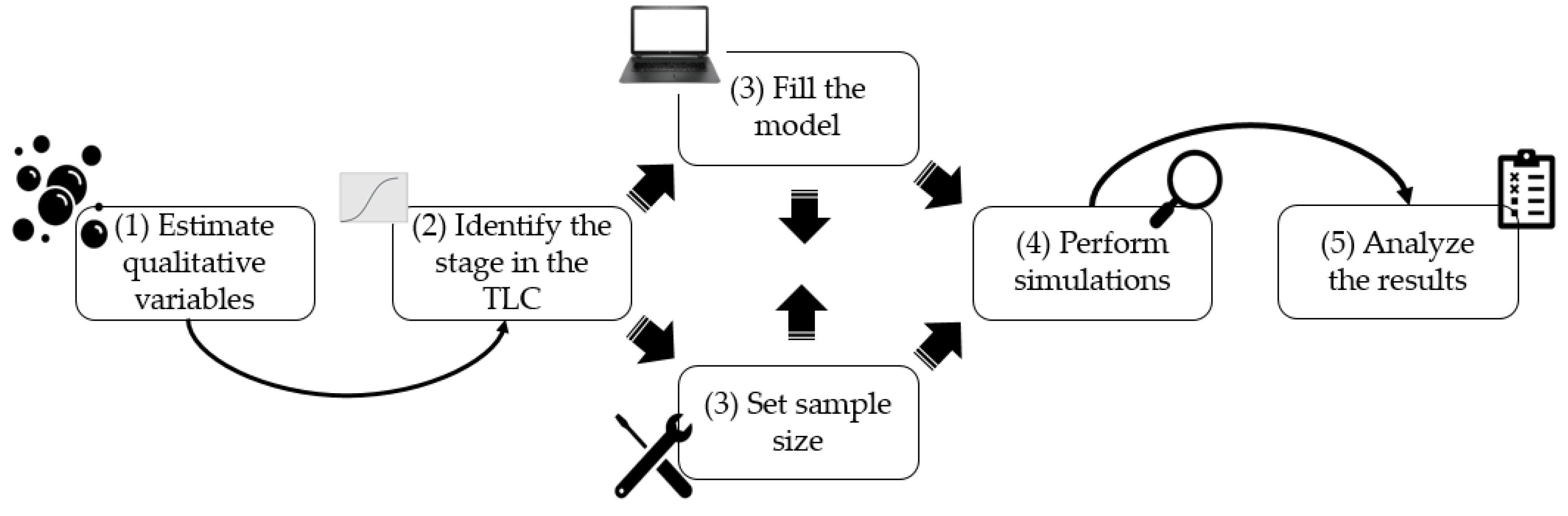
  • Step 1. Estimate Qualitative Variables
In order to estimate the qualitative variables of the model, researchers from the project and representatives from the company were selected to answer the questions previously described in Table 7 to create the respective probabilistic tables. In order to guarantee confidentiality, the answers were anonymous. Table 9 presents the results of the survey conducted with experts.
On the other hand, in Table 10, the a priori variables of TS are shown for the four options of the research form: No, Likely not, Likely yes and Yes, following Equations (2) and (3) previously described.
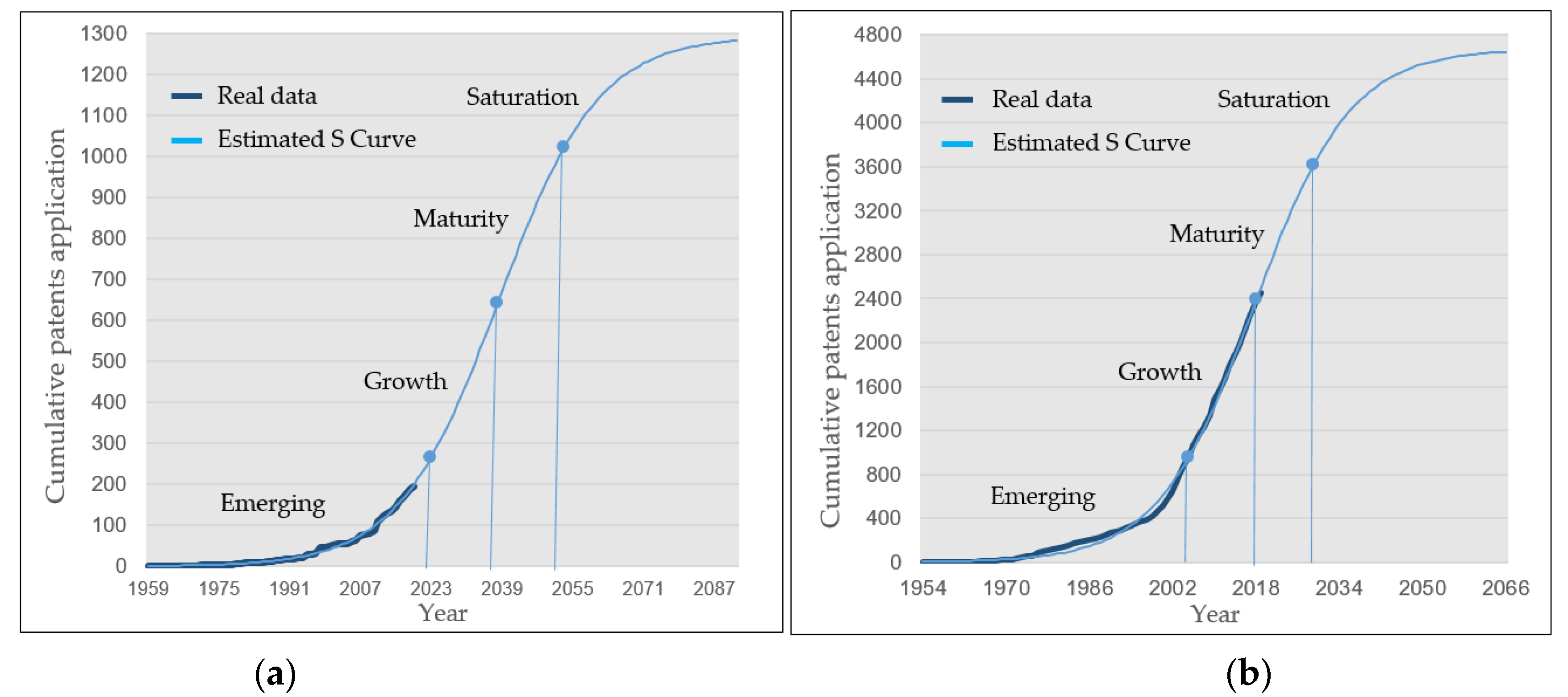
  • Step 2. Identify the stage in the TLC
For the S-curve variable, the steps chosen for TLC analysis and evaluation were based on consolidated references from statistical studies [51,52,53]: data collection, model development and comparison between models, with the use of smoothing methods using growth curves, since these are related to the theoretical basis of S-curves [16,64]. For the data-collection stage, global patent data were obtained, accessed on 17 October 2020 [49], through the use of keywords related to the two aforementioned technologies. The following combinations were used:
  • Cast Iron: (AY >= (1900) AND AY <= (2020)) AND (AB = (grey adj cast adj iron) AND AB = ((sewer adj grate) or (drain adj cover) or manhole or (shaft adj cover*) or cover));
  • Polymeric Concrete: (AY >= (1900) AND AY <= (2020)) AND AB = ("polymer resin" or “polymer” or epoxy or polyester) AND AB = (concrete) AND AB = ((sewer adj grate) or (drain adj cover) or manhole or (shaft adj cover*) or cover).
From the collected data, the model development stage was initiated using an algorithm developed in the R Studio environment [54]. With the obtained data, information from 194 patents regarding cast iron and 2455 patents related to polymeric concrete was imported. As can be seen in Table 11, for both CI and PC, the logistical curve produces the best results for all indicators.
Then, the curves and their respective inflection points were established using Equations (4) (cast iron) and (5) (polymeric concrete), which were obtained from the developed algorithm using the parameters of the logistic curve:
P a t e n t   ( t ) =   1316.8 ( 1.018 + 1292.1 e ( 0.089 t ) )
P a t e n t   ( t ) =   20,176.0 ( 4.32 + 4667.3 e ( 0.1081 t ) )
where ( t ) is time.
Following the concepts explained in Section 3, the second and third derivatives were calculated for each function. Thus, the roots were obtained to determine the inflection points, and the four phases of the S-curve were identified. Subsequently, the graphs in Figure 7 were generated.
The positions of the curves using real data suggest that the PC is in a transition between the phases of growth and maturity (Figure 7b). According to GAO et al. [16], when a technology is in the maturity phase, it tends to become a key technology; it is integrated into products or processes and maintains a highly competitive impact. Therefore, polymeric concrete is approaching an important opportunity to become a key technology in the coming years.
In contrast, CI was expected to be in the maturity or saturation stages since, according to Takata [65], it has been replaced by other materials, such as steel and plastic, in addition to presenting a clear decline in the number of companies that use it. On the other hand, the position on the curve between emerging and growth may indicate a reaction by the CI market as it aims to regain its space by introducing new products and processes, explaining the significant increase in the number of patents published in recent years. This view is also corroborated by the concept of these phases in the S-curve established by [30]: a new technology with low competitive impact and low integration into products or processes.
In this direction, research has been carried out with an aim to promote the optimization of the casting process. Rathore [66] implemented a systematic procedure to analyze defects and then reduce them by optimizing the process parameters. Three parameters were selected to investigate their effects on the final quality: pouring temperature, pouring time and gating system. Advances related to numerical simulations for adequate design for manufacturing, focusing on reproducible quality and cost reduction, were also discussed in the work of [67].
From the perspective of the component, the design optimization of casted products, such as manholes, is also a research focus, as investigated in the work of [68]. This work proposed the optimization of the number of vertical reinforcements by using numerical linear static simulations. Similarly, the authors of [69] proposed an eco-design of the manhole shape through a structural analysis, along with subsequent validation using physical tests and an environmental impact analysis. The results showed the possibility of achieving an approximately 20% mass reduction for one casting, from a weight of 22.60 kg to 18.05 kg.
Based on the data analysis and information from the literature described above, the values in Table 12 were estimated for the model. It is important to point out that the mathematical S-curve model indicates that CI should be between the emerging and growth phases, whereas the literature indicates that it should be in decline. The mathematical and literature predictions for PC are similar. Therefore, an estimate was developed that examined these two outcomes for CI, since the mathematical analysis cannot be dissociated from the opinion of experts [16].
  • Step 3. Enter Values in the Model and Define Sample Size
In this step, two files were created based on the model in GeNIe. The first was for PC and the second was for CI. For each simulated scenario or inference, a text file was generated with 100,000 samples each, generating 8 files with a total of 800,000 samples. The selection of the sample quantity for each simulation was based on an initial simulation to verify the convergence of data, following the law of large numbers [70]. The analysis in Table 13, which used the case study data, shows that as more samples were taken for the same simulation, the results converged. Therefore, a sampling profile of 100,000 was selected for each simulation, as this value generates an absolute error below 0.2% in relation to a sample size of 1 million, as shown in Table 13.
  • Step 4. Perform Simulations
With the data described in the previous steps, four different scenarios were established to perform the simulations:
  • Base scenario 1: Study of the data originally researched and calculated.
  • Inference scenario 2: What if the TRL of PC were equal to 9?
  • Inference scenario 3: What if the TRL and MRL of PC were equal to 9?
  • Inference scenario 4: What if it were possible to develop new formulations for CI that would make imitations more difficult?
It should be noted here that the inferences made were established from the analysis of the original data visualized in the model. This is an important aspect that creates flexibility, since it allows for the analysis of other inferences that may arise if the model is used in other projects.
  • Step 5. Analyze the Results
In this step, simulations carried out from the estimates of the variables previously presented were analyzed, followed by the entry of data into the model to evaluate the options for CI and PC. Based on the characteristics of BN probabilistic models [37], a situation of decision-making under uncertainty was replicated [38] to assist in the selection of options in the PDP. Below, each of the scenarios and inferences are presented by defining their characteristics, displaying the respective graphs and tables and describing the analyses and possible decisions.
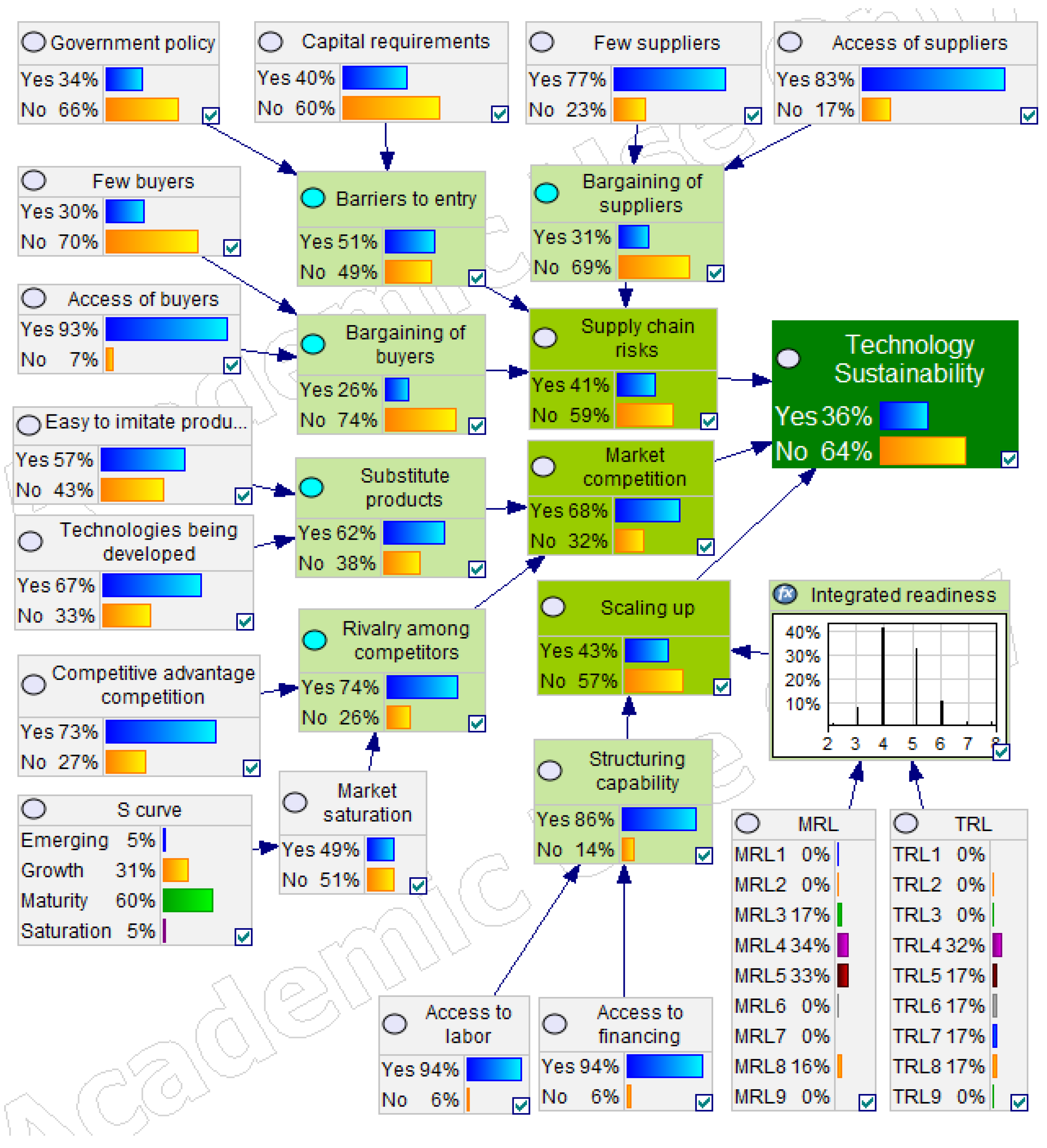
  • Base scenario 1: Study of researched and originally calculated data.
In this base scenario, the obtained results reveal that the probability of TS reaches 50% for CI and 36% for PC. As can be seen in Figure 8, PC presents a critical point when compared with CI due to the low TRL and MRL. This situation is natural, since PC is under development as a product. On the other hand, from the perspective of those who are making the decision of whether to continue the project, it is possible that the performance of PC can improve by increasing the maturity of the technology. Additionally, it appears that the results for both supply-chain risk and the high level of competition are better for PC than those for CI. This fact is very important, as it is possible to choose to continue product development while clearly directing the focus of the efforts to follow. Table 14 summarizes the variables that most influence TS.
Another approach that can be taken from the analysis above is to create a hypothesis regarding what would happen if the TRL and MRL of PC were equal to 9. This new simulation or inference is an important option when using the model, as it allows for the rationalization of cause and effect from the propagation of this change. The intention is to verify the behavior of the two options in a possible combination of scenarios since uncertainty is present in these contexts. Additionally, this combination can provide greater clarity in these moments of decision under uncertainty.
  • Inference scenario 2: What if the TRL of PC were equal to 9?
In the study of this inference, it is observed that despite improving the TS level of PC from 36% to 44%, it is not sufficient to achieve the same result as CI, which is 50% (Table 15). Furthermore, the level of integrated readiness is not sufficient to transform the PC solution into a product ready for the market, as the MRL is still low. Thus, the next inference was made by simulating the scenario in which both the TRL and MRL reach a level of 9.
  • Inference scenario 3: What if the TRL and MRL of PC were equal to 9?
Given the observation of the previous inference, the propagation of changing the TRL and MRL values to 9 was investigated. After the changes, and comparing the results with those of the base scenario, it is observed that the TS dimension increases the probability of being “Yes” from 36% to 55%. In this case, PC appears to be better than CI, the result for which is 50%, as can be seen in Table 16. Hence, a reasonable decision may be to continue investing in the PC project, provided that a strategy is established to overcome the existing barriers to entry. It is also noteworthy that the supply-chain risk, high level of competition and upscaling of technology for PC are improved in this scenario.
Other possible applications for the model include its use as a source of ideas for identifying other weaknesses and defining strategies. Another weakness of PC is related to the current market having few customers, since the probability of this variable being “Yes” is 31%. In order to address this issue, one could examine the feasibility of diversifying customers and, for example, develop a sales strategy for construction companies and condominiums. From there, it is possible to justify proceeding with the project and, at the same time, develop a strategy to access new customers and establish market diversification.
  • Inference scenario 4: What if it were possible to develop new formulations for CI that would make imitations more difficult?
This inference is also important, as it is a mechanism of forming assumptions about the competitor or studying other options in more depth. In this case, it should be noted that the CI product is already consolidated in the market. Table 17 compares CI in this inference with PC that has a TRL and MRL of 9. In this new inference, PC maintains an advantage over CI, with values of 55% and 53%, respectively.
As the values are close, other variables in the model could be used for decision-making, such as access to labor, access to financing and market saturation. Table 18 shows the results of these variables obtained from the simulations for the two options. It is observed that for all variables, PC has a better result than CI. This fact may indicate that with a robust business plan and high TRL and MRL values, PC may be more likely to be sustainable than CI.
Therefore, from the simulations, inferences and analyses carried out, a reasonable decision, provided that it is supported by the final opinions of experts and technicians, may be that it is feasible to continue the PDP of PC. As a condition, it can be stipulated that the TRL and MRL must be enhanced, in addition to establishing customer diversification strategies and a robust business plan that can run in parallel to the PDP of PC. Consequently, the role of such proposed model is to support the decision-making process as the additional fourth dimension in the LCE analysis.

5. Conclusions

The study of sustainability has gradually gained a more holistic and in-depth view. This work followed a methodology that included literature review, development of a model with qualitative and quantitative data and application in a case study. The development of the TS evaluation model makes it possible to overcome important gaps highlighted by Peças et al. [2] in a taxonomy. Thus, is possible to achieve a more complete view by incorporating TS as the fourth dimension into the existing environmental (LCA), cost (LCC) and social (SLC) dimensions in current LCE models. The TS dimension has begun to encompass the technical, market and scale-up perspectives [71], and the maturity phases in the S-curve have been mathematically identified [64]. This model brings a novel approach that encompasses all perspectives in the TS analysis, which was not covered in the literature as described in Table 2. The present study aimed to develop a methodology for measuring TS, and the results showed the following:
  • The use of a hybrid BN makes it possible to encompass quantitative and qualitative variables through the opinion of experts within the context of decision-making in a PDP. Other relevant characteristics of the model are linked to the incorporation of uncertainty related to the use of probabilistic theory. The application of the model in a real project demonstrates its capacity for practical use in both business and academic contexts. Simulations and inferences using the model emphasize its supportive role in the decision-making process.
  • The results of the investigated case study suggest that PC is a potential technology for the production of manhole covers. If efforts are directed toward expanding the maturity of this technology, combined with a strategy to access new customers, the product may perform better than CI, assuming that the other variables remain constant. Even in the scenario involving the emergence of new formulations for CI, PC maintains an advantage over CI.
Therefore, the established model can serve as an analytical tool to facilitate decision making; it is supported by a BN theoretical basis, which makes it possible to effectively deal with uncertainty, with the integration and interdependence of variables and with the combination of quantitative and qualitative data, in addition to making it possible to generate model inferences. All of these aspects can be supported by the analysis and opinions of experts in the context of PDPs, and can be used by companies, researchers and product developers. It is important to highlight that the model can be applied in various circumstances, such as the development of strategies for more sustainable products, selection of more sustainable options and evaluation of competing products. The model can also be adapted, depending on the ease of the software that uses BNs, to allow for the inclusion or modification of variables according to the context of the studies.
However, some limitations need to be discussed. First, the probabilistic tables of nodes had to be estimated since there was no preliminary information. This item can be incorporated into qualitative research as a development stage of the model. Another limitation is related to the application of the model in a single project. Particularly in relation to the research carried out with specialists to assess qualitative variables of technology maturity, a large dispersion of results was observed in variables such as TRL and MRL. Therefore, it is necessary to incorporate criteria that define the profile and experience of the specialists who will evaluate these variables to ensure better consistency between evaluations. For future studies, it is suggested to include other dimensions of sustainability, such as social, cost and environmental factors, in PDPs.

Author Contributions

Conceptualization, A.S.O. and B.A.S.M.; Data curation, A.S.O.; Formal analysis, A.S.O. and B.C.d.S.S.; Methodology, A.S.O., B.A.S.M. and R.S.C.; Project administration, R.S.C.; Software, A.S.O.; Supervision, C.V.F., R.R.S. and R.S.C.; Validation, B.C.d.S.S., C.V.F., R.R.S., B.A.S.M. and R.S.C.; Writing–original draft, A.S.O.; Writing–review & editing, B.C.d.S.S., C.V.F., R.R.S., B.A.S.M. and R.S.C. All authors have read and agreed to the published version of the manuscript.

Funding

This research received no external funding.

Institutional Review Board Statement

Not applicable.

Informed Consent Statement

Not applicable.

Data Availability Statement

The data presented in this study are available on request from the corresponding author.

Conflicts of Interest

The authors declare no conflict of interest.

References

  1. Keeble, B.R. The Brundtland Report: “Our Common Future”, 1st ed.; Oxford University Press: New York, NY, USA, 1988; Volume 4, ISBN 9780192820808. [Google Scholar]
  2. Peças, P.; Götze, U.; Henriques, E.; Ribeiro, I.; Schmidt, A.; Symmank, C. Life cycle engineering—Taxonomy and state-of-the-art. Procedia CIRP 2016, 48, 73–78. [Google Scholar] [CrossRef] [Green Version]
  3. Davis-Peccoud, J.; van den Branden, J.-C.; Brahm, C.; Mattios, G.; de Montgolfier, J. Sustainability Is the Next Digital; Bain & Company: Singapore, Singapore, 2020. [Google Scholar]
  4. Economist, T. Business and Climate Change—The Great Disrupter. Available online: https://www.economist.com/special-report/2020/09/17/the-great-disrupter (accessed on 21 September 2020).
  5. Fernandes, P.T.; Canciglieri Júnior, O.; Sant’Anna, Â.M.O. Method for integrated product development oriented to sustainability. Clean Technol. Environ. Policy 2017, 19, 775–793. [Google Scholar] [CrossRef]
  6. Wulf, C.; Werker, J.; Ball, C.; Zapp, P.; Kuckshinrichs, W. Review of sustainability assessment approaches based on life cycles. Sustainability 2019, 11, 5717. [Google Scholar] [CrossRef] [Green Version]
  7. Kuhlman, T.; Farrington, J. What is sustainability? Sustainability 2010, 2, 3436–3448. [Google Scholar] [CrossRef] [Green Version]
  8. Dong, S.; Li, C.; Xian, G. Environmental impacts of glass- and carbon-fiber-reinforced polymer bar-reinforced seawater and sea sand concrete beams used in marine environments: An LCA case study. Polymers 2021, 13, 154. [Google Scholar] [CrossRef] [PubMed]
  9. Dhillon, B.S.; Balbir, S. Life Cycle Costing for Engineers; Taylor & Francis: Oxfordshire, UK, 2010; ISBN 9781439816882. [Google Scholar]
  10. Jørgensen, A.; Le Bocq, A.; Nazarkina, L.; Hauschild, M. Methodologies for social life cycle assessment. Int. J. Life Cycle Assess. 2008, 13, 96–103. [Google Scholar] [CrossRef]
  11. NASA. NASA/SP-2106-6105 NASA Systems Engineering Handbook; NASA: Washington, DC, USA, 2007; ISBN 3016210134.
  12. Jesus, G.T.; Chagas, J.R.; Milton, F. Integration readiness levels evaluation and systems architecture: A literature review. Int. J. Adv. Eng. Res. Sci. 2018, 5, 73–84. [Google Scholar] [CrossRef]
  13. Sauser, B.; Verma, D.; Ramirez-Marquez, J.; Gove, R. From TRL to SRL: The concept of systems readiness levels. Conf. Syst. Eng. Res. Los Angeles CA 2006, 4, 1–10. [Google Scholar]
  14. Bergerson, J.A.; Brandt, A.; Cresko, J.; Carbajales-Dale, M.; MacLean, H.L.; Matthews, H.S.; McCoy, S.; McManus, M.; Miller, S.A.; Morrow, W.R.; et al. Life cycle assessment of emerging technologies: Evaluation techniques at different stages of market and technical maturity. J. Ind. Ecol. 2020, 24, 11–25. [Google Scholar] [CrossRef]
  15. Sinnwell, C.; Siedler, C.; Aurich, J.C. Maturity model for product development information. Procedia CIRP 2019, 79, 557–562. [Google Scholar] [CrossRef]
  16. Gao, L.; Porter, A.L.; Wang, J.; Fang, S.; Zhang, X.; Ma, T.; Wang, W.; Huang, L. Technology life cycle analysis method based on patent documents. Technol. Forecast. Soc. Chang. 2013, 80, 398–407. [Google Scholar] [CrossRef]
  17. Intepe, G.; Bozdag, E.; Koc, T. The selection of technology forecasting method using a multi-criteria interval-valued intuitionistic fuzzy group decision making approach. Comput. Ind. Eng. 2013, 65, 277–285. [Google Scholar] [CrossRef]
  18. Munthe, C.I.; Uppvall, L.; Engwall, M.; Dahlén, L. Dealing with the devil of deviation: Managing uncertainty during product development execution. R D Manag. 2014, 44, 203–216. [Google Scholar] [CrossRef]
  19. Thomé, A.M.T.; Scavarda, A.; Ceryno, P.S.; Remmen, A. Sustainable new product development: A longitudinal review. Clean Technol. Environ. Policy 2016, 18, 2195–2208. [Google Scholar] [CrossRef]
  20. Tegeltija, M.; Oehmen, J.; Kozin, I.; Kwakkel, J. Exploring deep uncertainty approaches for application in life cycle engineering. Procedia CIRP 2018, 69, 457–462. [Google Scholar] [CrossRef]
  21. Östlin, J.; Sundin, E.; Björkman, M. Linköping university post print product lifecycle implications for remanufacturing strategies. J. Clean. Prod. 2009, 11, 999–1009. [Google Scholar] [CrossRef] [Green Version]
  22. Valerdi, R.; Kohl, R.J. An approach to technology risk management. In Proceedings of the Engineering Systems Division Symposium, Cambridge, MA, USA, 29 March 2004; pp. 1–8. [Google Scholar]
  23. Andrade, H.; Chagas, M., Jr.; Silva, M.; Brito, M.A.; Rocha, D.; Ribeiro, J. Avaliação da Maturidade Tecnológica: Conceitos, 1st ed.; Fbra, E.B.E., Ed.; Edições Brasil and Editora Fibra: Jundiaí, São Paulo, Brazil, 2019; ISBN 9786551040009. [Google Scholar]
  24. Ward, M.; Halliday, S.; Uflewska, O.; Wong, T.C. Three dimensions of maturity required to achieve future state, technology-enabled manufacturing supply chains. Proc. Inst. Mech. Eng. Part B J. Eng. Manuf. 2018, 232, 605–620. [Google Scholar] [CrossRef] [Green Version]
  25. Marlyana, N.; Tontowi, A.E.; Yuniarto, H.A. A quantitative analysis of system readiness level plus (SRL+): Development of readiness level measurement. In Proceedings of the MATEC Web of Conferences, EDP Sciences. Bali, Indonesia, 24 August 2017; Volume 159, p. 02067. [Google Scholar]
  26. Darmani, A.; Jullien, C. Innovation Readiness Level Report—Energy Storage Technologies; REEEM: Stockholm, Sweden, 2017. [Google Scholar]
  27. Munir, M.T.; Mansouri, S.S.; Udugama, I.A.; Baroutian, S.; Gernaey, K.V.; Young, B.R. Resource recovery from organic solid waste using hydrothermal processing: Opportunities and challenges. Renew. Sustain. Energy Rev. 2018, 96, 64–75. [Google Scholar] [CrossRef]
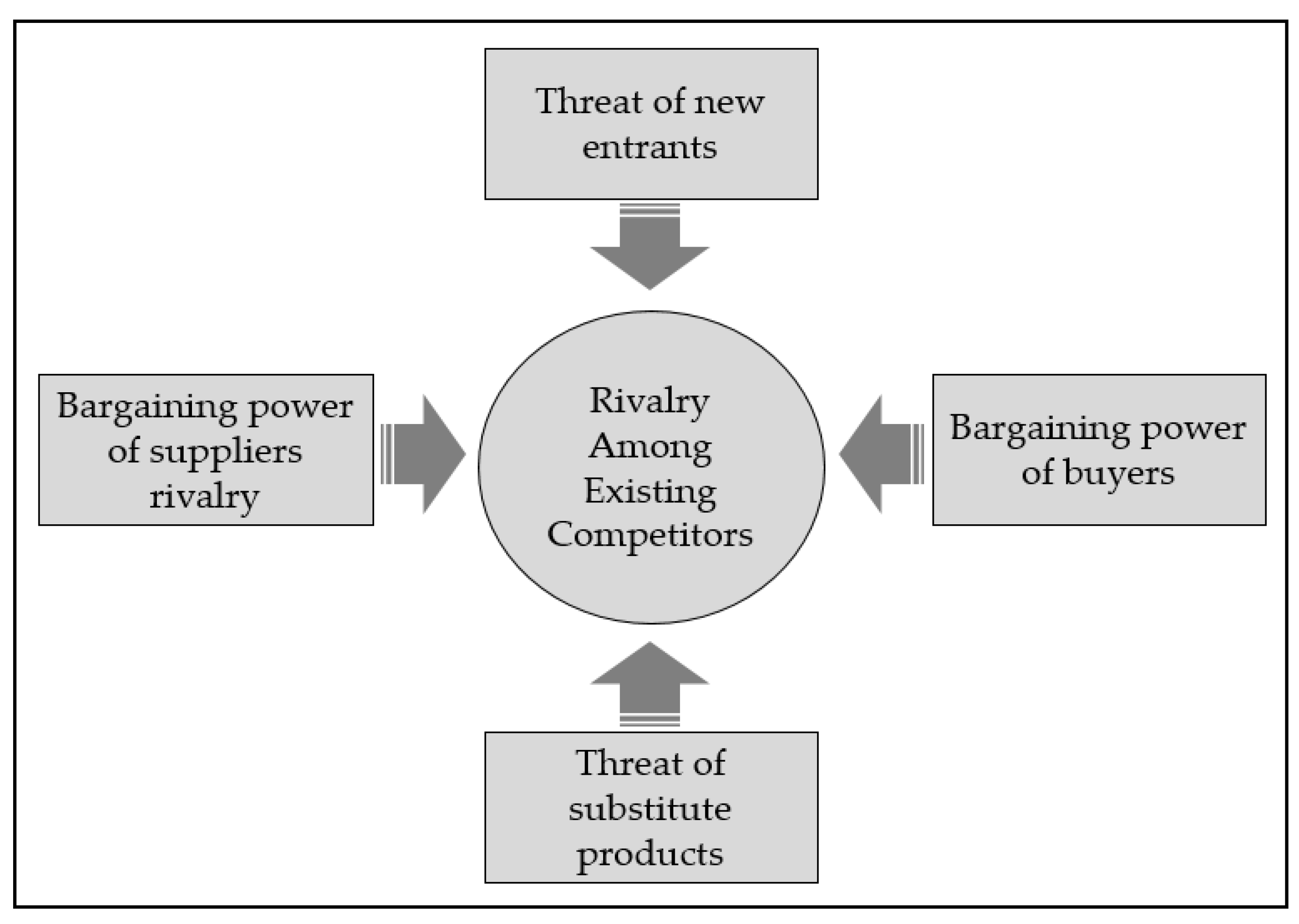
  28. Grundy, T. Rethinking and reinventing Michael Porter’s five forces model. Strateg. Chang. 2006, 15, 213–229. [Google Scholar] [CrossRef]
  29. Porter, M. The five competitive forces that shape strategy. Harv. Bus. Rev. 1996, 1, 23–41. [Google Scholar]
  30. Little, A.D. The strategic management of technology. Eur. Manag. Forum 1981, 1, 1–39. [Google Scholar]
  31. Yang, X.; Yu, X.; Liu, X. Obtaining a sustainable competitive advantage from patent information: A patent analysis of the graphene industry. Sustainability 2018, 10, 4800. [Google Scholar] [CrossRef] [Green Version]
  32. Fye, S.R.; Charbonneau, S.M.; Hay, J.W.; Mullins, C.A. An examination of factors affecting accuracy in technology forecasts. Technol. Forecast. Soc. Chang. 2013, 80, 1222–1231. [Google Scholar] [CrossRef]
  33. Wilder, J.; Sossa, Z.; Palop, F.; Alzate, B.A.; Mauricio, F.; Salazar, V.; Felipe, A.; Patiño, A. S-curve analysis and the technology life cycle: Application in series of data of articles and patents. Espacios 2016, 37, 19. [Google Scholar]
  34. Chang, S.H.; Fan, C.Y. Identification of the technology life cycle of telematics a patent-based analytical perspective. Technol. Forecast. Soc. Chang. 2016, 105. [Google Scholar] [CrossRef]
  35. Madvar, M.D.; Khosropour, H.; Khosravanian, A.; Mirafshar, M.; Azaribeni, A.; Rezapour, M.; Nouri, B. Patent-based technology life cycle analysis: The case of the petroleum industry. Foresight STI Gov. 2016, 10, 72–79. [Google Scholar] [CrossRef]
  36. Caglar, M.U.; Teufel, A.I.; Wilke, C.O. Sicegar: R package for sigmoidal and double-sigmoidal curve fitting. PeerJ 2018, 2018. [Google Scholar] [CrossRef] [PubMed] [Green Version]
  37. Pearl, J. Bayesian Networks; Press, M., Ed.; MIT Press: Cambridge, MA, USA, 2003. [Google Scholar]
  38. Hosseini, S.; Ivanov, D. Bayesian networks for supply chain risk, resilience and ripple effect analysis: A literature review. Expert Syst. Appl. 2020, 161. [Google Scholar] [CrossRef]
  39. Yang, Q.; Li, Z.; Jiao, H.; Zhang, Z.; Chang, W.; Wei, D. Bayesian network approach to customer requirements to customized product model. Discret. Dyn. Nat. Soc. 2019, 2019, 1–16. [Google Scholar] [CrossRef] [Green Version]
  40. Marquez, D.; Neil, M.; Fenton, N. Improved reliability modeling using Bayesian networks and dynamic discretization. Reliab. Eng. Syst. Saf. 2010, 95, 412–425. [Google Scholar] [CrossRef]
  41. BayesFusion GeNIe Academic Version. Available online: https://download.bayesfusion.com/files.html?category=Academia2020 (accessed on 16 September 2020).
  42. McNaught, K.R.; Zagorecki, A. Using dynamic Bayesian networks for prognostic modelling to inform maintenance decision making. In Proceedings of the IEEM 2009—IEEE International Conference on Industrial Engineering and Engineering Management, Hong Kong, China, 8–11 December 2009; pp. 1155–1159. [Google Scholar]
  43. Uusitalo, L. Advantages and challenges of Bayesian networks in environmental modelling. Ecol. Modell. 2007, 203, 312–318. [Google Scholar] [CrossRef]
  44. Li, J. Scaling up concentrating solar thermal technology in China. Renew. Sustain. Energy Rev. 2009, 13, 2051–2060. [Google Scholar] [CrossRef]
  45. Hosseini, S.; Barker, K. A Bayesian network model for resilience-based supplier selection. Int. J. Prod. Econ. 2016, 180, 68–87. [Google Scholar] [CrossRef]
  46. Catlett, J. On changing continuous attributes into ordered discrete attribute. In Proceedings of the Lecture Notes in Computer Science (including subseries Lecture Notes in Artificial Intelligence and Lecture Notes in Bioinformatics), European Working Session on Learning, Porto, Portugal, 6–8 March 1991; Volume 482 LNAI, pp. 164–178. [Google Scholar]
  47. Lima, M.D.C. Método de Discretização de Variáveis Para Redes Bayesianas Utilizando Algoritmos Genéticos; UFSC: Florianópolis, Brazil, 2014; Volume 30. [Google Scholar]
  48. Xiuxu, Z.; Wei, K.; Chuanli, Z.; Benhai, L. Technology life cycle forecasting of chinese hydraulic components based on patent analysis the forecasting of chinese hydraulic cylinder patent development. In Proceedings of the 12th International Conference on Innovation and Management, Wuhan, China, 22–25 November 2015; pp. 1123–1127. [Google Scholar]
  49. Derwent-Innovation Patent Research and Analytics. Available online: https://www.derwentinnovation.com/ (accessed on 9 November 2019).
  50. WIPO WIPO guide to using patent. Available online: https://patentscope.wipo.int (accessed on 20 August 2020).
  51. Kabacoff, R.I. R in Action Data Analysis and Graphics with R; Manning Publications Co: New York, NY, USA, 2011; ISBN 9781935182399. [Google Scholar]
  52. Krispin, R. Hands-On Time Series Analysis with R: Perform Time Series Analysis and Forecasting Using R., 1st ed.; Shetty, S., Ed.; Packt Publishing: Birmingham, UK, 2019; ISBN 9781788629157. [Google Scholar]
  53. Smith, M.; Agrawal, R. A comparison of time series model forecasting methods on patent groups. In Proceedings of the CEUR Workshop Proceedings, Greensboro, NC, USA, 25–26 April 2015; pp. 167–173. [Google Scholar]
  54. Team, Rs. RStudio: Integrated Development Environment for R. Available online: https://rstudio.com/products/rstudio/ (accessed on 10 March 2020).
  55. Petzoldt, T. Growthrates: Estimate growth rates from experimental data. R Packag. Available online: https://cran.r-project.org/package=growthrates (accessed on 20 April 2020).
  56. Kaufmann, K.W. Fitting and using growth curves. Oecologia 1981, 49, 293–299. [Google Scholar] [CrossRef] [PubMed]
  57. Phillips, F. On S-curves and tipping points. Technol. Forecast. Soc. Chang. 2007, 74, 715–730. [Google Scholar] [CrossRef]
  58. Kucharavy, D.; de Guio, R. Application of logistic growth curve. Proc. Procedia Eng. 2015, 131, 280–290. [Google Scholar] [CrossRef] [Green Version]
  59. Conservation, P. Growth II—A Major Upgrade to Our “Simply Growth” Software. Fits and Plots Von Bertalanffy, Gompertz, Logistic and a Wide Range of Other Growth Curves to Length and/or Weight at Age Data; Pisces Conservation: Hampshire, UK, 2006. [Google Scholar]
  60. da Costa, G.A.T.F.; Guerra, F. Cálculo I, 2nd ed.; UFSC: Florianópolis, Brazil, 2009; ISBN 9788599379783. [Google Scholar]
  61. Schot, S.H. Jerk: The time rate of change of acceleration. Am. J. Phys. 1978, 46, 1090–1094. [Google Scholar] [CrossRef]
  62. Huang, L. Growth kinetics of Listeria monocytogenes in broth and beef frankfurters—Determination of lag phase duration and exponential growth rate under isothermal conditions. J. Food Sci. 2008, 73. [Google Scholar] [CrossRef]
  63. Bozdogan, H. Model selection and Akaike’s Information Criterion (AIC): The general theory and its analytical extensions. Psychometrika 1987, 52, 345–370. [Google Scholar] [CrossRef]
  64. Kucharavy, D.; de Guio, R. Logistic substitution model and technological forecasting. Procedia Eng. 2011, 9, 402–416. [Google Scholar] [CrossRef] [Green Version]
  65. Takata, J.T. Análise do Mercado de Fundição dos Metais Ferrosos No Brasil Banca Examinadora; Fundação Getúlio Vargas—FGV: Rio de Janeiro, Brazil, 2002. [Google Scholar]
  66. Rathore, A. Defects Analysis and Optimization of Process Parameters Using Taguchi doe Technique for Sand Casting. Int. Res. J. Eng. Technol. 2017, 4, 432–437. [Google Scholar]
  67. Sturm, J.C.; Schäfer, W. “Cast iron—A predictable material” 25 years of modeling the manufacture, structures and properties of cast iron. In Proceedings of the Materials Science Forum; Trans Tech Publications Ltd.: Bäch, Switzerland, June 2018; Volume 925 MSF, pp. 451–464. [Google Scholar]
  68. Lovrenić-Jugović, M.; Glavaš, Z.; Štrkalj, A.; Slokar, L.J.; Radišić, F. Optimization of the circular manhole cover made of ductile cast iron using finite element method. Mach. Technol. Mater. 2018, 12, 225–228. [Google Scholar]
  69. Cicconi, P.; Landi, D.; Germani, M. An Ecodesign approach for the lightweight engineering of cast iron parts. Int. J. Adv. Manuf. Technol. 2018, 99, 2365–2388. [Google Scholar] [CrossRef]
  70. Hsu, P.L.; Robbins, H. Complete convergence and the law of large numbers. Proc. Natl. Acad. Sci. USA 1947, 33, 25–31. [Google Scholar] [CrossRef] [PubMed] [Green Version]
  71. Trappey, C.V.; Wu, H.Y.; Taghaboni-Dutta, F.; Trappey, A.J.C. Using patent data for technology forecasting: China RFID patent analysis. Adv. Eng. Inform. 2011, 25, 53–64. [Google Scholar] [CrossRef]
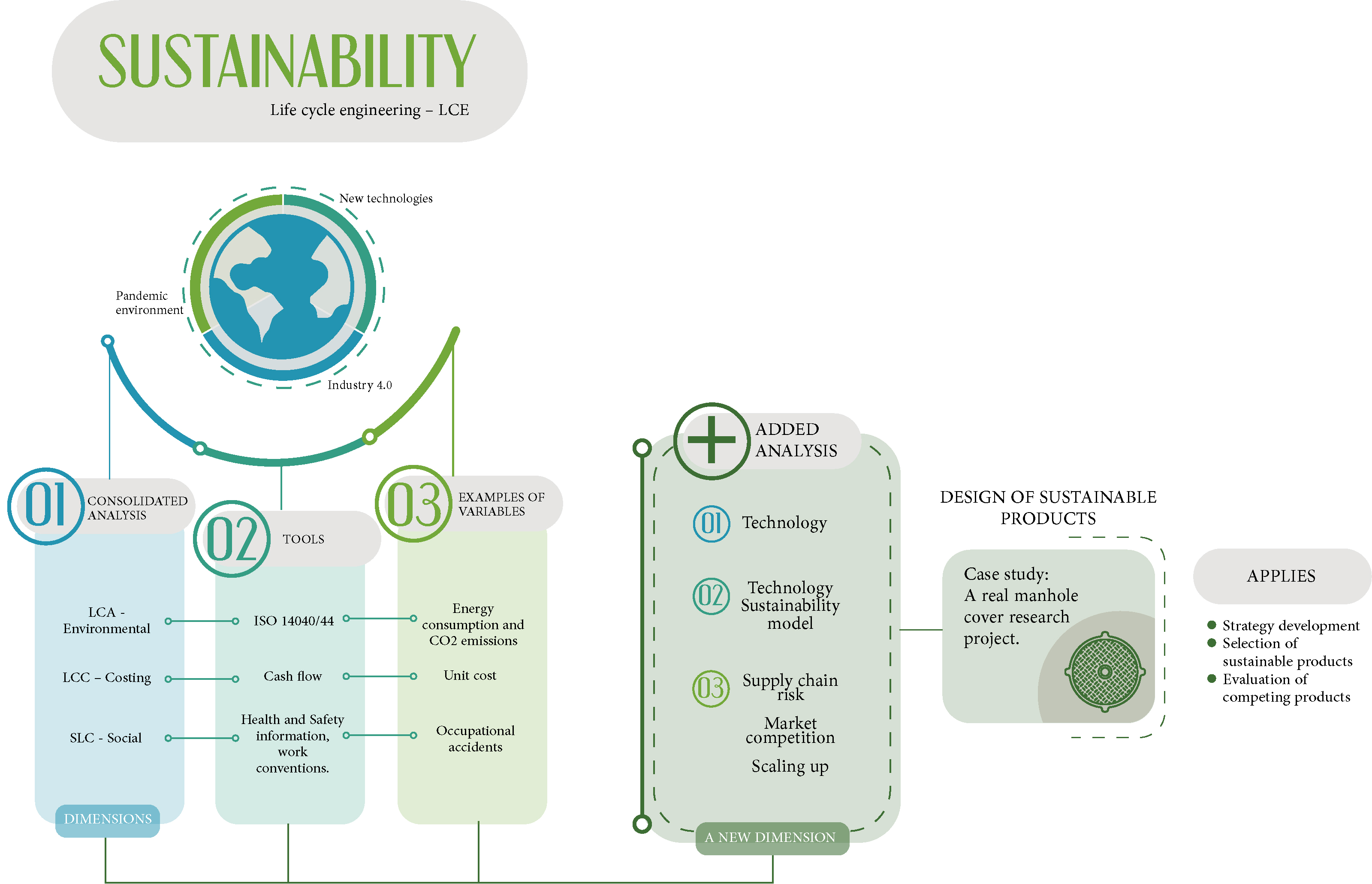
Figure 1. Five forces that shape competition, the relationships between them and the central point of rivalry between competitors. Adapted from [29].
Sustainability 13 02097 g001
Figure 2. S-curve in the technology life cycle (TLC) concept based on patents accumulated over time, presenting the phases of technology maturity: emerging, growth, maturity and saturation. Adapted from [16].
Sustainability 13 02097 g002
Figure 3. Conceptual model of technology sustainability (TS) showing the relationships of the variables of supply-chain risk, market competition and the upscaling of technology and their influences, encompassing the external perspective of the market and the internal perspective of the company applied to PDPs.
Sustainability 13 02097 g003
Figure 4. Probabilistic model in a hybrid BN for measuring technology sustainability (TS), showing the relationships between the variables of supply-chain risk, market competition and upscaling of technology and their influences.
Sustainability 13 02097 g004
Figure 5. Options analyzed in the case study of the Polymeric Concrete project to simulate decision-making in a PDP: (a) reference model with cast iron (CI) and (b) proposed model with polymeric concrete (PC).
Sustainability 13 02097 g005
Figure 6. Steps for using the model: (1) estimate qualitative variables, (2) identify the stage in the TLC, (3) input values into the model and set the sample size, (4) perform simulations and (5) analyze the results.
Sustainability 13 02097 g006
Figure 7. Estimated and real S-curves for the two materials studied in the R&D project, showing the points that were calculated and that separate each phase of the curve’s maturity: (a) CI and (b) PC.
Sustainability 13 02097 g007
Figure 8. Results of the analysis of the base scenario with the model developed in a hybrid BN containing the data of each of the variables and results obtained for (a) PC and (b) CI.
Sustainability 13 02097 g008
Table 1. Current life-cycle engineering (LCE) structure, including dimensions, methods, tools and examples of variables. Adapted from [2].
Dimension and MethodsReferenceToolsExamples of Variables
LCA Environmental[11]ISO 14040/44Energy consumed and CO2 emissions
LCC Costing[12]Cash flowUnit cost
SLC Social[13]Health and safety information; work conventionsAccidents at work
Table 2. Table of methodologies for technology maturity (TM) assessment.
ModelReferenceDescriptionImprovement Points
TRL[11]Evaluates technical readiness and is standardized and recognized by the industry.Reduce subjectivity and expand the scope of the analysis by going beyond the technical aspect.
IRL[12]Evaluates the integration of components in a system.Broaden the scope of the analysis by going beyond the technical aspect.
SRL[13]Combines component readiness and integration.Broaden the scope of the analysis by going beyond the technical aspect.
MRL[24]Evaluates manufacturing.Include market dimension analysis.
SRL+[25]Evaluates the technical aspects in a more global view. Covers the concepts of TRL, IRL and MRL.Include market dimension and technology life cycle analyses.
CRL and SRL[27]Includes customer and societal views of the product.Assess market competitiveness and technical aspects.
Ward et al., 2018[24]Integrates technical analysis, supply chain and life cycle.Include analysis of manufacturing and market competitiveness.
Darmani and Jullien, 2017[26]Evaluates the most external aspects of the market, intellectual property, consumers and society.Assess the technical aspects and obsolescence of technology.
TLC[30]Evaluates the risk and stage in its life cycle. Enables the analysis and anticipation of trends.Analyze the technical and manufacturing perspectives applied to the LCE study.
Table 3. Standardized table for the description of a model variable, adapted from [45].
VariableNPT: Node probability tables that can be represented by estimated tables or formulas.
Description: Reference text to detail the variable, its meaning and reference, if necessary.
Table 4. Details of the TS dimension variables.
Technology SustainabilityUpscalingYesNo
Supply chain risksYesNoYesNo
Market competitionYesNoYesNoYesNoYesNo
Yes25%60%65%95%1%10%20%40%
No75%40%35%5%99%90%80%60%
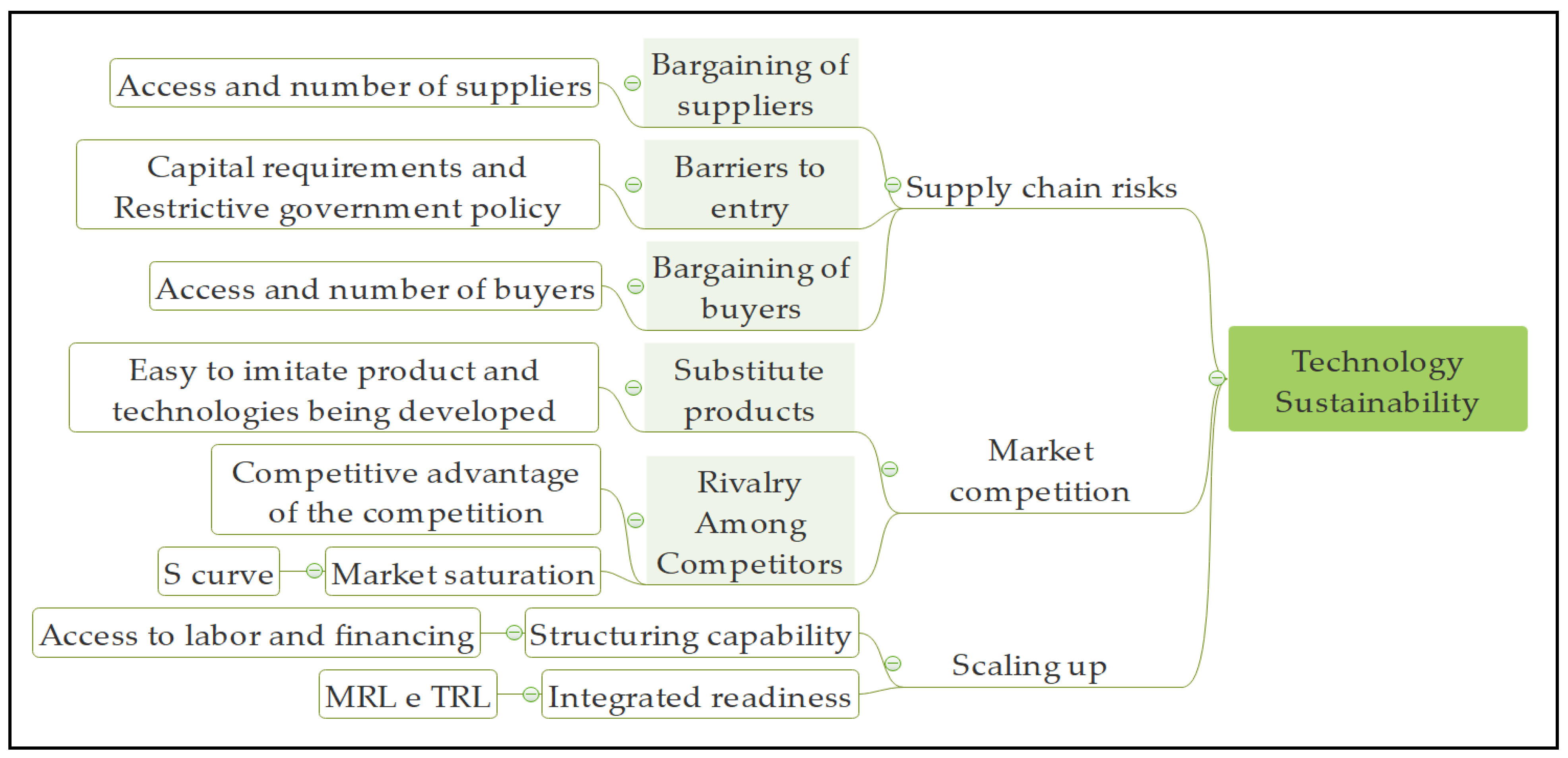
Description: Boolean variable that represents the TS and is affected a priori by the variable of upscaling of technology, and by the variables that consolidate Porter’s Five Forces (supply-chain risks and market competition).
Supply Chain RisksBargaining of supplierYesNo
Barriers to entryYesNoYesNo
Bargaining of buyers YesNoYesNoYesNoYesNo
Yes95%80%85%60%60%40%30%5%
No5%20%15%40%40%60%70%95%
Description: Boolean variable that represents the part related to the supply chain of Porter’s Five Forces and is affected a priori by the variables of bargaining of suppliers, barriers to entry, and bargaining of buyers.
Market CompetitionSubstitute productsYesNo
Rivalry among competitorsYesNoYesNo
Yes95%30%70%5%
No5%70%30%95%
Description: Boolean variable that is affected by the variables of substitute products and rivalry among competitors also referring to Porter’s Five Forces.
Upscaling of the TechnologyIntegrated readiness1–34–67–89
Structuring capabilityYesNoYesNoYesNoYesNo
Yes10%1%40%21%70%41%95%55%
No90%99%60%79%30%59%5%45%
Description: Boolean variable affected by the variables of integrated readiness and structuring capability.
Table 5. Variables that affect the upscaling of technology.
Structuring CapabilityAccess to financingYesNo
Access to laborYesNoYesNo
Yes90%60%40%10%
No10%40%60%90%
Description: Boolean variable affected by the variables of access to financing and access to labor.
Access to FinancingNPT: Yes, No.
Description: Boolean variable to be estimated during the application of the model, using the expert opinion [46,47].
Access to LaborNPT: Yes, No.
Description: Boolean variable to be estimated during the application of the model, using the expert opinion [46,47].
Integrated ReadinessNPT: Readiness_Level = Truncate (((MRL + 1) * (TRL + 1)) ^ (1/2)).
Description: Function-type variable that is affected a priori by the MRL and TRL variables. The Truncate () function was used to ensure that the number was an integer.
MRLNPT: Distributed and estimated among the categories of the variable, i.e., from MRL 1 to MRL 9 [25].
Description: Discrete variable to be estimated during the application of the model, using the expert opinion [46,47].
TRLNPT: Distributed and estimated among the categories of the variable, i.e., from TRL 1 to TRL 9 [11].
Description: Discrete variable to be estimated during the application of the model, using the expert opinion [46,47].
Table 6. Variables of Porter’s Five Forces.
Bargaining of suppliersAccess of suppliersYesNo
Few suppliersYesNoYesNo
Yes10%60%70%90%
No90%40%30%10%
Description: Boolean variable affected by the variables of access of suppliers and few suppliers.
Barriers of entryGovernment policyYesNo
Capital requirementsYesNoYesNo
Yes90%60%70%20%
No10%40%30%80%
Description: Boolean variable affected by the variables of government policy and capital requirements.
Bargaining of BuyersAccess to buyers YesNo
Few buyersYesNoYesNo
Yes60%5%95%85%
No40%95%5%15%
Description: Boolean variable affected by the variables of access to buyers and few buyers.
Substitute ProductEasy-to-imitate productYesNo
Technologies being developedYesNoYesNo
Yes95%60%50%5%
No5%40%50%95%
Description: Boolean variable affected by the variables of easy-to-imitate product and technologies being developed.
Rivalry among CompetitorsMarket saturationYesNo
Competitive advantage of competitionYesNoYesNo
Yes95%70%80%10%
No5%30%20%90%
Description: Boolean variable affected by the variables of market saturation and competitive advantage of competition.
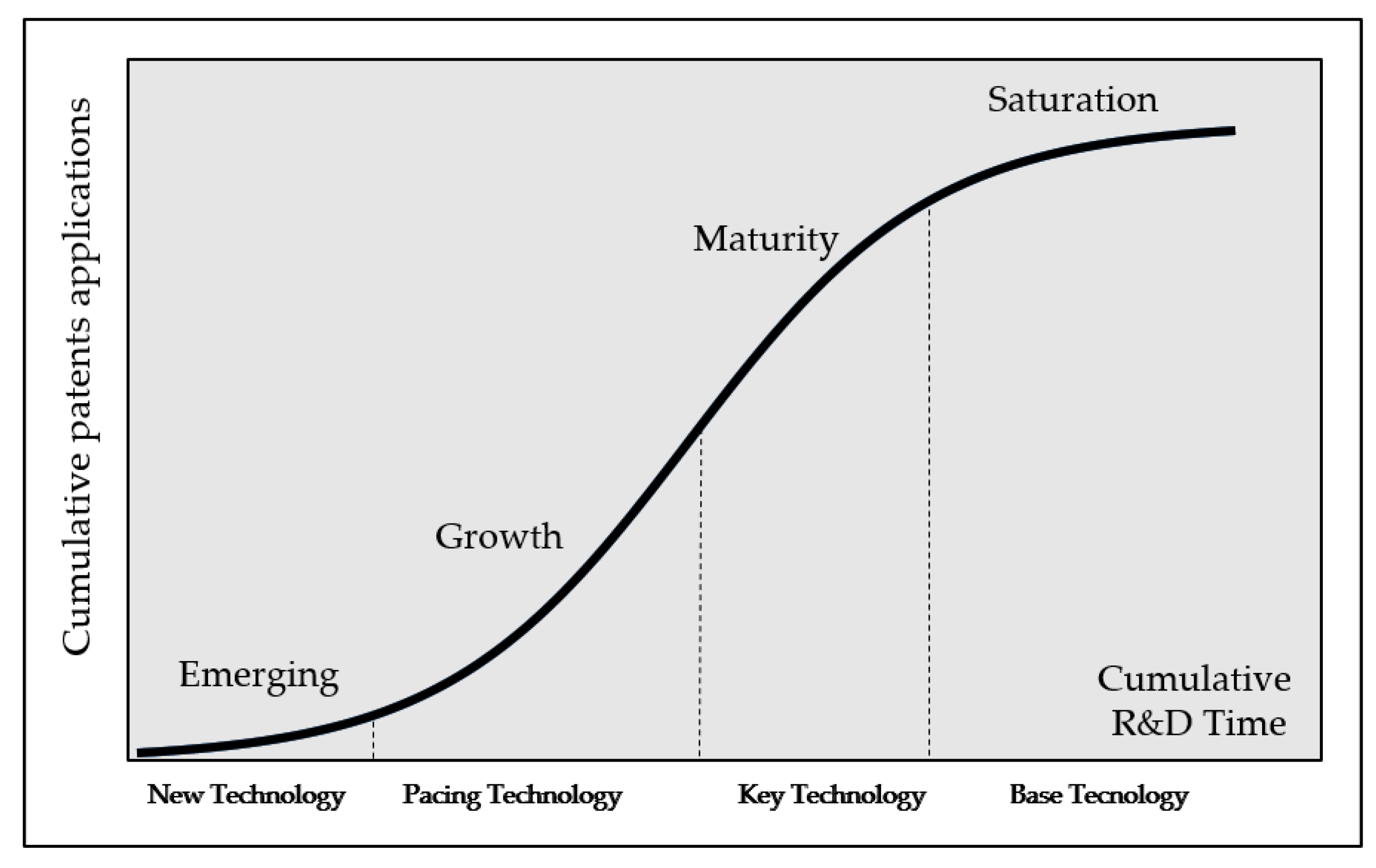
Market SaturationS CurveEmergingGrowthMaturitySaturation
Yes10%30%60%90%
No90%70%40%10%
Description: Discrete variable affected by the S-curve variable.
Table 7. List of questions used to obtain the expert opinion.
Question. Options
1. Structuring capability—Does the sector or company have access to financing (own or third party)?no

likely not

likely yes

yes
2. Structuring capability—Does the sector or company have access to labor?
3. Do the competitors have a competitive advantage?
4. Are there technologies that are being developed and can replace the product under evaluation?
5. Is it easy to imitate or reproduce the product under evaluation?
6. Does the company have access to customers?
7. Does the market have few customers?
8. Do regulations or standards hinder market access?
9. Does it take a lot of capital to enter the market?
10. Does the market have few suppliers?
11. Is it easy to access the suppliers?
11. What is the TRL of the product being evaluated?1 to 9
12. What is the MRL of the product being evaluated?
Table 8. Growth-curve models used in the study.
TypoModelDescription
Growth CurvesLogisticClassic three-parameter growth-curve model [57] used to study and predict future changes [58].
GompertzOriginally used to estimate human mortality, and has three parameters. It can be written in different ways, including four possible parameters (CONSERVATION, 2006).
RichardsA generalization of the logistical curve whose inflection point is no longer symmetrical. It has four parameters [59].
ExponentialClassic two-parameter growth curve [59].
Table 9. TRL and MRL estimates.
Technological LevelCast IronPolymeric Concrete
TRLMRLTRLMRL
10.0%0.0%0.0%0.0%
20.0%0.0%0.0%0.0%
30.0%0.0%0.0%16.67%
40.0%0.0%33.33%33.33%
50.0%0.0%16.67%33.33%
60.0%0.0%16.67%0.00%
70.0%0.0%16.67%0.00%
816.7%16.7%16.66%16.67%
983.3%83.3%0.00%0.00%
Table 10. A priori variables of TS.
VariableCast IronPolymeric Concrete
NOYESNOYES
Access to Financing16.67%83.33%6.67%93.33%
Access to Labor16.67%83.33%6.67%93.33%
Competitive advantage of the competition26.67%73.33%26.67%73.33%
Technologies being developed3.33%96.67%33.33%66.67%
Product is easy to imitate6.67%93.33%43.34%56.66%
Access to Customers3.33%96.67%6.67%93.33%
Few Customers70.00%30.00%70.00%30.00%
Regulation66.66%33.34%66.66%33.34%
Capital Requirement16.67%83.33%60.00%40.00%
Many Suppliers16.67%83.33%23.34%76.66%
Access to Suppliers10.00%90.00%16.67%83.33%
Table 11. Metrics for model selection.
Model(A) Cast Iron(B) Polymeric Concrete
R2RMSEAICR2RMSEAIC
Logistic0.99583.38179.50.996939.2336.3
Exponential0.99563.50179.30.991864.4362.9
Richards0.99553.52183.50.995248.7350.8
Gompertz0.99354.42193.60.988677.7375.6
Table 12. Estimate of the S-curve variable.
EmergingGrowthMaturitySaturation
Cast Iron15%35%15%35%
Polymeric Concrete5%30%60%5%
Table 13. Simulation to define the number of samples.
Number of SamplesTechnology SustainabilityAbsolute Error
10.0%-
1050%50%
10028%22%
100033.9%5.9%
10,00035.0%1.1%
100,00034.8%0.2%
1,000,00034.9%0.1%
Table 14. Values of the variables that most significantly affect TS for PC and CI.
VariablePolymeric ConcreteCast Iron
TRL4–69
MRL4–59
Technology Maturity35%49%
Table 15. Analysis results for a TRL of 9 for CP.
VariablePolymeric ConcreteCast Iron
TRL99
MRL4–59
Technology Maturity44%50%
Table 16. Analysis results for a TRL of 9 and MRL of 9 for PC.
VariablePolymeric ConcreteCast Iron
TRL99
MRL99
Few Customers31%31%
Technology Maturity55%50%
Table 17. Analysis results considering the feasibility of developing new formulations for CI that would make imitations difficult.
VariablePolymeric ConcreteCast Iron
TRL99
MRL99
Technologies being Developed67%96%
Technology Maturity55%53%
Table 18. Comparison between CI and PC.
Polymeric ConcreteCast Iron
Access to Labor93%83%
Access to Financing93%83%
Market saturation50%53%
Publisher’s Note: MDPI stays neutral with regard to jurisdictional claims in published maps and institutional affiliations.

