Abstract
This paper analyses the financial implications, from the point of view of an investor in renewable energy, which sells the energy for an uncertain price of electricity and decides to take advantage of the Colombian tax policy over the renewable energy. The policy, known as Investment Tax Allowance (ITA), encourages installation of renewable projects in a country traditionally dominated by hydro power. Price is modeled as a non-stationary autoregressive stochastic process with normally distributed error terms. Costs, and uncertain revenue and taxes are considered to assess the financial impact on a solar project when the policy is implemented. Since impact varies according to project ownership, two cases are evaluated: a generation company (GENCO-1) that only owns the solar project; and, an existent generation company (GENCO-2) that owns a portfolio of projects. Results indicate that if ITA is applied, it is likely that the GENCO-1 cannot take the full advantage of the incentive, as opposed to the GENCO-2. Although this policy might not satisfy planner objectives since it does not guarantee the construction of significantly high capacity of new renewable energy projects, it definitely represents an attractive mechanism to decrease tax obligations at the GENCO-2 level. Finally, a theoretical analysis shows that investment cost affects the mean of the present value; whereas tax rates impacts both its mean and standard deviation.
1. Introduction
Nowadays, the development of Renewable Energy Technologies (RET) in the world is booming. Two factors that have encouraged this situation are both the establishment of environmental targets and the profitability of RET investments [1,2]. The environmental targets are a direct result of the applicable law [3,4,5,6,7,8], whereas the profitability of RET investments is highly correlated with the constantly declining cost of the investments in the sector [9].
In the last twenty years, numerous incentive policies that promote RET development have been stated and implemented. In the literature, the policies in the field are subject to various classifications [10,11,12,13,14,15]. Feed in tariffs, quota obligations, tax incentives, auctions, and carbon taxes have been the most popular policy instruments declared. In fact, the effectiveness of (the renewable energy generation promotion) policies, measured in terms of RET investment promotion, is subject to the economic development of a country [16].
This research work has focused on the assessment of a recent policy design aimed to promote renewable investments in Colombia via tax incentives. The policy design impact can be sensitive to market conditions such as electricity price uncertainty. The wind power deployment, on one hand, depends on the interaction between electricity price, generation costs, and policy design; on the other hand, it also depends (to a lesser extent) on the policy enactment [17]. A policy design methodology that also addresses tax incentives for biomass co-generation projects is presented in [18].
Energy policy instruments enacted by developed countries have proven to be effective to encourage RET development. Feed in tariffs, tenders and tax incentives in both the European Union and the United States have proved to effectively encourage renewable investments [19]. Also, both fiscal and financial incentives proved to be effective to promote RET in the United States and Brazil [15]. Also, the financial impacts of federal tax credits extensions to promote solar and wind technologies in the United States have been studied [20]. The economic competitiveness of federal tax credits on the development of biomass co-generation, solar photovoltaic and wind power plants in the United States has also been analyzed [21,22,23].
Energy policy instruments that promote RET in developing countries have also been implemented. Two of the most popular instruments to promote RET in Latin American countries have been tax incentives and auction systems [24]. The effectiveness of tax incentives in terms of RET capacity investments have been widely exposed [16,25,26,27].
In Colombia, the RET development energy policy is promoted through the tax incentives provided, according to the Law 1715/2014. The policy provides a set of mechanisms to alleviate the tax burden of RET investors [28]. Among this set of incentives, the policy included value-added tax exclusion and custom tax exemption for certain machinery and services related to RET investments. The policy also allows for modifying the depreciation scheme for RET and created an additional income deduction known as Investment Tax Allowance (ITA). In search of diversifying the Colombian energy mix via RET, the government accomplished its first renewable auction to award a 15-year power purchase agreement [29]. The result of this auction was an allocation of contracts with price agreements of $28/MWh that involve the construction of 1365 MW of RET (7.8% of current installed capacity).
A typical GENCO operating in Colombia sells its electricity production through the wholesale power market and bilateral contracts. In general, the price risk is inherently linked to the nature of the market; however, due to the complex nature of electric energy compared with other commodities, the price volatility represents a key issue [30,31]. Price volatility in Colombia has been dependent on weather conditions [32,33]. According to the Colombian power system operator, 77.6% of national electricity production in 2019 was provided by hydropower plants [34]. Also, during dry seasons, natural gas prices have also influenced market price according to [35].
Given the mentioned market conditions, it results interesting to assess how ITA application combined with long-term electricity price uncertainty actually influences financial feasibility of a RET project in Colombia. As it will be discussed later, the possibility of effectively applying ITA will heavily depend on random taxable income, which is a direct function of market price. Thus, this research focuses on finding out whether or not ITA is an attractive fiscal policy for every RET project and/or investor according to potential income tax savings and present value. Also, this work aims to evaluate the impact of price uncertainty in the financial performance of the project. At the same time, this analysis intends to provide insightful understanding of this fiscal policy to planners, investors, and policy makers. To the best of our knowledge, there are no reported works on modeling effects of ITA in conjunction with electricity price uncertainty so as to explore the potential financial benefits for RET investors. Moreover, a detailed probability distribution of present value of RET shows the factors that really impact the investor’s finances. Additionally, the fact that this type of analysis can become useful for governments, planners, power market participants, and policy makers that pretend to measure the impacts of ITA combined with the market price uncertainty has strongly motivated this research.
Recently, long-term uncertainty in electricity price has been considered to determine the financial feasibility of a RET project. The profitability of an offshore wind installation has been assessed by modeling future electricity prices based on multiple forecasting techniques [36]. Similarly, the uncertainty of hydropower revenue via future electricity prices has been explored [37]. And recently, electricity price uncertainty in the United Kingdom is addressed via Monte-Carlo analysis [38]. Thus, the consideration of electricity price uncertainty is needed to understand both benefits and risks RET investors are exposed to when tax incentives are applied.
Besides Colombia, there are evidences of ITA incentive implementations in other different countries. ITA has also been offered in Belgium, Greece and Spain [39]. Also, Malaysia has designed an ITA mechanism to promote RET development [40,41,42]. A significant segment of the theoretical foundations of our research are based on [22]. Unlike our objectives, it focuses on the analysis of how tax credits—another tax incentive mechanism— affect the levelized cost of electricity (LCOE) of solar photovoltaic projects. The LCOE is nothing but the break-even price of a project, i.e., the electricity unit price at which the project’s net discounted value is zero. The recommended discount rate is the well known Weighted Average Cost of Capital (WACC) [22]. Rather, our research assumes the GENCO sells its energy production at an uncertain market price which does not necessarily guarantee present value breaks-even.
In this article, we analyze implications of applying tax policy, namely ITA, on financial performance of solar PV investors under market price uncertainty. The implications of ITA are analyzed considering a 100 MW solar project from two investors’ perspectives. First, the project belongs to a company which only runs the considered solar project —this perspective is herein after referred to as GENCO-1; in the second situation, the considered solar project belongs to an actual Colombian generation company, which currently runs a portfolio of generation projects —this perspective is herein after referred to as GENCO-2. A detailed development of the present value probability distribution has also allowed to analyze how costs and tax policy impacts the finances of renewable energy investors. In particular, probabilistic indicators of income tax, tax payments, and present are discussed in detail after assuming an autoregressive non-stationary stochastic process for price. A probabilistic analysis of how future tax policies might affect the value added by the project is also performed.
The main contributions of this work have to do with the probabilistic analysis of ITA mechanism established in Colombia. Given the nature of the stochastic process considered for market price, the exact probability distribution model of present value is part of the set of contributions. This result has allowed us to perform multiple tax policy analysis that could eventually assist GENCOs and governments in the decision-making of RET investments.
2. Mathematical Conceptualization of Fiscal Incentives
This section presents the methodology employed to compute the cash stream of a generic GENCO that has invested in a renewable project. In particular, the evaluation will be performed with an especial emphasis on random taxable income, deductions (depreciation and ITA), and tax liability. This cash stream is essential for determining the feasibility of a solar PV project as well as the probability that such a project actually adds value to the GENCO. By doing so, the joint effects of price uncertainty and ITA will eventually assist decision-making processes aimed to determine in which direction expand the generation system of the GENCO. Part of the mathematical models presented in this section is adapted from [22,43].
2.1. Taxable Income
Consider a generic GENCO, owner of an existing generation power portfolio, willing to invest in a renewable energy project. Total taxable income of the GENCO is shown in (1):
where represents additional taxable income in year t gained by selling energy produced by existing generation projects owned by the GENCO. And indicates taxable income of the project, represented by net income before taxes as in Equation (2):
where, is the random electricity price, is the effective number of hours per year the project operates at full capacity C, i.e., . is the capacity factor and is the annual degradation rate [44]. Annual operation and maintenance fixed costs are denoted by . Finally and represent depreciation rate and ITA rate as fraction of project’s investment cost I respectively.
2.2. Rules on Fiscal Incentives
The fiscal incentive policy in Colombia has allowed to apply an annual depreciation rate of up to 20% of the investment cost [28], i.e., , as long as .
The fiscal policy also regulates annual and cumulative application of ITA. Currently, the amount of annual ITA has to be less or equal than 50% of the corresponding taxable income before ITA, as shown in (3):
where represents the annual ITA upper bound for a given electricity price . Likewise, according to [45], the total ITA a GENCO can take advantage of during the first 15 years of project operation cannot be greater than 50% of the initial investment cost of the renewable project, i.e.,
2.3. Income Tax and Net Present Value
Annual tax payments, , are nothing but the local tax rate applied to total taxable income as shown in (4):
and the discounted income tax can be computed as illustrated in Equation (5):
is the discount factor and r is the discount rate.
Also, net present value , computed according Equation (6), is employed to capture the balance between revenue (positive cash flow), and costs and taxes (negative cash flow) over project’s lifetime:
3. Financial Assessment Methodology
This work provides a probabilistic fiscal policy analysis of the impact of the ITA incentive on the financial performance of renewable energy investors. As mentioned before, the stochastic component of this analysis is added by electricity price. The analysis is performed considering electricity price stream as a stochastic process employing a non-stationary autoregressive model. The first approach employed in this assessment is based on simulation of price, and for each realization of price process, taxes and present value are computed using the concepts presented in Section 2. The second approach is a theoretical-based analysis of the probability distribution of net present value, resulting from the propagation of price uncertainty through income tax and present value.
The simulation approach follows the steps illustrated in Figure 1. In year zero, an initial investment is made by a GENCO. Then, for each year, it is necessary to have into account existing taxable income , a particular realization of price , and costs . Both depreciation and ITA schemes need to be designed satisfying the aforementioned fiscal rules presented in Section 2.2. Having applied depreciation and ITA in a feasible way, taxable income and tax liability can also be computed for that particular year. Finally, once lifetime has reached (), income tax and present value can also be determined. Therefore, simulation consists of multiple executions of steps in Figure 1, according to price realizations.
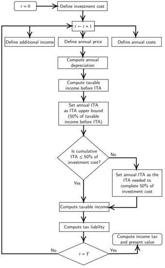
Figure 1.
Flowchart to compute financial implications.
The theoretical approach does not involve price simulation. It directly focuses on the mathematical model of income tax and present value to determine their distributions and statistical properties. This approach is exposed in detail in Section 5.5.
4. Uncertainty in Electricity Market Price
This study assumes the GENCO under consideration sells its electricity production in the power market at a random market price. In the long-term, electricity price represents an important uncertainty for both investors and power market participants in general. Considering a price forecast would not necessarily be an effective approach given the amount of forecast uncertainty in a 20-year plus period. As a result, this research has focused on considering a stochastic process for electricity price with the purpose of evaluate effectiveness of the tax policy through financial performance of a solar PV project.
4.1. Historical Electricity Market Price in Colombia
In Colombia, electricity prices are in fact computed on an hourly basis. Prices represent the marginal cost of the power system operation at every hour and are computed in the generation dispatch process under idealistic conditions after observing actual demand (such as no network congestion) [46].
However, for long-term analysis purposes, annual average historical prices of the Colombian power market have been computed from hourly prices publicly available in [47]. This process is performed for every year in the 2000–2019 period. Data of annual average historical electricity prices and data of ten thousand random samples of future electricity prices are available online in reference [48]. Both data processing and simulation codes were written in R [49].
Also, historical price data, originally recorded in nominal COP/kWh, are indexed to 1 January 2020 COP/kWh using the monthly Colombian producer price index reported in [50]. Once historical prices are expressed in 2020 COP/kWh, the average exchange rate of December 2019 (3383 COP/$) is employed to obtain electricity prices in 2020 dollars ($). Figure 2 illustrates historical the behavior of electricity prices in 2020$. Prices in periods 2009–2016 and 2019 are strongly correlated with the Niño phenomenon as explained by [51,52]. Under Niño phenomenon conditions, the level of reservoirs decrease, which in turn yield to potential scarcity of hydro resources, and subsequent lower hydro production. As a result, the market reaction becomes evident as market price tends to increase due to intensive use of expensive non-hydro technologies [53]. By neglecting the Niño phenomenon intervention on price, a linear trend of price was obtained. The resulting equation is $/MWh, . This represents 0.44% of annual growth in average in the 2000–2019 period. The p-value of the coefficient of the historical price linear trend is 0.291 when Niño phenomenon intervention over price is not considered. In hydro-dominated countries like Colombia, hydropower plants tend to offer every unit of energy at higher prices under scarcity of hydro resources. Thus, if Niño phenomenon data are included in the analysis, the p-value of the linear trend becomes 0.013. That is, price tends to increase over time.
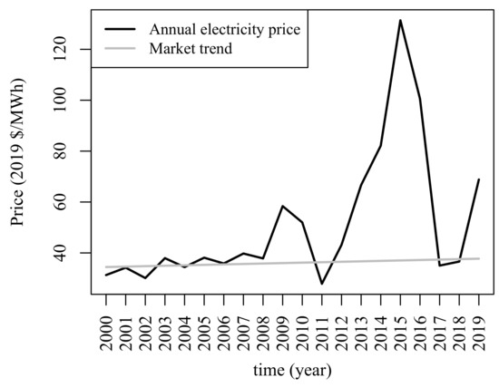
Figure 2.
Electricity price and market trend in constant 2020 dollars from 2000 to 2019.
4.2. Stochastic Process Model for Electricity Price
An AR(1) model has been also considered in order to represent uncertainty of electricity price some degree of correlation in the price process on a yearly basis. Average annual price is modeled as shown in Equation (7):
where error terms are i.i.d. and represents unbiased normal perturbations. This analysis has been constructed employing and . corresponds to the average price of year 2019 equal to 37.73 $/MWh. When standard deviation of electricity price at year 1 (parameter ) is significantly high (generally above ), year-20 prices might become negative although with low probability. This situation would be unrealistic. In addition, considering to be around guarantees random prices can be high enough to capture potential price spikes due to Niño phenomenon as Figure 3 illustrates. Figure 3 shows 500 realizations of prices under approach. The trajectory of expected price, given by , is represented by the solid black line. It basically displays a 2% annual increase on average and is defined by . According to the random trajectories, it is also noticeable price variance, modeled through Var increases over time. Theorem A1 and Corollary A1 in Appendix A present the theoretical development of the parameters of electricity price distribution.
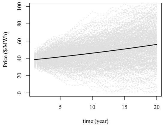
Figure 3.
500 random price trajectories.
Figure 4 displays the resulting autocorrelation function of the price process considered in this paper. A theoretical development of such a function is presented in Corollary A2. An important fact to highlight is that, due to non-stationarity, is not a function solely of time lag , it is actually a function of t and . That is, .
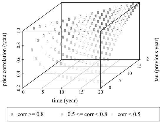
Figure 4.
Autocorrelation function of price .
As expected, . In fact, the smallest correlation observed is , which does not suggest linear statistical relationship among such prices. However, highest correlations occur as long as time evolves according to Figure 4.
5. Numerical Results
In this section, we analyze financial implications of using ITA under electricity price uncertainty, on financial performance of two GENCOs that are willing to invest in a 100 MW solar PV facility. The first GENCO, referred to as GENCO-1, is an agent that only owns the solar project; and, the second GENCO, referred to as GENCO-2, is an exiting agent owner of a generation power portfolio. In particular, company Urrá is our GENCO-2, a 99.9% state-owned GENCO located in Tierralta, Córdoba in North-West Colombia [54]. Average peak sun hours in this region is 4.45 h/day [55]. Currently, this GENCO runs a 340 MW hydropower plant and provided 1.85% of Colombian electricity production in 2019 [46]. The reader can refer to [56] for additional information regarding this company.
5.1. Input Parameters
This financial evaluation considers the idea that Urrá plans to invest in a 100 MW solar PV project. The investment cost of this type of project can still be close to $1000/kW [57]. However, recent works like show that it can be $756/kW [58], which adds up to $75,600,000 for the project under analysis. Fixed operation and maintenance cost is $10.5/kW-yr, which represents $1,050,000/year for the project. The degradation rate used in this analysis is 0.05% [44], which indicates project’s production capacity is reduced annually in such a fraction. Finally, the capacity factor imputed to this project is 19% [55]. In other words, the initial production is 19% of the project’s rated energy production. The initial rated energy production is 876,000 MWh/year (100 MW × 8760 h/year).
In addition, future cash flows are analyzed using a discount rate of 5% [59]. In terms of taxes, this work adopts the maximum yearly depreciation of 20% during the first five years of project operation established by tax regulation. Also, legislation has adopted a tax rate of 33%, which applies over taxable income [60].
5.2. Policy Analysis at the GENCO-1 Level
The objective of this section is to analyse how the fiscal policy, under electricity price uncertainty, affects the finance of the GENCO-1 (solar project). To do so, we start by defining an ITA scheme that is ultimately compared to a situation where the ITA incentive does not apply.
5.2.1. Fiscal Strategies
The analysis is developed by illustrating different possible forms of applying ITA. To compute the project’s taxable income , an “intensive” ITA scheme has been designed. This scheme deducts annual taxable income as much as possible. In other words, this ITA scheme is set as the annual upper bound, defined in Equation (3), as long as cumulative ITA falls below $37.8 million (50% of the initial project’s investment cost).
Therefore, the “intensive” ITA scheme, denoted as , can be computed as
Given the uncertainty in electricity price captured in the set of scenarios, ITA intensive scheme is also uncertain since it depends on energy sales revenue, which in turn is a function of uncertain price . The resulting period of ITA application, denoted as , is therefore the last year in which , i.e.,
Note that in year , ITA cannot be necessarily at its upper bound. Rather, it is chosen to complete the 50% issued by the Colombian regulation. Figure 5 presents trajectory distributions of the intensive ITA application given the uncertain electricity price process. Whenever years, it results impossible for the GENCO-1 to take advantage of any ITA at all given that . Thus, ITA is applied anytime from year 6 up to year 15 as legislation states. In this time frame, ITA is rarely greater than 8% annually. In fact, ITA is about 4% annually in average. Although with low probability, there are some extreme cases, when price is really low, in which ITA cannot be applied in some particular year.
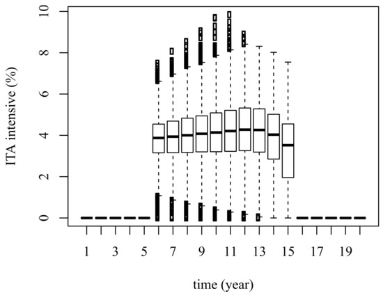
Figure 5.
ITA intensive for GENCO-1 (solar project).
The distribution of the cumulative (or total) ITA application in this project is displayed in Figure 6. Due to hard constraints on annual ITA application, combined with price uncertainty, it is likely to have situations that impede the GENCO-1 to make use of full tax incentive. It indicates that it is more likely to have situations that cannot take advantage of the ITA incentive. The total ITA offered by the government seems to be still low for solar PV projects. According to these results, there is a probability of only 27% that a particular solar PV project can fully absorb the 50% ITA granted by the government.
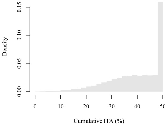
Figure 6.
Cumulative ITA for GENCO-1 (solar project).
5.2.2. Taxes
As a consequence of the execution of the fiscal strategy just described, tax payments are significantly influenced. Figure 7 presents the trajectories of under presence and absence of ITA. Tax obligations, in both cases, are negative as long as years, i.e., during period of heavy depreciation amounts (20% of investment cost annually). Negative taxes represent tax losses and are modeled as positive cash flows for computing present value. Once depreciation is completed, taxable income becomes positive and ITA can be applied. In fact, during the period years, annual tax obligations reductions oscillate between $0.79 million and $1.06 million in average as presented in Figure 7. On the other hand, if ITA is not employed, annual taxes are close to $2 million after applying depreciation. Figure 7 shows evidence of significant tax reductions as a result of the tax incentive.
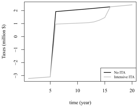
Figure 7.
Trajectories of for GENCO-1 (solar project).
The resulting distribution of income tax for the project is presented in Figure 8. In average, under ITA absence, million; however, taking advantage of the incentive, million. In fact, the probability that the project ends up with negative income tax increases from 29% to 69.1% when ITA is considered. That is, the probability that the tax authority effectively collects taxes is only 30.9% from new firms under the incentive mechanism.
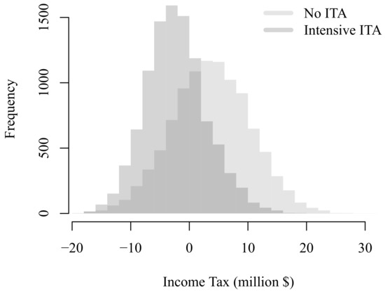
Figure 8.
Income tax for GENCO-1 (solar project).
5.2.3. Value of the GENCO-1
Finally, the value of the project is also affected by price uncertainty. Figure 9 displays the distributions of under absence and presence of ITA. Project’s value is normally distributed with known parameters when ITA is not considered. These parameters are carefully described in Appendix B. But, when the uncertain intensive ITA is applied as defined in Section 5.2.1, it adds additional randomness according to (7) to the cash stream and thus no longer follows a normal distribution.
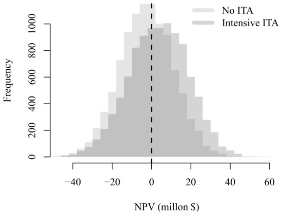
Figure 9.
Distribution of for the GENCO-1.
As expected, when ITA is applied, average value increases from −$2.55 million to $3.45 million. That is, ITA adds value in average to this type of solar projects. Standard deviation increases from $13.59 million to $15.10 million once ITA is implemented given the additional uncertainty added by such a tax deduction. In probabilistic terms, the probability of having negative value decreases from 57.1% to 40.7%. Although project’s value distribution has shifted towards positive numbers, this kind developers can still represent a risky investment for either new or small companies. Additionally, according to the highly likely situation of obtaining negative income tax, as illustrated in Figure 8, part of present value represents tax losses.
In general, a tax loss represents money that can be employed in the future to offset future tax obligations. However, tax regulation of each country establishes requirements to companies for its use [61]. For instance, Austria, Brazil, France, Italy, Japan, Portugal, Russia, and United States limit the use of tax losses up to a given percentage of taxable income. Some countries like China, Germany, Netherlands, Norway, Spain, Sweden, Switzerland, United Kingdom, and Colombia do not impose such a constraint. Tax regulation in Colombia, China, Netherlands, Switzerland, Japan (and other countries) establishes a maximum period in which tax losses can be used. In particular, Colombia allows tax losses to offset future tax obligations in a 12-year period [62]. This work has considered tax losses are once taxable income become positive.
5.3. Tax Policy Analysis for the GENCO-1
The role played by ITA and tax rate in the tax obligations of the project is interesting. Consider an alternative formulation of the net present value as the one given in Equation (10):
where is the discounted gross revenue of the project, and represents the discounted taxable income of the project (not GENCO’s) and defined as:
Under usual circumstances, an investor manages its project with the purpose of achieving positive value. In fact, the investor undoubtedly would do his/her best in order to achieve positive taxable income ; and will rationally prefer the government not to increase tax rate and thus not worsen project’s value. However, after inspecting Equation (11), high values of ITA, combined with relatively low prices, can reduce discounted taxable income. Even more, can become negative, i.e., the project incurs in tax losses. In such a case, the investor’s attitude with respect to governmental tax policy suddenly shifts: the investor is better off as long as tax rate increases. This is explained by the fact that for some special conditions that will be discussed below.
In this analysis, is also a random variable given electricity price uncertainty. Also, discounted taxable income strongly depends on initial investment cost I and depreciation plan as suggested by Equation (11). Figure 10 represents the distribution of , i.e., the negative of the random sensitivity of with respect to tax rate for the project. According to this work, discounted taxable income decreases from $11.33 million to −$6.84 million in average once ITA is implemented. Therefore, if real price ends up close to its expected value, this project would benefit anytime government decides to increase tax rate. But, in this experiment, increases from 29.02% to 69.14% when ITA is actually applied. It is surprisingly likely this project ends up collecting tax losses and taking advantage from possible government tax policies that tend to increase tax rates.
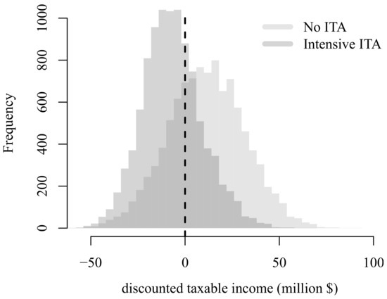
Figure 10.
Discounted taxable income ().
5.4. Policy Analysis at the GENCO-2 Level
Now, the analysis focuses on understanding the financial impact of ITA over an existent GENCO that decides to build the solar project. As mentioned earlier in this paper, Urrá is our GENCO-2, a 99.99% state-owned company that currently operates a 340 MW hydropower plant in Northern Colombia.
Formulation presented in Section 2.1 presumes a GENCO that owns a portfolio of existing generation projects, which will in turn continue providing an additional taxable income labeled as . In order to perform an accurate analysis, was extracted from Urrá’s financial statements, which includes before-tax and after-tax profit data, among others. Interested readers in Urrá’s financial details can refer to [63,64]. Figure 11 illustrates historical Urrá’s taxable income and its trend from 2013 to 2018. Its high variability is mainly associated with energy transactions in the power market at variable prices. The trend, in 2020 dollars, is employed to estimate the stream of .
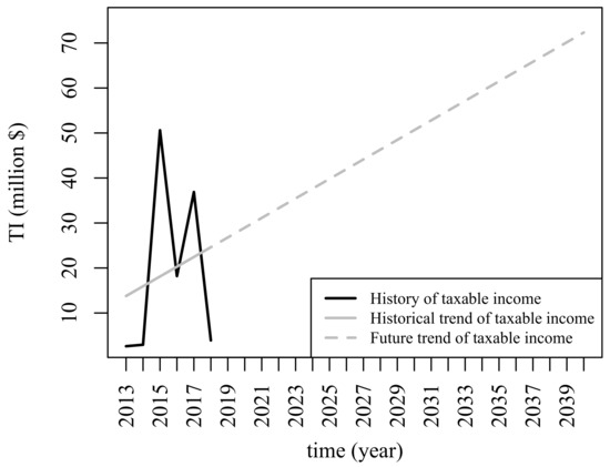
Figure 11.
Urrá’s financial statements in 2020 dollars.
5.4.1. Fiscal Strategies
In this case, we illustrate two different possible schemes of applying ITA: “uniform” and “intensive.” The first one allows ITA to be 10% annually over a 5-year period. That is, Urrá would take 10% of project’s investment cost as an additional annual tax deduction. In 2020 dollars, this represents an ITA of $7.56 million annually as long as years. The “intensive” ITA scheme focuses on deducting taxable income as much as possible every year adopting the same approach explained in Section 5.2.1.
Figure 12 summarizes the uncertain application of the “intensive” ITA scheme price given electricity price uncertainty scenarios. In every scenario, years; however, the amount the GENCO can deduct as ITA is variable. Note that in year , ITA cannot be necessarily at its upper bound. Rather, it is chosen to complete the 50% issued by the Colombian regulation. In this case, total GENCO’s taxable income becomes , which permits to relax the ITA constraint by increasing its annual upper bound shown in Equation (3). ITA gradually increases during the first three years from 14.1% to 17.1% in average; then at , it reduces to 3.1% in average with the purpose of taking advantage of the total 50% offered by the government.
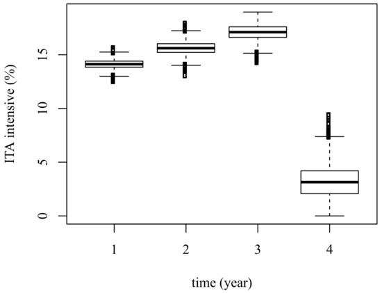
Figure 12.
Application of ITA intensive for GENCO-2.
The effects of were both to enable the GENCO taking advantage of ITA once the projects starts operation and to reduce ITA application period . This second effect would in turn represent additional benefits—measured in terms of tax savings—for this GENCO. On the contrary, the GENCO-1 whose would have to apply ITA according to results analysed in Section 5.2.1. Based on these findings, this incentive seems to work, as intended, for companies that also perceive an additional income sufficient enough to enable application of ITA in a more effective fashion.
5.4.2. Taxes
As a consequence of the execution of the fiscal strategies explained previously, tax payments can be significantly influenced. Figure 13 present the trajectory of . Taxable income as well as tax obligations for Urrá are always positive given its relatively high income from other projects. Differences between ITA schemes are noticeable as long as years, period in which of both depreciation and ITA apply. In absence of ITA, initial mean tax payments start from $7.05 million; if ITA is taken, tax payments reduce to $4.55 million and $3.52 million in average for ITA uniform and intensive respectively. Later, once tax deductions have been completely applied, the effect of the incentive mechanism vanishes.
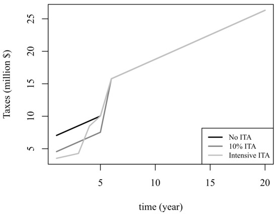
Figure 13.
Trajectories of for the GENCO-2.
The sooner the GENCO apply ITA the higher tax savings obtained. Given the time value of money captured by the discount rate, it results more attractive to delay tax payments as much as possible.
Resulting income tax distributions for different ITA schemes are shown in Figure 14. Also, the solid black vertical line represents Urrá’S income tax if it decided not constructing the solar project, and can be computed as million. On the other hand, if the project is actually built without applying ITA, average income tax would be $202.22 million, and $191 million if is applied intensive ITA scheme. In other words, constructing the project applying ITA would imply $7.48 million of average tax savings. Additionally, the probability Urrá ends up saving taxes by constructing the project and applying ITA is approximately 86.9%. If ITA is not applied, the probability decays to 29%. These kind of results provide crucial signals that lead any GENCO to appropriate RET investment decisions.
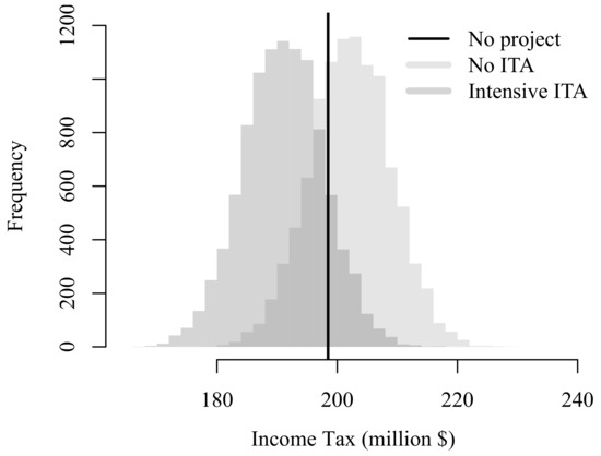
Figure 14.
Income tax for the GENCO-2.
5.4.3. GENCO-2’s Value
The present value is analyzed through Figure 15. It shows the distribution of under absence and presence of ITA (under the intensive scheme). Also, a solid black line indicates present value of the GENCO-2 even if this solar project is not built. It is computed as the discounted after-tax income, i.e., million. According to these results, it looks that this project adds value to the GENCO-2 only if ITA is implemented. Indeed, average present value is $400.44 million (<). But, it increases to $411.66 million (>) when ITA is applied. Standard deviation of present value slightly increases from $13.59 millions to $13.61 millions as long as ITA is applied.
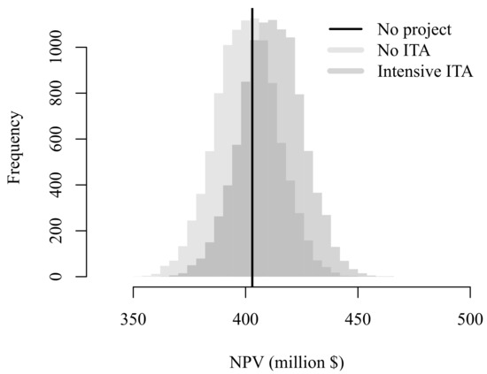
Figure 15.
Distribution of for the GENCO-2.
In brief, only when ITA is available, present value distribution would be very likely to be greater than current GENCO-2 value . In fact, the probability that present value overpasses $402.98 million is just 42.87% if ITA is not implemented; whereas, the same probability increases up to 73.63% when the GENCO-2 takes fully advantage of the intensive ITA mechanism. Also, if ITA is slightly reduced and taken in portions of 10% during five years, the probability that the project adds value to the GENCO-2 is 73.17%. Therefore, it can be said that the risk, measured as the probability that the project does not add value to the GENCO-2, is around 26%, according to our experiment and assumptions.
Unlike the case of the GENCO-1 analyzed in Section 5.2, tax losses are not registered in the case of this GENCO-2. Tax losses heavily depend on the financial performance of additional projects owned by the GENCO-2. Projected taxable income of existing projects registered by Urrá, depicted in Figure 11, are sufficient to enable a quick use of the ITA incentive (usually in four years). A GENCO-2 with much higher income could enjoy additional economic benefit by applying total ITA even in the first year of project operation.
5.5. Distributional Analysis of Economic Value
A series of theoretical results regarding the distributions of price and present value are discussed in Appendix A and Appendix B. Theoretical results hold for the AR(1) model employed for the electricity price process when ITA is employed in a deterministic fashion. Intensive ITA scheme is therefore no longer analyzed in this section since it depends on random taxable income.
When random errors of the AR(1) process are independent and normally distributed, price is normally distributed (Appendix A), therefore present value is also normal. Motivated by a series of distributional facts, this section (Appendix B) presents a theoretical analysis about the influence of investment cost and tax rate on the resulting distribution of present value from the GENCO-2’s standpoint. Figure 16 shows the theoretical distribution of GENCO-2’s under deterministic changes in solar investment cost I. As observed in Appendix B, only depends on I, whereas does not. This translates into different scales of distribution. As expected, decrease in investment cost shifts right present value.
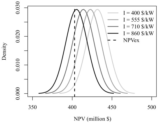
Figure 16.
Distribution of GENCO-2’s as a function of investment cost I.
Figure 16 also represents , when million as a reference value to consider whether or nor the solar project is a sound decision. A particular GENCO-2 would justify its decision according to the probability that its value with project is greater than its value without project for some particular investment cost I. An exact computation of such a probability can be performed using Equation (12):
where is the cumulative distribution function (CDF) of the standard normal distribution, and given by
Parameters and denote the mean given a particular investment cost I and variance of present value respectively as shown in Theorem A5 in Appendix B.
Apart from investment cost, it was found that tax rate really affects the financial performance of the project. Figure 17 shows the theoretical distribution of GENCO-2’s under different tax rates. As observed, both scale and form are significantly affected by . Unlike expected present value, uncertainty of GENCO-2’s tends to increase as long as tax rate increases. As discussed in Appendix B, price uncertainty is scaled by and this factor finally spreads to present value. According to our assumptions, standard deviation of GENCO-2’s ranges from $17.2 million to $9.1 million when is increased from 15% to 55%. The greater , the lower uncertainty.
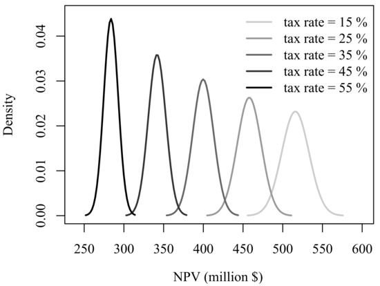
Figure 17.
Distribution of GENCO-2’s as a function of tax rate .
The fact that tax rate also affects makes necessary to analyze, from a probabilistic standpoint, whether or not the solar project adds value to the GENCO-2. By using Equation (12), it is possible to compute how likely the solar project adds value to the GENCO-2. Figure 18 illustrates multiple changes of with respect to tax rate and investment cost. As expected, low investment cost reduces total costs and favors . However, it is more likely that the project adds value to the GENCO-2 as long as tax rate increases.
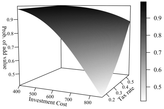
Figure 18.
as a function of I and .
If government increases tax rate, two opposite effects are encountered. First, the value of the GENCO-2 due to existing projects is actually reduced, which facilitates the observation of . And second, the fiscal incentive applied to the solar project allows paying low taxes at the company level, which in turn translates into higher total value. This last effect is predominant for the GENCO-2 subject to this study; and thus the resulting combined effect establishes that it is more likely for the GENCO-2 to perceive additional value if tax rate is increased. From Figure 18, one can observe that no matter what the investment cost is, the probability of adding value exhibits an increasing tendency with tax rate. And it is significantly high when investment cost is low. It is important to highlight that a high probability of adding value does not necessarily imply a high probability of achieving high .
6. Conclusions
This paper focused on assessing the impact of electricity price uncertainty and a fiscal policy based on ITA, established by the Colombian government, on RET investments. To do so, we create a financial performance assessment methodology for a renewable energy investor—willing to invest in a RET project—based on a probabilistic analysis of both income tax and present value.
Electricity price uncertainty is simulated through a non-stationary autoregressive model AR(1). This approach has allowed to obtain analytical results when ITA is employed in a deterministic fashion. Random ITA applications have required simulating price uncertainty considering multiple scenarios. Thus, income, taxes (and tax deductions), and present value are heavily affected by price uncertainty. All of this has been studied over a 100 MW solar power plant constructed by both GENCO-1 and GENCO-2.
The effectiveness of the fiscal policy, measured in terms of quantity of potential developers of RET projects, is really affected by cash flow uncertainty. Annual ITA upper bound criterion imposed by the tax policy, can be even zero if future low-price situations unfold. Thus, many potential projects might end up getting low financial benefits. As a consequence, the probability that projects can effectively take advantage of the total 50% ITA (awarded by the policy in the 15-year period) is low. Therefore, as a consequence, the current state of this tax policy might not be enough to satisfy planner objectives in the sense that it cannot guarantee a sufficient capacity of renewable energy projects.
Taxes collected by the government from either GENCO-1 or GENCO-2 can be really uncertain. It was observed that this situation is evident as long as the GENCO-1 takes advantage of ITA. Not all of them end up paying taxes and their income tax can become negative, which could represent an undesired effect for government purposes. In fact, Colombia’s fiscal balance tends to be in deficit. Nevertheless, promotion of RET investments in Colombia is legitimate, the purpose of the fiscal policy is motivated by energy matrix diversification and accomplishment of environmental goals. Colombia has signed the Paris Agreement in 2015, which engage the nation to reduce green-house gas emissions.
From the GENCO-1’s perspective, although the ITA incentive positively impacts the financial performance, it might be insufficient to achieve positive value with high probability. At the GENCO-1 level, there might not be sufficient taxable income that enables it to make full use of ITA. In fact, tax losses can be observed with relatively high probability. This also implies tax liability is reduced by ITA application, which finally translates into additional value for the GENCO-1. However, given future price uncertainty, the likelihood the project ends up in negative value does seem to decrease significantly once ITA is applied.
Unlike GENCO-1, GENCO-2 owning existing projects not only can take advantage of the 50% ITA, but also can apply it in short periods. Both facts mean the GENCO-2 can significantly reduce tax obligations with high probability. Results demonstrated that the application of ITA improves the financial performance of Urrá (GENCO-2 assessed throughout this paper). The benefit perceived by GENCO-2 is apparently more noticeable than the benefit perceived by GENCO-1. In one hand, the 15-year ITA application period seems to be still insufficient to leverage financial performance of GENCO-1. On the other hand, the annual taxable income of the GENCO-1 can be sometimes negative. Whereas, the annual taxable income of the GENCO-2 is generally positive given its additional income from sales of energy produced by its existing projects. As a result, the GENCO-2 finally pays taxes. A GENCO-2 might use this fiscal tool as a valid mechanism to reduce income tax at the company level even if the project itself does not fulfill profitability expectations.
A sensitivity analysis of the policy design shows that tax rates play a key role in the financial performance of RET projects. First, high tax rates might cause the GENCO-1 incurs in negative taxable income and subsequent tax losses. This could potentially help to increase project’s value if the local tax authority allows offsetting future tax obligations via tax losses. Otherwise, high tax rates will worsen the GENCO-1’s financial situation. And second, lower tax rates favors GENCO-2 by reducing income tax and increasing total GENCO-2’s value. However, lower tax rates reduces the probability that the present value of the project effectively surpasses the existing value of GENCO-2. In fact, such a probability can be significantly high in a potential scenario guided by high tax rates and reduced RET investment cost.
Author Contributions
Conceptualization, A.C.-R. and D.M.-G.; data curation, A.C.-R.; methodology, D.M.-G.; writing—original draft preparation, A.C.-R. and D.M.-G.; writing—review & editing, D.M.-G.; software, D.M.-G.; supervision, D.M.-G. All authors have read and agreed to the published version of the manuscript.
Funding
The authors gratefully acknowledge the financial support provided by the Colombia Scientific Program within the framework of the call Ecosistema Científico (Contract No. FP44842-218-2018).
Institutional Review Board Statement
Not applicable.
Informed Consent Statement
Not applicable.
Data Availability Statement
Not applicable.
Conflicts of Interest
The authors declare no conflict of interest.
Nomenclature
| T | Project’s lifetime (years). |
| t | Denotes year (years). |
| Tax liability in year t ($). | |
| Annual corporate tax rate (%). | |
| Additional taxable income in year t before ITA ($). | |
| RET-investment’s taxable income in year t ($). | |
| Taxable income in year t before ITA ($). | |
| Electricity price ($/MWh). | |
| Effective hours the RET project operates at full capacity in year t (h). | |
| Fixed O&M cost in year t ($/MW-yr). | |
| Depreciation rate in year t (%). | |
| ITA percentage applied in year t (%). | |
| Annual ITA upper bound in year t (%). | |
| Intensive ITA in year t (%). | |
| I | Investment cost of RET project ($/MW). |
| C | Nominal power capacity of RET project (MW). |
| Annual capacity factor of the project (%). | |
| Degradation state in year t (%). | |
| Degradation rate (%). | |
| r | Discount rate (%). |
| Discount factor (dimensionless). | |
| Discounted income tax ($). | |
| Net present value ($). | |
| Uniform perturbation (dimensionless). | |
| Standard deviation of electricity price ($/MWh). | |
| Autoregressive model parameter (dimensionless). | |
| Initial electricity price ($/MWh). | |
| Period of ITA application (year). | |
| Total taxable income in year t ($). | |
| Taxable income in year t before ITA ($). | |
| Net present value of a GENCO without RET project ($). | |
| Discounted taxable income ($). |
Appendix A. Price Analysis
Theorem A1
(Expected price). Let the process be a non-stationary AR(1) model of the form
where is known and . Then, the expected price trajectory over time is .
Proof.
The stochastic process (with known and )
can also be expressed as
via recursion. Then, by taking the expected value
which completes the proof. □
Theorem A2
(Price covariance). Let the process be a non-stationary AR(1) model of the form
where is known and . Then, the covariance function of the process is
Proof.
Without loss of generality, let . We start by employing covariance function definition:
which completes the proof. □
Corollary A1
(Price Variance). As a consequence of Theorem A2, the variance at time t of the non-stationary AR(1) process is
Proof.
By employing Theorem A2 and setting , it can be observed that
which completes the proof. □
Corollary A2
(Price autocorrelation). As a consequence of Theorem A2, the correlation among prices at time t and τ, of the non-stationary AR(1) process is
Proof.
Statistical correlation is defined by
By employing Theorem A2 it can be observed that
which completes the proof. □
Theorem A3
(Price distribution). Let price be a non-stationary AR(1) process whose errors are iid, and additionally . Then is also a normal random variable such that .
Proof.
Recall from the proof of Theorem A1 that price at time t can be expressed as follows:
that is, is a linear combination of identically normally distributed independent errors. If , since is an affine function of a random variable.
For , we use the well-known fact that if X and Y are independent and , and ; therefore . See reference [65] for additional details. This implies that . The same procedure applies for and can be generalized as . □
Appendix B. NPV Analysis
For the purposes of appendixes, it is convenient to present Net present value in the form of
where collects all terms that are unaffected by prices . That is,
Theorem A4
( variance). The variance of net-present value is
Proof.
Corollary A3.
The variance of in which price process follows a non-stationary AR(1) model is
Proof.
In the case of the non-stationary AR(1) process, we invoke Theorems A2 and A4 and Corollary A1 to finally obtain the project’s present value variance:
which completes the proof. □
Theorem A5
( distribution). If can be expressed as a linear combination of normal random variables as , then
where is the variance as computed according to Theorem A4, and .
Proof.
Since is an affine function of normal random variables
then, is also normal (see proof of Theorem A3) with mean
and variance (according to Corollary A3):
which completes the proof. □
References
- Shivakumar, A.; Dobbins, A.; Fahl, U.; Singh, A. Drivers of renewable energy deployment in the EU: An analysis of past trends and projections. Energy Strategy Rev. 2019, 26, 100402. [Google Scholar] [CrossRef]
- Przychodzen, W.; Przychodzen, J. Determinants of renewable energy production in transition economies: A panel data approach. Energy 2020, 191, 116583. [Google Scholar] [CrossRef]
- Adenle, A.A. Assessment of solar energy technologies in Africa-opportunities and challenges in meeting the 2030 agenda and sustainable development goals. Energy Policy 2020, 137, 111180. [Google Scholar] [CrossRef]
- Damjanovski, A. An Introduction to Sustainability in Australia’s Energy Policies. In Sustainable Global Value Chains; Springer International Publishing: Cham, Switzerland, 2019; Chapter 9; pp. 157–178. [Google Scholar] [CrossRef]
- Erdiwansyah; Mamat, R.; Sani, M.; Sudhakar, K. Renewable energy in Southeast Asia: Policies and recommendations. Sci. Total Environ. 2019, 670, 1095–1102. [Google Scholar] [CrossRef]
- Pischke, E.C.; Solomon, B.; Wellstead, A.; Acevedo, A.; Eastmond, A.; Oliveira, F.D.; Coelho, S.; Lucon, O. From Kyoto to Paris: Measuring renewable energy policy regimes in Argentina, Brazil, Canada, Mexico and the United States. Energy Res. Soc. Sci. 2019, 50, 82–91. [Google Scholar] [CrossRef]
- Akadiri, S.S.; Alola, A.A.; Akadiri, A.C.; Alola, U.V. Renewable energy consumption in EU-28 countries: Policy toward pollution mitigation and economic sustainability. Energy Policy 2019, 132, 803–810. [Google Scholar] [CrossRef]
- Ilham, N.I.; Hasanuzzaman, M.; Mamun, M. World energy policies. In Energy for Sustainable Development; Hasanuzzaman, M., Rahim, N.A., Eds.; Academic Press: Cambridge, MA, USA, 2020; Chapter 8; pp. 179–198. [Google Scholar] [CrossRef]
- Huenteler, J.; Niebuhr, C.; Schmidt, T.S. The effect of local and global learning on the cost of renewable energy in developing countries. J. Clean. Prod. 2016, 128, 6–21. [Google Scholar] [CrossRef]
- Beck, F.; Martinot, E. Renewable Energy Policies and Barriers; Academic Press; Elsevier Science: London, UK; San Diego, CA, USA, 2004. [Google Scholar]
- GRE. Incentive Schemes for Renewable Energy. Green Rhino Energy—GRE. Available online: http://www.greenrhinoenergy.com/renewable/context/incentives.php (accessed on 20 October 2020).
- Lesser, J.A.; Su, X. Design of an economically efficient feed-in tariff structure for renewable energy development. Energy Policy 2008, 36, 981–990. [Google Scholar] [CrossRef]
- Poudineh, R.; Brown, C.; Foley, B. Renewable Energy Support Policy Design. In Economics of Offshore Wind Power: Challenges and Policy Considerations; Springer International Publishing: Cham, Switzerland, 2017; Chapter 4; pp. 51–63. [Google Scholar] [CrossRef]
- IRENA. Renewable Energy Policies in a Time of Transition; Technical report; International Energy Renewable Agency—IRENA: Masdar City, UAE, 2018. [Google Scholar]
- Muhammed, G.; Tekbiyik-Ersoy, N. Development of Renewable Energy in China, USA, and Brazil: A Comparative Study on Renewable Energy Policies. Sustainability 2020, 12, 9136. [Google Scholar] [CrossRef]
- Romano, A.A.; Scandurra, G.; Carfora, A.; Fodor, M. Renewable investments: The impact of green policies in developing and developed countries. Renew. Sustain. Energy Rev. 2017, 68, 738–747. [Google Scholar] [CrossRef]
- Jenner, S.; Groba, F.; Indvik, J. Assessing the strength and effectiveness of renewable electricity feed-in tariffs in European Union countries. Energy Policy 2013, 52, 385–401. [Google Scholar] [CrossRef]
- Khademi, A.; Eksioglu, S. Optimal governmental incentives for biomass cofiring to reduce emissions in the short-term. IISE Trans. 2020, 1–14. [Google Scholar] [CrossRef]
- Kilinc-Ata, N. The evaluation of renewable energy policies across EU countries and US states: An econometric approach. Energy Sustain. Dev. 2016, 31, 83–90. [Google Scholar] [CrossRef]
- NREL. Impacts of Federal Tax Credit Extensions on Renewable Deployment and Power Sector Emissions; Technical report; National Renewable Energy Laboratory: Denver, FL, USA, 2016. [Google Scholar]
- Lu, X.; Tchou, J.; McElroy, M.B.; Nielsen, C.P. The impact of Production Tax Credits on the profitable production of electricity from wind in the U.S. Energy Policy 2011, 39, 4207–4214. [Google Scholar] [CrossRef]
- Reichelstein, S.; Yorston, M. The Prospects for Cost Competitive Solar PV Power. Energy Policy 2012, 55. [Google Scholar] [CrossRef]
- Karimi, H.; Ekşioğlu, S.D.; Khademi, A. Analyzing tax incentives for producing renewable energy by biomass cofiring. IISE Trans. 2018, 50, 332–344. [Google Scholar] [CrossRef]
- Washburn, C.; Pablo-Romero, M. Measures to promote renewable energies for electricity generation in Latin American countries. Energy Policy 2019, 128, 212–222. [Google Scholar] [CrossRef]
- Polzin, F.; Migendt, M.; Täube, F.A.; von Flotow, P. Public policy influence on renewable energy investments—A panel data study across OECD countries. Energy Policy 2015, 80, 98–111. [Google Scholar] [CrossRef]
- Wall, R.; Grafakos, S.; Gianoli, A.; Stavropoulos, S. Which policy instruments attract foreign direct investments in renewable energy? Clim. Policy 2018, 19, 59–72. [Google Scholar] [CrossRef]
- Yang, X.; He, L.; Xia, Y.; Chen, Y. Effect of government subsidies on renewable energy investments: The threshold effect. Energy Policy 2019, 132, 156–166. [Google Scholar] [CrossRef]
- CRC. Law 1715/2014. El Congreso de la República de Colombia—CRC. Available online: http://www.secretariasenado.gov.co/senado/basedoc/ley_1715_2014.html (accessed on 15 March 2020).
- UPME. Subasta CLPE No. 02-2019. Unidad de Planeación Minero Energética—UPME. Available online: https://www1.upme.gov.co/PromocionSector/Subastas-largo-plazo/Paginas/Subasta-CLPE-No-02-2019.aspx (accessed on 2 November 2020).
- Street, A.; Barroso, L.A.; Granville, S.; Pereira, M.V. Bidding strategy under uncertainty for risk-averse generator companies in a long-term forward contract auction. In Proceedings of the 2009 IEEE Power Energy Society General Meeting, Calgary, AB, Canada, 26–30 July 2009; pp. 1–8. [Google Scholar] [CrossRef]
- Karakatsani, N.V.; Bunn, D.W. Fundamental and Behavioural Drivers of Electricity Price Volatility. Stud. Nonlinear Dyn. Econom. 2010, 14, 1–42. [Google Scholar] [CrossRef]
- Larsen, E.R.; Dyner, I.; Bedoya, L.; Franco, C.J. Lessons from deregulation in Colombia: Successes, failures and the way ahead. Energy Policy 2004, 32, 1767–1780. [Google Scholar] [CrossRef]
- Gil-Zapata, M.M.; Maya-Ochoa, C. Volatility modeling of electric power prices in Colombia. Rev. Ing. Univ. Medellín 2008, 7, 87–114. [Google Scholar]
- XM. Total Installed Generating Capacity in Colombia; Technical Report; XM S.A. E.S.P.: Medellín, Colombia, 2019. [Google Scholar]
- Saldarriaga-C, C.A.; Salazar, H. Security of the Colombian energy supply: The need for liquefied natural gas regasification terminals for power and natural gas sectors. Energy 2016, 100, 349–362. [Google Scholar] [CrossRef]
- Ioannou, A.; Angus, A.; Brennan, F. Effect of electricity market price uncertainty modelling on the profitability assessment of offshore wind energy through an integrated lifecycle techno-economic model. J. Phys. Conf. Ser. 2018, 1102, 012027. [Google Scholar] [CrossRef]
- Gaudard, L.; Gabbi, J.; Bauder, A.; Romerio, F. Long-term uncertainty of hydropower revenue due to climate change and electricity prices. Water Resour. Manag. 2016, 30, 1325–1343. [Google Scholar] [CrossRef]
- Ostrovnaya, A.; Staffell, I.; Donovan, C.; Gross, R. The High Cost of Electricity Price Uncertainty. Available online: http://ssrn.com/abstract=3588288 (accessed on 1 February 2021).
- Cansino, J.M.; del P. Pablo-Romero, M.; Román, R.; Yniguez, R. Tax incentives to promote green electricity: An overview of EU-27 countries. Energy Policy 2010, 38, 6000–6008. [Google Scholar] [CrossRef]
- Poh, K.M.; Kong, H.W. Renewable energy in Malaysia: A policy analysis. Energy Sustain. Dev. 2002, 6, 31–39. [Google Scholar] [CrossRef]
- MIDA. Incentives in Manufacturing Sector; Technical report; The Malaysian Investment Development Authority—MIDA: Kuala Lumpur, Malaysia, 2018. [Google Scholar]
- Iskandar Iliyas, A.; Abdul Hamid, N.; Sanusi, S. Tax Incentives for Green Industries: Determinants of Performance between Green Building Index (GBI) and Non-Green Building Index Firms in Malaysia. KnE Soc. Sci. 2019, 3, 758–785. [Google Scholar] [CrossRef]
- Castillo-Ramírez, A.; Mejía-Giraldo, D.; Molina-Castro, J.D. Fiscal Incentives Impact for RETs Investments in Colombia. Energy Sources Part B Econ. Plan. Policy 2017, 12, 759–764. [Google Scholar] [CrossRef]
- Jordan, D.C.; Kurtz, S.R. Photovoltaic Degradation Rates: An Analytical Review. Prog. Photovolt. Res. Appl. 2011, 21, 12–29. [Google Scholar] [CrossRef]
- MINMINAS. Decree 2143. Ministerio de Minas y Energía—MINMINAS. Available online: https://www.minenergia.gov.co/documents/10180//23517//36862-Decreto-2143-04Nov2015.pdf (accessed on 21 July 2020).
- XM. Historical Offer. XM S.A. E.S.P. Available online: http://portalbissrs.xm.com.co/oferta/Paginas/Historicos/Historicos.aspx (accessed on 11 September 2020).
- XM. Historical Prices. XM S.A. E.S.P. Available online: http://portalbissrs.xm.com.co/trpr/Paginas/Historicos/Historicos.aspx (accessed on 12 September 2020).
- Castillo-Ramírez, A. Open Source Data. 2021. Available online: https://drive.google.com/drive/folders/1CgJifQnASU5Qefypkjuk5Klry2zlDK4h?usp=sharing (accessed on 1 January 2021).
- R Core Team. R: A Language and Environment for Statistical Computing; R Foundation for Statistical Computing: Vienna, Austria, 2020. [Google Scholar]
- DANE. Historical PPI during the Years 1999–2020. Departamento Administrativo Nacional de Estadística—DANE. Available online: https://www.dane.gov.co/files/investigaciones/boletines/ipp/ipp1_mar20.xls (accessed on 14 September 2020).
- ACOLGEN. Lecciones Fenómeno del “El Niño” 2015–2016. Asociacion Colombiana de Generadores de Energia Electrica—ACOLGEN. Available online: https://www.acolgen.org.co/wp-content/uploads/documentos/ACOLGEN_LECCIONES%20FENO%CC%81MENO%20DE%20EL%20NIN%CC%83O%202015-2016.pdf (accessed on 12 March 2020).
- XM. System Operation and Market Administration Reports. XM S.A. E.S.P. Available online: https://www.xm.com.co/corporativo/Paginas/Nuestra-empresa/informes-anuales.aspx (accessed on 5 January 2021).
- Velásquez, J.D.; Dyner, I.; Franco, C.J. Modeling the Effect of Macroclimatic Events on River Inflows in the Colombian Electricity Market. IEEE Lat. Am. Trans. 2016, 14, 4287–4292. [Google Scholar] [CrossRef]
- URRÁ. URRÁ’s Shareholder Structure. URRÁ S.A. E.S.P. Available online: http://urra.com.co/site/composicion-accionaria/ (accessed on 24 June 2020).
- IDEAM. Monthly Averages of Solar Brightness for All Stations of the Country (Sun Hour per Day). El Instituto de Hidrología, Meteorología y Estudios Ambientales—IDEAM. Available online: http://atlas.ideam.gov.co/basefiles/6.Anexo_Promedios-mensuales-de-brillo-solar.pdf (accessed on 12 August 2020).
- URRÁ. URRÁ Website. URRÁ S.A. E.S.P. Available online: http://urra.com.co/site/ (accessed on 13 September 2020).
- Lazard. Lazard’s Levelized Cost of Energy Analysis—Version 13.0; Technical Report 12; Lazard: Zurich, Switzerland, 2019. [Google Scholar]
- JRC. PV Status Report 2019; Technical report; Joint Research Centre—JRC, European Commission: Ispra, Italy, 2019. [Google Scholar]
- Egli, F.; Steffen, B.; Schmidt, T. Learning in the financial sector is essential for reducing renewable energy costs. Nat. Energy 2019, 4, 835–836. [Google Scholar] [CrossRef]
- ETN. Article 240. Income Tax Rates for Legal Entities. Estatuto Tributario Nacional—ETN. Available online: https://estatuto.co/?e=989 (accessed on 30 April 2020).
- DLAPI. Guide to Going Global–Tax. DLA Piper Intelligence–DLAPI. Available online: https://www.dlapiperintelligence.com/goingglobal/tax/handbook.pdf (accessed on 17 August 2020).
- ETN. Article 147. Compensation of Corporate Tax Losses; Technical report; Colombian Tax Statute—ETN: Bogotá, Colombia, 2020. [Google Scholar]
- URRÁ. Financial Management. URRÁ S.A. E.S.P. Available online: http://urra.com.co/site/gestion-financiera/ (accessed on 5 August 2020).
- CGR. Informes de auditorías URRÁ S.A.—Vigencias 2013–2018. Contraloría General de la República de Colombia. Available online: https://www.contraloria.gov.co/ (accessed on 5 October 2020).
- Casella, G.; Berger, R. Statistical Inference; Duxbury Resource Center: Pacific Grove, CA, USA, 2001. [Google Scholar]


Publisher’s Note: MDPI stays neutral with regard to jurisdictional claims in published maps and institutional affiliations. |
© 2021 by the authors. Licensee MDPI, Basel, Switzerland. This article is an open access article distributed under the terms and conditions of the Creative Commons Attribution (CC BY) license (http://creativecommons.org/licenses/by/4.0/).